Volume 1 – No. 1
18
Performance Evaluation of an Algorithm for Estimation of
DOA Using Model Estimation Technique
K.Radhakrishnan
Cochin University Kerala, India
K.G Balakrishnan
Cochin University Kerala, India
ABSTRACT
This paper proposes a model for estimating the direction of arrival (DOA) of a signal source impinging on a Uniform Linear Array(ULA). An algorithm which uses this model for estimating the delay of the signal received at two separated sensors, in a system identification perspective has been developed and its performance is compared with the results obtained through beam forming using conventional and Minimum Variance Distortionless Response(MVDR) methods. The unknown parameter, which is the phase delay at the sensors, as a result of the target presence at any bearing is estimated using the proposed method. The phase delayed signals at any sensor is generated by interpolating the samples form the previous sensor. The interpolation coefficients are estimated by considering them as part of the state vector of an Extended Kalman Filter (EKF). The EKF is used to recursively estimate the interpolation coefficients and thereby the delay. Simulation results demonstrate the feasibility of the model and the algorithm in estimating DOA both for narrowband and broadband signals. The mean of the estimates shows a reasonable degree of convergence to the true value. The variance of the estimate of the proposed method is less than that of the conventional method and very close to the MVDR method. Further it has been found that the proposed method exhibits a faster convergence.
Categories and Subject Descriptors
C.4 [Performance of Systems ]: C.4.3 – Measurement Techniques,C.4.4- Modeling Techniques.
C.3.4 [Special Purpose and Application Based Systems(J.7) ]:Signal Processing Systems.
1.6.4 Simulation and Modeling (G.3) – Model Validation and Analysis.
Keywords
Modeling, Direction of arrival, Estimation, Extended Kalman Filter, Minimum Variance Distortionless Receiver.
1.
INTRODUCTION
Array signal processing has applications in radar, sonar, acoustics, astronomy, seismology, communication and medicine.
One of the important tasks of array processing is beam forming
[1][2]. A problem central to the beam forming is the estimation of DOA [3]. Many methods for estimating the DOA of plane waves sampled by an array of sensors have been investigated in the last decade .
Significant among these methods are the minimum variance distortinless response (MVDR)[4,5], multiple signal classification (MUSIC), estimation of signal parameters via rotational invariance technique (ESPRIT), method of direction estimation (MODE), signal subspace fitting (SSF), noise subspace fitting (NSF), and variance thereof [6]-[9]. These methods estimate the DOA by using properties of second order statistics of the data, in particular by estimating the array output covariance matrix and its eigen decomposition [10].
EKF has already been proved to be suitable for estimation of DOA. An algorithm based on EKF using a single snapshot is presented in [11], which proposes intialisation of the EKF through a conventional DOA estimation such as MUSIC. An FFT based algorithm for localisation of wideband acoustic signals has been proposed in [12], where EKF is utilised in the localisation as robust approach against the errors, which result from the point-size of the FFT in time-delay computation and other noisy effects. A comparison of different beamforming algorithms is available in[13]. In this paper, the DOA is assumed to be a random variable with a known probability density function. This allows the design of an estimator robust to uncertainties in DOA within a statistical framework. A recursive system identification procedure based on EKF algorithm is applied which leads to an iterative solution to the DOA problem [14]. It is known that the time delay between the signals received at spatially separated sensors is a function of the DOA [15]. Once this time delay between the arrival times at two sensors is estimated, the DOA can be computed.
The organization of the paper is as follows. In section 2 our approach in obtaining the state space model is explained. The EKF algorithm for joint state and parameter estimation is explained in section 3 [16][17]. The simulation results are discussed in section 4. Finally a summary of the results is given and conclusions are drawn in section 5.
.
2.
PROBLEM FORMULATION
First the problem is formulated using a state space realization [15] and it is motivated by the fact that, the state space
A. Unnikrishnan
Volume 1 – No. 1
19 parameterisation enables reduction of parameter sensitivity.
Further the use of Kalman filtering requires signal modelling by dynamic state equations and the assumption that the stochastic process involved is Gaussian. A Uniform Linear Array (ULA) of N sensors, with half wavelength spacing λ/2 is considered (fig. 1). Let the discrete time signal received at the two sensors be
(k) q s(k) (k) x 1
1 = + (1)
M k k q k s k
x2( ) = ( −∆)+ 2( ), =1,2,... (2)
The parameter ∆ represents the difference in arrival times at the two sensors and M is the number of samples collected at each channel. q1(k) and q2(k) are uncorrelated zero mean Gaussian process with variances 1δ and δ2. The signal received at the second sensor can be represented as
x
2
(k
+
1
)
=
ax
1
(k)
+
bx
1
(k
−
1
)
(3) Where a and b are the interpolation coefficients[18] of a secondorder filter which are functions of the difference in arrival times at the two sensors given by
− − × − × = ) ω (ω ) ω (ω ) ω (ω ω ) (ω ) (ω inv(r) b a 3 3 sin 4 1 cos 3 3 sin 4 cos (4)where
r
is a 2×2 matrix ( ω sin( ωi ) 1 cos( ω 21 r 12 r 1, 22 r 11r = = = = ×
s f
f f2 1) ( − =π ω ; s f f f2 1) ( 1
+ = π
ω ;ω3 =ω×∆; ω4 =ω1×∆
s
f – sampling frequency in Hz
2 , 1 f
f – frequency limits of the broad band signal
c d×sin(θ) =
∆ - the delay in units of samples
c
– velocity of propagation.2.1
State Space Model
The Kalman filtering requires the signal modelling by dynamic state equation and the assumption that the stochastic process involved is Gaussian. We focus on the following non-linear state space representation
X(k+1)= f[X(k),k]+Wk (5)
Y(k+1)= h[X(k),k]+Vk (6) Where X (k) εℜn is the state vector, Y (k) εℜm is the output
vector, Wk and Vk are uncorrelated white noise with zero mean and Gaussian distribution having covariance matrices designated by Q and R respectively. The process noise Wk represents uncertainty on how the parameters evolve and modelling errors. We model the uncertainty in the measurements by assuming it to be corrupted by noise Vk.
2.2 Process Model
The process represented by equation (3) can be modelled as
k W ) (k X (k) X b a ) (k X ) (k X + − = + +
1 1 1 0 1 1 2 11 (7)
where
a
andb
are the interpolation coefficients used to compute the (k+1) th output of j th sensor from k th and (k-1) th outputs of the (j-1) th sensor. The observed output of the j th sensor at (k+1) th instant is assumed to be that at the k th instant plus noise. This is included only to maintain the dimensionality of the state space model. The coefficientsa
andb
are functions of ∆, the time delay between the signals at the spatially separated sensors [1][2]. The system state is augmented with time delay and it is estimated simultaneously with the model recognition. The resulting process model isWk ∆(k) 1) X1(k (k) 1 X 1 0 0 0 b a 0 0 1 1) ∆(k 1) (k 2 X 1) (k 1 X + − = + + +
(8)Now the inaccurately known parameter ∆ is a part of the new state vector Xe
[
X (k) X (k 1) ∆(k)]
T1
1 −
= , to be estimated.
The estimate of ∆ will be mainly determined by the
measurementsY(k) =[Y1,Y2,...YN] (9)
2.3 Measurement Model
The measurement model is given by
[
]
(k)e V ∆(k) k X(k) h
Volume 1 – No. 1
20 Taking h (.) = I, The measurement Y (k) = X (k).
The observation at the j th sensor at the k th instant is given by
3...M k 2....N, j 1; 2)j bY(k 1 1)j aY(k
Y(k)j= − − + − − = = (11) ∆ is updated using every sensor output of a snapshot and a ,b are updated at the end of each snapshot.
The algorithm for estimating the parameters ( a b ∆(θ) ) is developed as follows.
2.4 Algorithm
Let the ULA consists of N sensors and the observations are of M snapshots. Each snapshot consists of the signal impinging on the N sensors at one instant.The time delay ∆(θ)over successive sensors remain the same. We perform Kalman filterimg along the ULA. The initially assumed value of ∆ and thereby DOA is updated using the observation on the successive sensors of a single snapshot. At the end of Kalman filtering along the ULA over the first snapshot , the interpolation coefficients a and b are updated using (4). The updated interpolation coefficients are used for performing Kalman filtering along the ULA, using the observation on each sensor of the second snapshot.Thus ∆ is updated using the observation on successive sensors of a snapshot and the interpolation coefficients are updated at the end of each snapshot. The updated ∆ is used to compute θ using the relation θ =Sin−1c∆d . This is repeated over the M snapshots. Initialise a, b and θ
for k = 3….M {
for j = 2…..N {
Y(k)j = aY(k−1)j−1+bY(k−2)j−1 update ∆(k,θ)
d c∆ 1 Sin
θ= −
}
update
a
,
b
}
As the time delay forms part of the state vector, the model turns out to be non-linear and we propose the use of EKF [7] for estimating the states
[
a b ∆]
, as indicated in “update(a
,
b
)” above.A real time Taylor approximation of the system function at the previous state and that of the observation function at the corresponding predicted position is considered which is the EKF [16]. This EKF has advantage over the linear KF in both state estimation and adaptive parameter identification [17],[19-21]. In joint state and parameter estimation algorithm, the estimates of the parameters are provided immediately after the presentation of the current observation vector. Thus EKF based parameter estimation is a recursive online method suitable for applications requiring continuous parameter update at each observation time step and
where not all data needs to be available
.
.3.
EXTENDED KALMAN FILTER
The system state and output equations are of the following form
Xe(k+1)= f[Xe(k),k]+We(k) (12) Y(k)=h[Xe(k),k]+Ve(k) (13)
Where f and h are non-linear functions depending on the system state. Xe(k) and y(k) are the augmented state vector
and output vector. We(k) and Ve(k) are the corresponding
system and measurement noises respectively. These noises are white with zero mean and characterized by
) ( )} ( ) ( { , 0 )} (
{We k E We k WeT k Q k
E = = (14)
) ( )} ( ) ( { , 0 )} (
{Ve k EVe kVeT k R k
E = = (15)
Initialisations
)] E[X( ) ,
X(00 = 0 (16)
) Pe( ) ,
Pe(00 = 0
(17)
Prediction equations
We(k) (k,k)] θ e(k,k), X f[ ) e(k
Xˆ +1 = ˆ ˆ + (18)
) ( ) ( ) , ( ) ( ) , 1
(k k F k Pe k k F k T Qek
Pe + = + (19)
Where
X
ˆ
e
is the state estimate and Pe is the estimation error covariance and) , ( ˆ ) ( )) ( ), ( ( )
(
k k e X k Xe k k X f Xe k F
= ∂
∂
= θ
Update equations
1)S K(k 1,k) e(k X 1) 1,k e(k
Xˆ + + = ˆ + + + (20)
1,k)] 1)Xe(k H(k
1) [Y(k
S= + − + + (21)
Kalman filter gain
1 1)] R(k 1) (k T 1,k)H 1)Pe(k 1)[H(k (k
T 1)H Pe(k 1)
K(k+ = + + + + + + + −
Volume 1 – No. 1
21 Updated covariance
) , 1 ( ) 1 ( ) 1 ( ) , 1 ( ) 1 , 1
(k k Pek k Kk H k Pek k
Pe + + = + − + + + (23)
k) 1, e(k Xˆ Xe(k) 1)] k 1, h[Xe(k Xe 1) H(k Where
+ = + + ∂
∂ = +
=
[
a b 0 0 0 0]
The state variable ∆ computed above is used for calculating a and b using Eqn.. 4, The predication equations are then updated using 18. Calculation of H(k+1) and F(k) are done analytically.
4.
SIMULATIONS AND RESULTS
In this paper we have considered a uniform linear array of N sensors with inter element spacing of half a wave length. The observations for various DOAs at different SNRs are generated by adding white noise of different power to the quadratic coupled signals. The observation consist of M snapshots. The time delay ∆ over the successive sensors remain the same. In the proposed method, Kalman filtering is performed along the ULA. The time delay is updated using the observation on successive sensors and the interpolation coefficients are updated at the end of each snapshot. The algorithm is terminated, when the maximum number of iterations are reached.
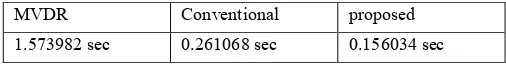
The performance of the proposed algorithm is compared with that of the conventional method using FFT and the high resolution MVDR method.. Figures 2 and 3 demonstrates the convergence of the estimated parameters at various SNRs[-10,-5,0,5] for true DOAs 0f 700 and 300. The initial values were assumed to be [ 580, 250] respectively. Figure 6 compares the convergence of the algorithm for a true DOA of 600 at an SNR of 5.The RMSE and CRB of the proposed method is compared against the RMSE of the conventional and MVDR methods in fig 7. Fig 8 illustrates the variation of RMSE with SNR, for all the three methods. The MVDR method exhibits zero variance. This may be due to the fact that, in the MVDR method, the DOA is obtained by plotting the energy against different angles and picking the point at which peak energy occurs.
Table 1 presents the mean and variance of the DOA estimation based on the three methods for various true values of DOA. The percentage estimation error for the proposed method falls in the range of -1.32 to 12.86, where as that for the conventional method is between -0.0958 to 7.78. The variance of the proposed method lie in the range of 0.0262 and 0.0543 where as the variance in the conventional method is in the range 0.000099 – 0.2377. The MVDR gives zero variance for all DOAs and SNRs as it is a high resolution method.
The execution time of the proposed algorithm is less than that of the conventional and MVDR methods and hence they are fast enough to be implemented in real time.
Table 1 lists the means and variances of the DOA estimates based on the three methods for various true values of DOA. Table
2 compare the time required for convergence of the three methods. The execution time for 100 simulations using a PC with an AMD Athlon 64 (2GHz clock frequency) processor was computed. The execution times for the proposed method and MVDR method are 0.156034 seconds 0.261068 seconds respectively. It is clear that the proposed method converges fast
.
5.
CONCLUSION
A model and an algorithm for the DOA estimation using EKF is discussed in this paper. The DOA problem has been reformulated in state space. We then propose the use of EKF for identifying the interpolation coefficients to produce the phase delayed signals at any sensor of uniform linear array using samples of the signals at the previous sensor. The results of the proposed algorithm are compared with the results obtained using conventional and MVDR methods. DOA as well as the interpolation coefficients of the second order model were treated as the augmented states of the EKF, thereby reducing the estimation to a system identification problem. The EKF brings out an algorithm that is suitable for recursive estimation of DOA.. The performance of the model and algorithm is compared with the popular MVDR and conventional methods. It has been found that the proposed method converges close to the true value and convergence time is less. In terms of variance of the estimates, the performance of the proposed method is better than that of the conventional method..
The problem addressed is an important one, both in theoretical and in practical applications in signal processing. The presented analysis is to highlight the ability of EKF to estimate DOA. Effort is made to treat DOA estimation as parameter estimation problem, using EKF. The flexibility in choosing the parameter set and fast convergence, suggest that the proposed algorithm is a useful tool for estimating DOA in the case of isolated targets. The foremost advantage of the algorithm, we propose is the simplicity, as computationally it is not very demanding. The problem reformulation allows for power techniques to be brought in for solving the DOA estimation problem.
Volume 1 – No. 1
22
0 100 200 300 400 500 600 700 800 900 20
25 30 35 40 45 50 55 60
Num ber of s napshots
E
s
ti
m
a
te
d
d
o
a
,d
e
g
[image:5.612.69.274.72.218.2]S NR 5 S NR 0 S NR -5 S NR -10
Fig.2 convergence of the proposed algorithm for true DOA = 30 deg.
0 100 200 300 400 500 600 700 800 900 58
60 62 64 66 68 70 72 74 76 78 80
Number of snapshots
E
s
ti
m
a
te
d
d
o
a
,d
e
g
[image:5.612.329.553.86.315.2]S NR 5 S NR 0 S NR -5 S NR -10
Fig.3 convergence of the proposed algorithm for true DOA = 70 deg.
0 10 20 30 40 50 60 70 80 90 100
1 1.5 2 2.5 3 3.5 4 4.5 5 5.5x 10
-4
No of iterations
v
a
ri
a
ti
o
n
o
f
p
a
ra
m
e
te
r
b
Fig.4 Convergence of the interpolation coefficient b
0 10 20 30 40 50 60 70 80 90 100
0.8 1 1.2 1.4 1.6 1.8 2
No of iterations
v
a
ri
a
ti
o
n
o
f
p
a
ra
m
e
te
r
a
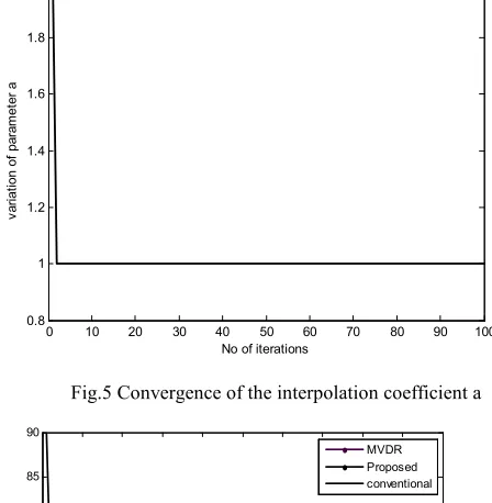
Fig.5 Convergence of the interpolation coefficient a
0 10 20 30 40 50 60 70 80 90 100
55 60 65 70 75 80 85 90
No of iterations
E
s
ti
m
a
te
d
D
O
A
[image:5.612.67.270.270.412.2]MVDR Proposed conventional
Fig.6 Comparison of the convergence of the three methods for true DOA = 60 deg.
0 100 200 300 400 500 600 700 800 900 1000 -0.1
0 0.1 0.2 0.3 0.4 0.5 0.6 0.7 0.8 0.9
Snapshots
R
M
S
E
,
d
e
g
crb proposed conventional MVDR
[image:5.612.67.288.466.647.2] [image:5.612.329.540.486.635.2]Volume 1 – No. 1
23
0 5 10 15 20 25
-0.01 0 0.01 0.02 0.03 0.04 0.05
SNR
R
M
S
E
[image:6.612.62.274.74.234.2]mvdr proposed conventional
[image:6.612.54.305.365.476.2]Fig.8 Variation of RMSE with SNR for true DOA =60 deg
Table 1 Mean and variances of estimation of the three algorithms (Method 1-conventional, Method II – MVDR, Method III – proposed)
Table 2.Comparison of execution times of the three methods
6. REFERENCES
[1] J. Li, P. Stoica, Zhisong Wang, “Doubly constrained Robust Capon Beamforme”, IEEE Trans. Signal Processing, Vol.52, 2004.
[2] P. J. Chung, J. F. Bohme, “Comparative Convergence Analysis of EM and SAGE Algorithms in DOA Estimation”, IEEE Trans. Signal Processing,2001.
[3] S. Haykin and A. Steinhardt, 1992 Adaptive Radar Detection and Estimation, John Wiley and Sons,.
[4] H. Cox, R.M. Seskind, and M.M. Owen, “Robust Adaptive Beamforming”, IEEE Trans. Acoustics, Speech and Signal Processing, Vol.35(10), 1987.
[5] J. Capon, “High-Resolution frequency –wave number spectrum analysis”, IEEE Trans. Signal processing , Vol.57, 1969. [6] P. Stoica, K.C. Sharman, “Maximum Likelihood Methods for Direction of Arrival Estimation”, IEEE Trans. Acoust.,Speech, Signal Processing, Vol. 38, July 1990.
[7] R. Roy, T. Kailath, “ESPRIT – Estimation of Signal Parameter via Rotational Invariance Techniques”, IEEE Trans. Signal Processing, Vol. 37, July 1989.
[8] M. Viberg , B. Otterson, T. Kailath, “Detection and Estimation in Sensor Arrays using Weighted Subspace Fitting”, IEEE Trans. Signal Processing, Vol.39, 1991.
[9] M. Viberg, B. Otterson, “Sensor Array Processing based on Subspace Fitting”, IEEE Trans. Signal Processing, Vol.39, May 1991.
[10] A. Farina, 1992 Antenna – Based Signal Processing Techniques for Radar Systems.,Artech House inc, Boston. [11] D. Kong and J. Chun,2000 A fast DOA Tracking Algorithm Based on the Extended Kalman filter. In Proceedingsof National Aerospace and Electronics Conference, NAECON 2000.
[12] E.F. Sagiroglu,1999 Localization of Wide-band Signals via Extended Kalman Filter. In Proceedings of IEEE International Symposium on Circuits and Systems( Vol.4, Jul 1999).
[13] R.A. Mucci, “A comparison of Efficient Beamforming Algorithms”, IEEE Trans. Acoust.,Speech and Signal Processing,Vol.32,June 1984,pp. 548-558.
[14] Y. Wu, H.C. So, P.C. Ching, “Joint Time Delay and Frequency Estimation via State Space Realization”, IEEE Signal Processing Letters,Vol. 10, Nov. 2003.
[15] R.D. Rao, “Sensitivity Consideration in a State Space Model Based Harmonic Retrievel Methods”, IEEE Trans. Acoust., Speech, Signal Processing, Vol. 37, 1989.
[16] C.K. Chui and Chen,1991 Kalman Filtering with Real – Time Applications, Springer Verlag, New York.
[17] T. Lefebvre, Herman Bruynincks,Joris De Schutter , “Online Statistical Model Recognition and State Estimation for Autonomous Compliant Motion”, IEEE Trans. Systems, Man, and Cybernetics, Part C, Vol. 35, 2005.
[18] R.G. Pridham and R.A.Mucci,1979 Digital Interpolation Beamforming for lowpass and Bandpass Signals.In proceedings IEEE (Vol.67,June 1979).
MEAN,VARIANCES AT SNR=5dB FOR DIFFERENT ANGLES OF ARRIVAL
DOA Method I Method II Method III MEAN VAR MEAN VAR MEAN VAR
15 14.1035 0.2187 15.00 0.0 16.9291 0.0485 30 32.3341 0.0524 30.00 0.0 29.0107 0.0543 45 45.4114 0.00016 45.00 0.0 44.0052 0.0322 60 59.749 0.2377 60.00 0.0 59.0055 0.0517 75 74.9281 0.000099 75.00 0.0 74.0035 0.0262
MVDR Conventional proposed
[image:6.612.47.300.521.553.2]Volume 1 – No. 1
24 [19] R. Togneri, Li Deng, “Joint State and Parameter Estimation
for a Target –Directed Non-linear Dynamic Model”, IEEE Trans. Signal Processing,Vol. 51, 2003.
[20] N. Kalouptsidis, Theoridis,1993 Adaptive System Identification and Signal Processing Algorithms , Prentice Hall, New York,1993.