A Feedback Neural Network for Solving Nonlinear
Programming Problems with Hybrid Constraints
Hamid Reza Vahabi
Department of Mathematics, Eslamshahr Branch,
Islamic Azad University, Tehran, Iran
Hasan Ghasabi-Oskoei
Department of Mathematics, Eslamshahr Branch,
Islamic Azad University, Tehran, Iran
ABSTRACT
This paper proposes a high-performance feedback neural network model for solving nonlinear convex programming problems with hybrid constraints in real time by means of the projection method. In contrary to the existing neural networks, this general model can operate not only on bound constraints, but also on hybrid constraints comprised of inequality and equality constraints. It is shown that the proposed neural network is stable in the sense of Lyapunov and can be globally convergent to an exact optimal solution of the original problem under some weaker conditions. Moreover, it has a simpler structure and a lower complexity. The advanced performance of the proposed neural network is demonstrated by simulation of several numerical examples.
General Terms
Neural Networks, Nonlinear Programming Problems.
Keywords
Nonlinear programming, Feedback neural network, Global convergence and stability.
1.
INTRODUCTION
In the recent years many artificial neural networks developed to solve the optimization problems, because it has many important applications in wide variety of scientific and engineering fields including network economics, transportation science, game theory, military scheduling, automatic control, signal processing, regression analysis, structure design, mechanical design, electrical networks planning, and so on [1]. In many scientific and engineering applications, it is desire to have real-time on-line solutions of optimization problems [2]. Traditional optimization algorithms [1, 3, 4, 5, 6 and 7] are not suitable for real-time on-line implementation on digital computers. One promising approach to handle these difficulties is to employ an artificial neural network based on circuit implementation. The most important advantages of the neural networks are massively parallel processing and fast convergence. Many continuous-time neural networks for constrained optimization problems have been developed using penalty parameters [8, 9 and 10]. To avoid the penalty parameters, some significant works have done in recent years [11, 12, 13, 14, 15 and 16].
In this paper, we propose a class of neural networks with one hidden layer structure in order to solve nonlinear convex programming problems with hybrid constraints in real time. This model ofneural networks has no adjustable parameters and therefore has lower complexity. The projection operator on a closed convex set is employed to describe the network to solvenonlinear programming problem. We define a suitable Liapunov function and prove the global convergence of the network.
The paper organized as follow. In the next section we introduce nonlinear programming problem with bound constraints and its equivalent formulation is described.In section 3, a feedback neural network model with circuit implementation is proposed. Section 4 discusses the stability of the proposed network and analyzes its global convergence. Extension of a proposed neural network for solving nonlinear programming problems with hybrid constraints is given in Section 5.In Section 6, numerical examples are simulated to show the reasonableness of our theory and demonstrate the high performance of proposed neural networks approach. A comparative analysis is presented in Section 7. Some conclusions are summarized in the last section.
2.
NONLINEAR PROBLEM WITH BOUND
CONSTRAINTS AND FORMULATION
Consider the following nonlinear convex programming problem with bound constraints:min
( )
. .
,
f x
s t
A x
b
l
x
h
≤
≤ ≤
(1)
where
f
:
n→
is nonlinear, convex and twice continuously differentiable,b
∈
m,A
ism
×
n
matrix and, ,
nx l h
∈
.Lemma 1. Suppose
Χ
is a closed convex set, for anyk
z
∈
, there is a unique pointP z
Χ( )
∈ Χ
such that( )
inf
u
z
P z
Χz
u
∈Χ
−
=
−
( )
P z
Χ is called the projection ofz
onΧ
andP
Χis called the projection operator onΧ
. Moreover,,
k:
( )
( )
u z
P z
ΧP u
Χz
u
∀
∈
−
≤
−
For
u
∈
k,
u
∈ Χ
, (
u
−
u
) (
Tu
−
z
)
≥
0
for allz
∈ Χ
if and only if
u
=
P u
Χ( )
.Proof. See [17 and 18].
We first give a sufficient and necessary condition for the solution of problem (1). It is the theoretical foundation for us to design the network for optimization problems.
Suppose that
Χ =
0{
y
=
(
y
1,
,
y
m)
T∈
m}
, 0( )
(
0(
1),
,
0(
))
T m
P
Χy
=
P
Χy
P
Χy
and for
i
=
1,
,
m
;0
(
i)
max{0,
i}
Fig. 1: Block diagram of the feedback neural network (3).
1
{
x
(
x
,
,
x
n)
T nl
x
h
}
Χ =
=
∈
≤ ≤
,1
( )
(
(
),
,
(
n))
TP x
Χ=
P x
Χ
P x
Χ and forj
=
1,
,
n
(
)
j j j
j j j j j
j j j
l
x
l
P x
x
l
x
h
h
x
h
Χ
<
=
≤
≤
>
According to the Karush-Kuhn-Tucker condition [19] and using the projection theorem [20], we can obtain easily the following lemma.
Lemma 2.
x
*is an optimal solution of (1) if and only if thereexists
y
*∈
m, such that(
x
*,
y
*)
T satisfies the following equations0
(
( )
)
0
(
)
0
T
x
P x
f x
A y
y
P
y
A x
b
Χ Χ
−
− ∇
−
=
−
+
−
=
(2)Proof. See [20].
3.
NEURAL NETWORK MODEL AND
CIRCUIT IMPLEMENTATION
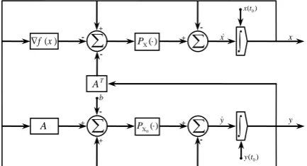
Based on the equivalent formulation in Lemma 2, we propose a feedback neural network for solving (1), with its time dependent dynamical system being given by
0
0 0
0 0
(
( )
)
(
)
( )
,
( )
T
dx
P x
f x
A y
x
dt
dy
P
y
A x
b
y
dt
x t
x
y t
y
Χ
Χ
=
− ∇
−
−
=
+
−
−
=
=
(3)
where
x
∈
n,y
∈
m. AlsoP
Χ( )
⋅
and0
( )
P
Χ⋅
are projection operators onΧ
andΧ
0. We shall prove that network (3) is globally convergent to the solutions set of problem (1). The dynamical equations described by (3), can be easily realized by a feedback neural network with a single-layer structure as shown in Fig. 1. Where the vectorsx t
( )
0 andy t
( )
0 are the initial external inputs andx
andy
are the network outputs.4.
STABILITY AND CONVERGENCE OF
THE NETWORK
In this section, we shall study the dynamics of network (3). We first define a suitable Liapunov function and then prove the global convergence of network (3) in Theorem 2.
Theorem 1. For any
x t
( )
0∈ Χ
andy t
( )
0∈ Χ
0, the neuralnetwork (3) has a unique solution
z t
( )
=
( ( ), ( ))
x t
y t
T .Proof. Let
0
(
( )
)
( )
(
)
T
P x
f x
A y
x
M z
P
y
A x
b
y
Χ
Χ
− ∇
−
−
=
+
−
−
By lemma 1, note that
P x
Χ(
− ∇
f x
( )
−
A y
T)
and0
(
)
P
Χy
+
A x
−
b
are Lipschitz continuous. Then it is easy tosee that
M z
( )
is also Lipschitz continuous. From the existence and uniqueness theorem of ordinary differential equations [21], there exists a unique solutionz
(
t
)
with0 0 0
( )
( ( ), ( ))
Tz t
=
x t
y t
for the neural network (3).Theorem 2. Let
2 0
1
( ) ( ( ( ))) ( ) ( ( )) 2
T
E z = z −P zΧ −F z F z − P zΧ −F z −z and
( )
( )
,
T
f x
A y
F z
b
A x
∇
+
=
−
then
E z t
( ( ))
that is defined as follow is Liapunov function of system (3).2 * 0
1
( ( ))
( )
( )
2
E z t
=
E z
+
z t
−
z
Where
z
* is an equilibrium point of (3). Moreover, the network (3) is globally convergent to the solutions set of problem (1).Proof. We have
0
( )
( )
( )(
(
( ))
)
(
( ))
dE z
F z
F z
P z
F z
z
du
P z
F z
z
Χ
Χ
=
− ∇
−
−
+
−
−
Let
g z
( )
=
P z
Χ(
−
F z
( ))
−
z
, then(
*)
( )
( )
( )
( ) ( )
( )
( )
T
T
dE z
dE z
dz
dt
dz
dt
F z
F z g z
g z
z
z
g z
=
=
− ∇
+
+ −
(
*)
2( )
T( )
( )
( )
T( ) ( )
F z
z
z
g z
g z
g z
F z g z
=
+ −
+
−
∇
In the inequality of Lemma 1, let
u
= −
z
F z
( )
and let*
x
=
z
, we get*
( ( )
g z
+ −
z
z
) (
T−
g z
( )
−
F z
( ))
≥
0
Then2
* *
( ( )
F z
+ −
z
z
)
Tg z
( )
≤ −
F z
( ) (
Tz
−
z
)
−
g z
( )
( )
f x
∇
∑
PΧ( )⋅∫
T
A
0
( ) x t
0
( )
y t
y
∑
0( )
PΧ ⋅
x
y x
∑
∑
A
+
+
+
+ +
-b
∫
-It follows that
2 *
2
*
( )
( ) (
)
( )
( )
( )
( ) ( )
( ) (
)
( )
( ) ( )
0
T
T
T T
dE z
F z
z
z
g z
dt
g z
g z
F z g z
F z
z
z
g z
F z g z
≤ −
−
−
+
−
∇
= −
−
−
∇
≤
On the other side, in the inequality of Lemma 1, let
( )
u
= −
z
F z
and letx
=
z
, we obtain2
( )
T( )
( )
F z
g z
≤ −
g z
It follows that 0
( )
1
( )
22
E z
≥
g z
and thus(
2 * 2)
* 21
1
( )
( )
2
2
E z
≥
g z
+
z
−
z
≥
z
−
z
.Since
E z
( )
is positive definite and radially unbounded, for any initial pointz t
( )
0 there exists a convergent subsequence{
z t
( )
k}
such thatlim ( )
kˆ
k→∞
z t
=
z
, whereˆ
( )
0
dE z
dt
=
. Wenext prove that
dE z
( )
ˆ
0
dt
=
if and only ifz
ˆ
is a KKT point.Note that
∇
F z
( )
is positive semi-define and*
( ) (
T)
0
F z
z
−
z
≥
. Then*
( )
( ) (
T)
( )
T( ) ( )
0
dE z
F z
z
z
g z
F z g z
dt
≤ −
−
−
∇
≤
.Moreover,
dE z
( )
ˆ
0
dt
=
if and only if(
)
(
)
*
ˆ
ˆ
( ) (
)
0
ˆ
ˆ
ˆ
ˆ
ˆ
ˆ
ˆ
(
( ))
( )
(
( ))
0
T
T
F z
z
z
P z
ΧF z
z
F z
P z
ΧF z
z
−
=
−
−
∇
−
−
=
It can be seen that
(
)
(
)
(
)
2(
)
ˆ ˆ ˆ ˆ ˆ ˆ ˆ
( ( )) ( ) ( ( ))
ˆ ˆ ˆ ˆ ˆ ˆ ˆ ˆ ˆ
( ( ) ) ( ) ( ( ) )
T
T
T T
P z F z z F z P z F z z
P x f x A y x f x P x f x A y x
Χ Χ
Χ Χ
− − ∇ − −
= − ∇ − − ∇ − ∇ − −
where
z
ˆ
=
( , )
x y
ˆ ˆ
T , and∇
2f x
( )
ˆ
is Hessian matrix. Since∇
2f x
( )
is positive definite(
P x
Χ(
ˆ
− ∇
f x
( )
ˆ
−
A y
Tˆ
)
−
x
ˆ
)
=
0
thusˆ
ˆ
ˆ
0 :
(
) (
T( )
T)
0
x
x
x
f x
A y
∀ ≥
−
∇
+
≥
using
*
* * *
ˆ
ˆ
ˆ
(
) (
( )
)
0
ˆ
(
) (
(
)
)
0
T T
T T
x
x
f x
A y
x
x
f x
A y
−
∇
+
≥
−
∇
+
≥
we get
(
)
* * *
ˆ
ˆ
ˆ
(
x
−
x
)
T∇
f x
(
)
+
A y
T− ∇
(
f x
( )
+
A y
T)
≥
0
thus
(
)
(
)
* *
* * * *
ˆ
ˆ
(
)
ˆ
ˆ
(
)
(
)
( )
) .
T T T
T T T
x
x
A y
A y
x
x
f x
A y
f x
A y
−
−
≥
−
∇
+
− ∇
−
On the other side,
P x
Χ( )
is monotone. That is, for anyx
andy
(
P x
Χ( )
−
P
Χ( )
y
)
T(
x
−
y
)
≥
0
then*
* * *
ˆ
ˆ
ˆ
ˆ
(
) (
(
( )
)
(
(
(
)
)))
0
T T
T
x
x
x
f x
A y
x
f x
A y
−
− ∇
+
−
− ∇
+
≥
It follows that
(
)
2
* * *
* * * *
ˆ
(
ˆ
) (
ˆ
)
ˆ
ˆ
2(
)
( )
(
(
)
)
T T T
T T T
x
x
x
x
A y
A y
x
x
f x
A y
f x
A y
−
≥
−
−
≥
−
∇
+
− ∇
+
let
(
)
* * * *
ˆ
ˆ
(
x
x
)
Tf x
( )
A y
T(
f x
(
)
A y
T)
γ
=
−
∇
+
− ∇
+
If
x
ˆ
≠
x
*, thenγ
>
0
, since∇
f x
( )
+
A y
T *is strictly monotone. It follows that when
γ
=
x
ˆ
−
x
* 2 then2 2 2
* * *
ˆ
2
ˆ
ˆ
x
−
x
≥
x
−
x
>
x
−
x
.This would constitute a contradiction. So
x
ˆ
=
x
*andˆ
0
A x
− ≤
b
.Now,
F z
( ) (
ˆ
Tz
ˆ
−
z
*)
=
0
implies that
* *
ˆ
ˆ
ˆ
ˆ
ˆ
(
x
−
x
) (
T∇
f x
( )
+
A y
T)
−
(
y
−
y
) (
TA x
−
b
)
=
0 .
Sincex
ˆ
=
x
*,(
y
ˆ
−
y
*) (
TA x
ˆ
−
b
)
=
0
. Thus
* * *
ˆ
ˆ
ˆ
( ) (
y
TA x
−
b
)
=
(
y
) (
TA x
−
b
)
=
(
y
) (
TA x
−
b
)
=
0
Therefore,z
ˆ
=
( , )
x y
ˆ ˆ
Tis a KKT point. Finally, define again
2 0
1
ˆ
( ( ))
( ( ))
( )
ˆ
2
E z t
=
E z t
+
z t
−
z
Then,
E z
ˆ ˆ
( )
=
0
and thuslim
ˆ
( ( ))
kˆ ˆ
( )
0
k→∞
E z t
=
E z
=
.So, for
∀ >
ε
0
there existsη
>
0
such that for allt
k≥
t
ηwe have
E z t
ˆ
( ( ), )
kz
ˆ
<
ε
.Similar to the previous analysis, we have
d
E z t
ˆ ( ( )) 0
dt
≤
.So, for
t
≥
t
ηˆ
ˆ
ˆ
( )
2 ( ( ))
( ( ))
2
z t
−
z
≤
E z t
≤
E z t
η≤
ε
.It follows that
lim
( )
ˆ
0
5.
NEURAL NETWORK FOR NONLINEAR
PROBLEM WITH HYBRID CONSTRAINTS
Corollary 1. Suppose nonlinear programming problem is as follows
1 1
2 2
min
( )
. .
f x
s t
A x
b
A x
b
l
x
h
≤
=
≤ ≤
(4)
If
y
andw
are dual variables vectors of inequality and equality constraints, then the neural network (3) changes into the following form:0
1 2
1 1
2 2
0 0 0
0 0 0
(
( )
)
(
)
( )
,
( )
,
( )
T T
dx
P x
f x
A y
A w
x
dt
dy
P
y
A x
b
y
dt
dw
b
A x
dt
x t
x
y t
y
w t
w
Χ
Χ
=
− ∇
−
+
−
=
+
−
−
=
−
=
=
=
(5)
Corollary 2. We can have same analytical discussions about
neural network (5) and handle them to reach optimum solution of problem (4).
6.
SIMULATION EXAMPLES
We discuss the simulation results using numerical examples to demonstrate the global convergence property and effectiveness of the proposed neural networks. We have written a Matlab 2010 code for solving models (3) and (5) and executed the code on an Intel Corei5. Based on numerical simulations, the proposed models have a very fast convergence to exact optimal solutions of problems (1) and (4). This is one of the advantages of our networks in comparison with existing neural networks.
Example 1. Consider the following nonlinear programming
problem:
4 2 4 2
1 1 2 2 1 2
1 2
1 2
1 2
1 2
1
1
1
1
min
0.9
4
2
4
2
2
2
. .
3
2
,
0
x
x
x
x
x x
x
x
x
x
s t
x
x
x x
+
+
+
−
+
≤
− + ≤
−
≤ −
≥
(6)
This problem has an optimal solution *
(0.427, 0.809)T
x = . It
can be seen that objective function is strictly convex and the feasible region is a convex set. Note that
3
1 1 2
3
2 2 1
0.9
( )
0.9
x
x
x
f x
x
x
x
+
−
∇
=
+
−
and
-3 -2 -1 0 1 2 3
-3 -2 -1 0 1 2 3
x1
x
[image:4.610.325.554.75.263.2]2
Fig.2: Transient behavior
(
x x
1,
2)
T of proposed neuralnetwork (3) with various initial points in Example 1.
2
2 1
2 2
3
1
0.9
( )
0.9
3
1
x
f x
x
+
−
∇
=
−
+
is positive–definite on
Χ
. Theorem 2 guarantees that the neural network (3) is globally convergent to optimal solution of problem (6). We use the neural network (3) to solve this problem. Simulation results show the trajectories of (3) with any initial points are always convergent tox
*. The feasible region and the transient behavior(
x x
1,
2)
T based on (3) with various initial points are displayed in Fig. 2. Starting points for dual variables are random.Example 2. Consider the following nonlinear programming
problem:
2 2 2 2
1 2 3 4 1 4
1 2 3 4 1 4
1 2
3 4
1 2
3 4
3
min
(
)
2(
)
ln(
)
2
3
4
2
3
1
1
. .
0.1
10,
0
10,
0
10, 0.1
10
x
x
x
x
x x
x x
x x
x
x
x
x
x
x
s t
x
x
x
x
+
+
+
−
+
+
−
−
+
=
+ =
≤
≤
≤
≤
≤
≤
≤
≤
(7)
The nonlinear programming problem (7) has the exact optimum solution
x
*=
(1, 0, 0,1)
T while its dual has the optimum solution*
(0, 0)
Ty
=
. The model (5) is used to find optimal solutions*
x
andy
*, simultaneously. The convergent path for the variables1 2 3 4 1 2
( , )
x y
T=
(
x x
,
,
x
,
x
,
y y
)
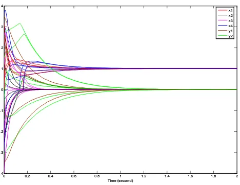
T is shown in Fig. 3 with various random starting points. Simulation results show that the neural network (5) is globally convergent tox
*andy
*. The obtained solutions are absolutely exact and real time.*
(0.427, 0.809)T
0 0.2 0.4 0.6 0.8 1 1.2 1.4 1.6 1.8 2 -4
-3 -2 -1 0 1 2 3 4
Time (second)
[image:5.610.57.291.74.255.2]x1 x2 x3 x4 y1 y2
Fig. 3. The trajectories of proposed neural network (5) with
various random starting points in Example 2
.
Example 3. Consider the following nonlinear programming
problem:
2 2 2 2 3
1 1 2 1 2 3 4 1
1 2 3
1 2 3 4
1 2 4
1 2 3 4
1
min 0.4
0.5
0.5
30
2,
3
18,
. .
1
2,
3
,
,
,
0
x
x
x
x x
x
x
x
x
x
x
x
x
x
x
s t
x
x
x
x x x x
+
+
−
+
+
+
− +
−
≤
+
−
−
≤
+
−
=
≥
(8)
This problem has an optimal solution
x
*=
(0.982,1.672,0,0) .
TFig. 4 show that all state variable trajectories of neural network (5) are globally convergent to the optimal solution
* * * *
( , , )T (0.982,1.672, 0, 0, 0, 0, 2.363)T
z = x y w = in problem
(8) and its dual, simultaneously. These trajectories indicate fast convergence to exact optimal solutions.
7.
COMPARATIVE ANALYSIS
To see how well the present neural network model is, we compare it with one existing network model for solving nonlinear convex programming problems. Consider (4) is
min
( )
. .
f x
s t
A x
b
l
x
h
=
≤ ≤
(9) Then the neural network (5) is as follows
(
( )
T)
dx
P x
f x
A y
x
dt
dy
b
A x
dt
Χ
=
− ∇
+
−
= −
(10)
Neural network model for solving (9) was developed in [15]. Its dynamical equation is described by
0 0.1 0.2 0.3 0.4 0.5 0.6 0.7 0.8 0.9 1 -4
-3 -2 -1 0 1 2 3 4 5
Time (second)
x1 x2 x3 x4 y1 y2 w1
Fig. 4. The trajectories of proposed neural network (5) with various arbitrary initial points in Example 3.
(
( )
)
(
( )
)
T
T
dx
P x
f x
A y
x
dt
dy
A P x
f x
A y
b
dt
ΧΧ
=
− ∇
+
−
= −
− ∇
+
+
(11)
It has two layers and because of an additional nonlinear term, it is more complex in structure than the proposed neural network model (10).
Therefore our network implementation is more
economical, which is very important for implementing of
the large-scale neural network.
8.
CONCLUDING REMARKS
We have proposed a feedback neural network for solving nonlinear convex programming problems with hybrid constraints in real time using the projection technique. We have also given a complete proof of the stability and global convergence of the proposed network by definition of a suitable Liapunov function. Compared with the existing neural network for solving such problems, the proposed neural network has a simple single layer structure, without a penalty parameter and amenable to parallel implementation. The simulation results displayed the reasonableness of our theory and fast convergence of the proposed neural networks to exact optimal solutions of nonlinear optimization problems.
9.
ACKNOWLEDGMENTS
The authors gratefully acknowledge the financial and other support of this research, provided by Islamic Azad University, Eslamshahr Branch, Tehran, Iran. Also the authors would like to thank M. Saderi-Oskoei for her valuable comments and discussions.
10.
REFERENCES
[1] Bazaraa, M.S., Sherali, H.D., and Shetty, C.M. 1993. Nonlinear Programming Theory and Algorithms, 2nd ed. New York: Wiley.
[image:5.610.324.558.74.254.2][3] Avriel, M. 1976. Nonlinear Programming: Analysis and Methods. Englewood Cliffs, NJ: Prentice-Hall.
[4] Fletcher, R. 1981. Practical Methods of Optimization. New York: Wiley.
[5] Harker, P.T. and Pang, J.S. 1990. Finite-dimensional variational inequality and nonlinear complementarity problems: A survey of theory, algorithms, and applications, Mathematical Programming, 48, 161–220.
[6] He, B.S. and Liao, L.Z. 2002. Improvements of some projection methods for monotone nonlinear variational inequalities, Journal of Optimization Theory and Applications 112(1), 111–128.
[7] He, B.S. and Zhou, J. 2000. A modified alternating direction method for convex minimization problems, Applied Mathematics Letters 13(2), 123–130.
[8] Kennedy, M.P. and Chua, L.O. 1988. Neural networks for nonlinear programming, IEEE Transactions on Circuits and Systems 35(5), 554–562.
[9] Lillo, W.E., Loh, M.H., Hui, S. and Zak, S.H. 1993. On solving constrained optimization problems with neural networks: A penalty method approach, IEEE Transactions on Neural Networks 4(6), 931–940.
[10]Rodríguez-Vázquez, A., Domínguez-Castro, R., Rueda, A., Huertas, J.L. and Sánchez-Sinencio, E. 1990. Nonlinear switched-capacitor ‘neural networks’ for optimization problems, IEEE Transactions on Circuits and Systems 37(3), 384–397.
[11]Ghasabi-Oskoei, H. 2005. Numerical solutions for constrained quadratic problems using high-performance neural networks, Applied Mathematics and Computation 169(1), 451–471. [12]Ghasabi-Oskoei, H. and Mahdavi-Amiri, N. 2006. An
efficient simplified neural network for solving linear and quadratic programming problems, Applied Mathematics and Computation 175(1), 452–464.
[13]Ghasabi-Oskoei H. 2007. Novel artificial neural network with simulation aspects for solving linear and quadratic programming problems, Computers and Mathematics with Applications 53, 1439–1454.
[14]Leung, Y., Chen, K. and Gao, X. 2003. A high-performance feedback neural network for solving convex nonlinear programming problems, IEEE Transactions on Neural Networks 14(6), 1469–1477.
[15]Tao, Q., Cao, J.D., Xue, M.S. and Qiao, H. 2001. A high performance neural network for solving nonlinear programming problems with hybrid constraints, Phys. Lett. A, 288(2), 88–94.
[16]Xia, Y.S. 1996. A new neural network for solving linear and quadratic programming problems, IEEE Transactions on Neural Networks 7(6), 1544–1547.
[17]Kinderlerer, D. and Stampcchia, G. 1980. An Introduction to Variational Inequalities and Their Applications, Academic Press, New York.
[18]Zhang, X., Li, X. and Chen, Z. 1982. The Theory of Ordinary Differential Equations in Optimal Control Theory, Advanced Educational Press, Beijing, in Chinese. [19]Luenberger, D.G. 1989. Introduction to Linear and
Nonlinear Programming, Addison-Wesley Reading, MA, Chapter 12.
[20]Bertsekas D.P. and Tsitsiklis, J. N. 1989. Parallel and Distributed Computation: Numerical Methods. Englewood Cliffs, NJ: Prentice-Hall.