Estimation in Misclassified Size Biased Generalized Negative Binomial Distribution

(1)

Estimation in Misclassified Size-Biased Generalized

Negative Binomial Distribution

B. S. Trivedi

1,*

_,

_{M. N. Patel}

2

1_{H. L. Institute of Commerce, Ahmedabad University, Navrangpura, Ahmedabad} 2_{Department of Statistics, School of Sciences, Gujarat University, Ahmedabad}

Corresponding Author: [email protected]

Abstract

In this paper, we are concerned with the situations, where sometimes value two is reported erroneously as one in

relation to size biased generalized negative binomial distribution (SBGNBD) with probability𝛼𝛼. We have obtained the Maximum likelihood estimator and Bayes estimator under general entropy loss function. A simulated study is carried out to access the performance of the maximum likelihood estimators and Bayes estimators. Also comparison has been made between maximum likelihood estimator and Bayes estimator.

Keywords

Misclassification, maximum likelihood estimator, Bayes estimator, general entropy loss function, simulation

1. Introduction

Pascal defined the negative binomial distribution as

𝑃𝑃[𝑋𝑋=𝑥𝑥] =�𝑚𝑚+_𝑥𝑥𝑥𝑥 −1� 𝜃𝜃𝑥𝑥₍₁_{− 𝜃𝜃}₎𝑚𝑚_(1.1)

𝑥𝑥= 0, 1, 2, … ….Where 0 <𝜃𝜃< 1 , 𝑚𝑚> 0

The mean and variance of the distribution are given as

𝐸𝐸(𝑋𝑋) = 𝜇𝜇1′ =₁𝑚𝑚𝜃𝜃_−𝜃𝜃 𝑎𝑎𝑎𝑎𝑎𝑎 𝑉𝑉(𝑋𝑋) =𝜇𝜇2=₍₁𝑚𝑚𝜃𝜃_−𝜃𝜃₎2 (1.2)

It can be easily seen that variance is always greater than mean.

This type of model was used to represent ‘accident-proneness’ by Greenwood and Yule

(1920). Wise (1946) describes an application of this kind of model to represent the distribution of number of pinholes per ‘unit’ length of enameled wire. The negative binomial distribution is very often a first choice as alternative when it is felt that a Poisson distribution might be inadequate.

A generalization of the negative binomial distribution so called generalized negative binomial distribution (GNBD) defined by Jain & Consul (1971) is given by

𝑃𝑃[𝑋𝑋=𝑥𝑥] =𝑝𝑝(𝑥𝑥;𝛼𝛼,𝜃𝜃) =_𝑚𝑚₊𝑚𝑚_{𝛽𝛽𝑥𝑥}�𝑚𝑚+_𝑥𝑥𝛽𝛽𝑥𝑥� 𝜃𝜃𝑥𝑥₍₁_{− 𝜃𝜃}₎𝑚𝑚+𝛽𝛽𝑥𝑥 −𝑦𝑦𝑥𝑥

=𝑚𝑚Γ(𝑚𝑚_𝑥𝑥+_!_Γ𝛽𝛽𝑥𝑥₍_𝑚𝑚) ₊𝜃𝜃𝑥𝑥_{𝛽𝛽𝑥𝑥 −𝑥𝑥}(1−𝜃𝜃₊₁₎)𝑚𝑚+𝛽𝛽𝑥𝑥 −𝑥𝑥 (1.3) with 0 <𝜃𝜃 < 1, 0≤ 𝛼𝛼 ≤1, 𝑚𝑚> 0 & |𝛽𝛽𝜃𝜃| < 1, 𝑥𝑥 ∈ 𝑇𝑇= {0, 1, 2, 3, … … … … }.

When the sampling mechanism selects units with probability proportional to some measure of the unit size, the resulting distribution is called size – biased. Such distributions arise in the life length and were studied by various authors. (see Gupta (1979, 1984), Gupta &. Tripathi (1987,1992), Williford and Binghan(1979)).

A size – biased GNBD is obtained by taking the weight of (1.3) as 𝑥𝑥, given by

𝑃𝑃[𝑋𝑋=𝑥𝑥] =𝑥𝑥. _𝐸𝐸𝑃𝑃₍_𝑥𝑥(₎𝑥𝑥)

(2)

𝑃𝑃(𝑋𝑋=𝑥𝑥) =𝑃𝑃[𝑥𝑥; 𝛼𝛼,𝜃𝜃] = 𝑚𝑚Γ(𝑚𝑚_𝑥𝑥_!_Γ+₍𝛽𝛽𝑥𝑥_𝑚𝑚₊)𝜃𝜃_{𝛽𝛽𝑥𝑥 − 𝑥𝑥}𝑥𝑥(1− 𝜃𝜃_{+ 1)})𝑚𝑚+𝛽𝛽𝑥𝑥 −𝑥𝑥× _{𝑚𝑚𝜃𝜃}𝑥𝑥

1− 𝜃𝜃𝛽𝛽

= Γ(𝑚𝑚+𝛽𝛽𝑥𝑥₍_𝑥𝑥−)𝜃𝜃𝑥𝑥−_1)!1_Γ(1₍−𝜃𝜃_𝑚𝑚₊)_{𝛽𝛽𝑥𝑥 −𝑥𝑥}𝑚𝑚+𝛽𝛽𝑥𝑥 −𝑥𝑥₊₁₎(1−𝜃𝜃𝛽𝛽 )

(1.4)

𝑥𝑥 ∈ 𝑇𝑇= {1, 2, 3, … … … … }

In experiments reported to discrete distributions, situations may often arise where the probabilities of different counts are affected in various ways. There may arise a situation where certain count is reported as some other count. e.g. when defective item is inspected wrongly as non defective item and vice versa. Cohen (1960) discussed this kind of situation where the count one is reported as count zero in case of Poisson and Binomially distributed random variables, whereas Jani and Shah (1979) studied the problem of misclassification in a class of discrete distribution, the power series distribution defined by Noack (1950) in which some of observations corresponding to the cell one are sometimes wrongly reported as observations corresponding to cell zero.

The problem of misclassification for the most general class of discrete distribution, misclassified generalized negative binomial distribution is considered by Gupta and Tripathi (1987) in some particular case of modified power series distribution and recently by Patel & Patel (1996, 2001) in the case of generalized power series distribution and modified power series distribution for a more general situation where sometimes the value (𝑐𝑐+ 1) is reported as 𝑐𝑐.

If we assume that some of the observations corresponding to the cell 𝑥𝑥= 2 are wrongly reported as belonging to the cell 𝑥𝑥= 1, and let this probability of misclassification be α. Then the probability function of the reported number of observations can be written as

𝑃𝑃[𝑋𝑋=𝑥𝑥] =� 𝑃𝑃𝑃𝑃((𝑥𝑥𝑥𝑥= 1) += 2)− 𝛼𝛼𝛼𝛼𝑃𝑃𝑃𝑃((𝑥𝑥𝑥𝑥= 2), = 2), 𝑓𝑓𝑓𝑓𝑓𝑓𝑓𝑓𝑓𝑓𝑓𝑓 𝑥𝑥𝑥𝑥= 2= 1

𝑃𝑃(𝑥𝑥), 𝑓𝑓𝑓𝑓𝑓𝑓 𝑥𝑥= 3, 4, 5, …

(1.5)

Suppose X is a random variable having the size – biased generalized negative binomial distribution (1.4) from which a random sample is drawn. Then the resulting distribution of X based on (1.5) is called misclassified size-biased generalized negative binomial distribution (MSBGNBD), which can be written in the form

𝑃𝑃[𝑋𝑋=𝑥𝑥] =𝑝𝑝(𝑥𝑥; 𝛼𝛼,𝜃𝜃) =

⎩ ⎨

⎧(1− 𝜃𝜃)𝑚𝑚+𝛽𝛽−1 (1− 𝜃𝜃𝛽𝛽) (1 +𝛼𝛼 (𝑚𝑚+ 2𝛽𝛽 −1)𝜃𝜃(1− 𝜃𝜃)𝛽𝛽−1 ,𝑥𝑥= 1

(1− 𝛼𝛼)(𝑚𝑚+ 2𝛽𝛽 −1)(1− 𝜃𝜃𝛽𝛽)𝜃𝜃(1− 𝜃𝜃)𝑚𝑚+2(𝛽𝛽−1)_,_𝑥𝑥_{= 2}

Γ(𝑚𝑚+𝛽𝛽𝑥𝑥) 𝜃𝜃𝑥𝑥−1₍₁_−𝜃𝜃₎𝑚𝑚+𝛽𝛽𝑥𝑥 −𝑥𝑥₍₁_{−𝜃𝜃𝛽𝛽}₎

(𝑥𝑥−1)! Γ(𝑚𝑚+𝛽𝛽𝑥𝑥 −𝑥𝑥+1) ,𝑥𝑥= 3, 4, . .∞ 𝑖𝑖.𝑒𝑒.𝑥𝑥 ∈ 𝑠𝑠

(1.6)

where 𝑠𝑠=𝑇𝑇 −{1, 2}

0≤ 𝛼𝛼 ≤1, 0 <𝜃𝜃< 1, 𝑚𝑚> 0 , |𝛽𝛽𝜃𝜃| < 1.

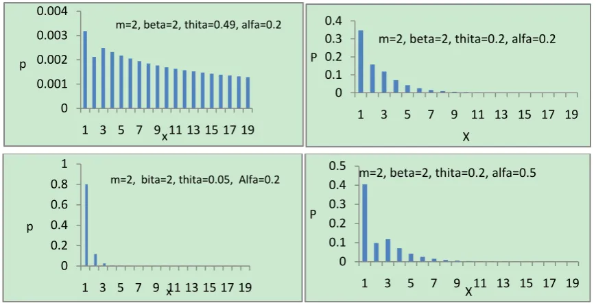
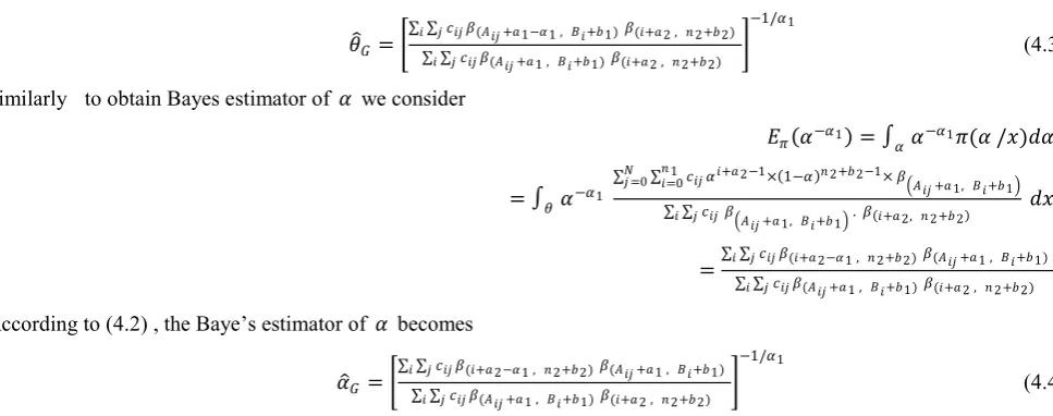
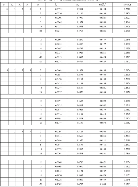
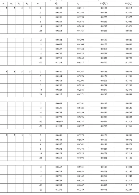
[image:2.595.88.523.525.746.2]

Under the different choice of the parameters of MSBGNBD, the graphs of the probability distribution are given below.

Figure 1. Plots of the p.m.f. of the misclassified size-biased generalized negative binomial distribution.

0 0.001 0.002 0.003 0.004

1 3 5 7 9 11 13 15 17 19 p

x

m=2, beta=2, thita=0.49, alfa=0.2

0 0.1 0.2 0.3 0.4

1 3 5 7 9 11 13 15 17 19 P

X

m=2, beta=2, thita=0.2, alfa=0.2

0 0.2 0.4 0.6 0.8 1

1 3 5 7 9 11 13 15 17 19 p

x

m=2, bita=2, thita=0.05, Alfa=0.2

0 0.1 0.2 0.3 0.4 0.5

1 3 5 7 9 11 13 15 17 19 P

X

(3)

This distribution is considered by Hassan and Ahmad (2009). Moments and some recurrence relations of the moments are derived.

In this paper we have considered the Maximum likelihood (ML) estimation and Bayes estimation of the parameters of MSBGNBD. In section 2 we have obtained ML estimators of the parameters and studied their properties by theorem. Section 3 describes Prior, Posterior and Marginal distribution of the parameters 𝜃𝜃 and 𝛼𝛼. In section 4, we have derived Bayes estimators under General entropy loss function (GELF). Comparison among different estimation methods using simulation study is presented in section 6.

2. Maximum Likelihood Estimators

Let 1, 2, 3, … … … . .𝑘𝑘 (where 𝑘𝑘 ∈{1, 2, … … .∞}) be the possible values of a random variable 𝑥𝑥 in a random sample of size N taken from the distribution given in (1.6). Let 𝛼𝛼 be the proportion of misreported number of observations corresponding to the cell 𝑥𝑥= 2 by reporting them as belonging to the cell 𝑥𝑥= 1.

Let 𝑎𝑎𝑘𝑘 denote the number of observations corresponding to the value 𝑥𝑥𝑘𝑘 in the sample, then we have

� 𝑎𝑎𝑖𝑖 =𝑁𝑁

𝑘𝑘

𝑖𝑖=1

The likelihood function 𝐿𝐿 of such a sample is given by

𝐿𝐿=� 𝑝𝑝𝑖𝑖𝑎𝑎𝑖𝑖 𝑘𝑘

𝑖𝑖=1

where 𝑝𝑝𝑖𝑖 =𝑝𝑝(𝑥𝑥=𝑖𝑖) ,𝑖𝑖= 1, 2, 3, … … … … .𝑘𝑘

𝐿𝐿=�𝜃𝜃(1− 𝜃𝜃)

𝛽𝛽−1_�𝑚𝑚₊_{𝛼𝛼𝑚𝑚}₍_𝑚𝑚_{+ 2}_{𝛽𝛽 −}₁₎_�𝜃𝜃₍₁_{− 𝜃𝜃}₎𝛽𝛽−1 _��

(1− 𝜃𝜃)−𝑚𝑚_._{� 𝑚𝑚𝜃𝜃}

1− 𝜃𝜃𝛽𝛽�

�

𝑎𝑎1

×

�(1−𝛼𝛼)𝑚𝑚 (𝑚𝑚+2𝛽𝛽−1)

(1−𝜃𝜃)−𝑚𝑚_._�𝑚𝑚𝜃𝜃

1−𝜃𝜃𝛽𝛽�

�𝜃𝜃 (1− 𝜃𝜃)𝛽𝛽−1 _�2_�𝑎𝑎2_×

∏ �₍_𝑖𝑖−_1)!𝑚𝑚_ΓΓ₍(_𝑚𝑚𝑚𝑚₊+_{𝛽𝛽𝑖𝑖 −𝑖𝑖}𝛽𝛽𝑖𝑖)₊₁₎ �𝜃𝜃 (1−𝜃𝜃)𝛽𝛽−1 �𝑖𝑖

(1−𝜃𝜃)−𝑚𝑚_._�𝑚𝑚𝜃𝜃

1−𝜃𝜃𝛽𝛽�

�

𝑎𝑎𝑖𝑖

𝑘𝑘

𝑖𝑖=3 (2.1)

Taking its natural logarithm and differentiating it, in terms with respect to 𝛼𝛼 and 𝜃𝜃, assuming other parameters m and β are known and comparing them with zero , we have the likelihood equations as

𝜕𝜕ln𝐿𝐿

𝜕𝜕𝜃𝜃 =�𝑎𝑎1+ 2𝑎𝑎2+�𝑖𝑖𝑎𝑎𝑖𝑖

𝑘𝑘

𝑖𝑖=3

� �1_𝜃𝜃−(₍₁𝛽𝛽 −_{− 𝜃𝜃}1)₎�+

𝑎𝑎1𝛼𝛼𝑚𝑚 (𝑚𝑚+ 2𝛽𝛽 −1)�(1− 𝜃𝜃)𝛽𝛽−1− 𝜃𝜃(𝛽𝛽 −1)(1− 𝜃𝜃)𝛽𝛽−2�

𝑚𝑚+𝛼𝛼𝑚𝑚(𝑚𝑚+ 2𝛽𝛽 −1)𝜃𝜃(1− 𝜃𝜃)𝛽𝛽−1 −

∑𝑘𝑘𝑖𝑖=1𝑎𝑎𝑖𝑖�₍₁𝑚𝑚_−𝜃𝜃₎+_𝜃𝜃1+₁_{−𝜃𝜃𝛽𝛽}𝛽𝛽 �= 0 (2.2) 𝜕𝜕ln𝐿𝐿

𝜕𝜕𝛼𝛼 =

𝑚𝑚�𝑎𝑎1(𝑚𝑚+2𝛽𝛽−1)𝜃𝜃(1−𝜃𝜃)𝛽𝛽 −1�

𝑚𝑚�1+𝛼𝛼(𝑚𝑚+2𝛽𝛽−1)𝜃𝜃(1−𝜃𝜃)𝛽𝛽−1_�−

𝑎𝑎2

1−𝛼𝛼 = 0

(2.3) by simplifying, we get

𝛼𝛼 = 𝑎𝑎1(𝑚𝑚+2𝛽𝛽−1)𝜃𝜃(1−𝜃𝜃)𝛽𝛽−1−𝑎𝑎2

(𝑚𝑚+2𝛽𝛽−1)𝜃𝜃(1−𝜃𝜃)𝛽𝛽−1₍_𝑎𝑎₁₊_𝑎𝑎₂₎ (2.4)

where 𝑁𝑁=∑𝑘𝑘𝑖𝑖=1𝑎𝑎𝑖𝑖. By taking

𝐴𝐴1=�𝑎𝑎1+ 2𝑎𝑎2+� 𝑖𝑖𝑎𝑎𝑖𝑖 𝑘𝑘

𝑖𝑖=3

(4)

The likelihood equation (2.1) becomes,

∂_∂θlnL=𝑎𝑎_𝜃𝜃1(𝑚𝑚+ 2𝛽𝛽 −1)𝛼𝛼 �𝜃𝜃(1− 𝜃𝜃_𝐴𝐴 )𝛽𝛽−1

2 −

𝜃𝜃2₍_{𝛽𝛽 −}_{1) (1}− 𝜃𝜃)𝛽𝛽−1

1− 𝜃𝜃

𝐴𝐴2 �+

𝐴𝐴1�1_𝜃𝜃−𝛽𝛽−₁_−𝜃𝜃1�+ −𝑁𝑁 �₍₁𝑚𝑚_−𝜃𝜃₎+_𝜃𝜃1+₁_{−𝜃𝜃𝛽𝛽}𝛽𝛽 �= 0 (2.5)

using equation (2.4 ) in (2.5) and after some algebraic manipulation we get,

𝐴𝐴1�1_𝜃𝜃−₁𝛽𝛽−_−𝜃𝜃1�+ 𝑎𝑎1(1−𝛼𝛼)𝑎𝑎1𝛼𝛼𝑎𝑎2

𝑎𝑎1−𝛼𝛼(𝑎𝑎1+𝑎𝑎2)[𝑎𝑎1−𝛼𝛼(𝑎𝑎1+𝑎𝑎2)]

�_𝜃𝜃1−𝛽𝛽−₁_−𝜃𝜃1� − 𝑁𝑁 �₍₁𝑚𝑚_−𝜃𝜃₎+_𝜃𝜃1+₁_{−𝜃𝜃𝛽𝛽}𝛽𝛽 �= 0 (2.6)

The above equation can be written as

𝜃𝜃=�𝐴𝐴1+₍₁𝛼𝛼𝑎𝑎_−𝛼𝛼2₎− 𝑁𝑁� × �(₍₁𝛽𝛽−_−𝜃𝜃1)₎𝐴𝐴1+₍₁𝛼𝛼𝑎𝑎_−𝛼𝛼2(₎₍₁𝛽𝛽−_−𝜃𝜃1)₎+₁𝑁𝑁𝑚𝑚_−𝜃𝜃+₁𝑁𝑁𝛽𝛽_{−𝜃𝜃𝛽𝛽} �

−1

(2.7) By solving the equations (2.3) and (2.5) simultaneously, we get ML estimates of the parameters α and θ.

Now, to obtain variance covariance matrix of the ML estimators we proceed as follows. We differentiae the equations (2.2) and (2.4) again so we get

𝛿𝛿_{𝛿𝛿𝜃𝜃}2ln2𝐿𝐿=�𝑎𝑎1+ 2𝑎𝑎2+∑𝑘𝑘𝑖𝑖=3𝑖𝑖𝑎𝑎𝑖𝑖� �−_𝜃𝜃12+ (𝛽𝛽−1)

(1−𝜃𝜃)2�

+ 𝑎𝑎1𝛼𝛼 2

⎣ ⎢ ⎢ ⎢

⎡��1+ 𝛼𝛼2 (𝑚𝑚+2𝛽𝛽−1)𝜃𝜃(1−𝜃𝜃)𝛽𝛽 −1�(1−𝛽𝛽)(1−𝜃𝜃)𝛽𝛽−2�2−𝜃𝜃(𝛽𝛽−2)��

−�(1−𝜃𝜃)2(𝛽𝛽−2)₍₁_{−𝜃𝜃𝛽𝛽}₎2𝛼𝛼

2 (𝑚𝑚+2𝛽𝛽−1)�

�1+ 𝛼𝛼₂ (𝑚𝑚+2𝛽𝛽−1)𝜃𝜃(1−𝜃𝜃)𝛽𝛽 −1_�2

⎦ ⎥ ⎥ ⎥ ⎤

+∑ 𝑎𝑎𝑖𝑖�₍₁_−𝜃𝜃𝑚𝑚₎2+ 1

𝜃𝜃2+

𝛽𝛽2

(1−𝜃𝜃𝛽𝛽)2�

𝑘𝑘

𝑖𝑖=1 (2.8)

and

𝐸𝐸 �𝛿𝛿2_{𝛿𝛿𝜃𝜃}ln2𝐿𝐿�= 𝑁𝑁�∑𝑘𝑘𝑖𝑖=1𝑖𝑖𝑝𝑝𝑖𝑖��− 1

𝜃𝜃2+ (𝛽𝛽−1) (1−𝜃𝜃)2� +

+ 𝑁𝑁𝑝𝑝1𝛼𝛼 2

⎣ ⎢ ⎢ ⎢

⎡��1+ 𝛼𝛼2(𝑚𝑚+2𝛽𝛽−1)𝜃𝜃(1−𝜃𝜃)𝛽𝛽−1�(1−𝛽𝛽)(1−𝜃𝜃)𝛽𝛽−2�2−𝜃𝜃(𝛽𝛽−2)��

−�(1−𝜃𝜃)2(𝛽𝛽−2)₍₁_{−𝜃𝜃𝛽𝛽}₎2𝛼𝛼

2 (𝑚𝑚+2𝛽𝛽−1)�

�1+ 𝛼𝛼₂ (𝑚𝑚+2𝛽𝛽−1)𝜃𝜃(1−𝜃𝜃)𝛽𝛽 −1_�2

⎦ ⎥ ⎥ ⎥ ⎤

+∑ 𝑁𝑁𝑝𝑝𝑖𝑖�₍₁_−𝜃𝜃𝑚𝑚₎2+ 1

𝜃𝜃2+

𝛽𝛽2 (1−𝜃𝜃𝛽𝛽)2�

𝑘𝑘

𝑖𝑖=1

(2.9)

Similarly

𝛿𝛿_{𝛿𝛿𝛼𝛼}2ln2𝐿𝐿=−𝑎𝑎1

(𝑚𝑚+2𝛽𝛽−1)2 𝜃𝜃2 (1−𝜃𝜃)2(𝛽𝛽−1)

�1+𝛼𝛼(𝑚𝑚+2𝛽𝛽−1)𝜃𝜃(1−𝜃𝜃)𝛽𝛽 −1_�2 −

𝑎𝑎2 (1−𝛼𝛼)2

and

𝐸𝐸 �𝛿𝛿_{𝛿𝛿𝛼𝛼}2ln2𝐿𝐿�=−𝑁𝑁𝑝𝑝1

(𝑚𝑚+2𝛽𝛽−1)2 𝜃𝜃2 (1−𝜃𝜃)2(𝛽𝛽−1)

�1+𝛼𝛼(𝑚𝑚+2𝛽𝛽−1)𝜃𝜃(1−𝜃𝜃)𝛽𝛽−1_�2 −

𝑁𝑁𝑝𝑝2

(1−𝛼𝛼)2

(2.10)

𝛿𝛿2_ln_𝐿𝐿

𝛿𝛿𝜃𝜃𝛿𝛿𝛼𝛼 =⎝

⎜ ⎜ ⎛

𝑎𝑎1(𝑚𝑚+ 2𝛽𝛽 −1)�1 +𝛼𝛼(𝑚𝑚+ 2𝛽𝛽 −1)𝜃𝜃(1− 𝜃𝜃)𝛽𝛽−1�×

�(1− 𝜃𝜃)𝛽𝛽−1₊_𝜃𝜃₍_{𝛽𝛽 −}₁₎₍₁_{− 𝜃𝜃}₎𝛽𝛽−2_{� − �𝛼𝛼𝜃𝜃}₍_𝑚𝑚_{+ 2}_{𝛽𝛽 −}₁₎_�

1 − 𝜃𝜃

_�2�𝛽𝛽−1�_�₊

�

𝜃𝜃

2

𝛼𝛼

(𝑚𝑚+ 2𝛽𝛽 −1)(𝛽𝛽 −1)(1− 𝜃𝜃)2𝛽𝛽−3_�

⎠ ⎟ ⎟ ⎞

(1 +𝛼𝛼(𝑚𝑚+ 2𝛽𝛽 −1)𝜃𝜃(1− 𝜃𝜃)𝛽𝛽−1₎2

and

𝐸𝐸 �𝛿𝛿_{𝛿𝛿𝜃𝜃}2ln_{𝛿𝛿𝛼𝛼}𝐿𝐿�=

�

𝑁𝑁𝑝𝑝1(𝑚𝑚+2𝛽𝛽−1)�1+𝛼𝛼(𝑚𝑚+2𝛽𝛽−1)𝜃𝜃(1−𝜃𝜃)𝛽𝛽−1�×

�(1−𝜃𝜃)𝛽𝛽−1₊_𝜃𝜃₍_𝛽𝛽−₁₎₍₁_−𝜃𝜃₎𝛽𝛽−2_�−

�𝛼𝛼𝜃𝜃(𝑚𝑚+2𝛽𝛽−1)(1−𝜃𝜃)2(𝛽𝛽−1)₊_𝜃𝜃2_𝛼𝛼₍_𝑚𝑚₊₂_𝛽𝛽−₁₎₍_𝛽𝛽−₁₎₍₁_−𝜃𝜃₎2𝛽𝛽−3_�

�

(5)

where 𝑝𝑝𝑖𝑖 =𝑃𝑃 (𝑥𝑥=𝑖𝑖) as given in equation (1.6).

Hence the variance covariance matrix of ML estimators is given by Σ−1

where

Σ=

⎣ ⎢ ⎢ ⎢

⎡−𝐸𝐸 �𝛿𝛿2_{𝛿𝛿𝜃𝜃}ln₂𝐿𝐿� −𝐸𝐸 �𝛿𝛿_{𝛿𝛿𝜃𝜃}2ln_{𝛿𝛿𝛼𝛼 �}𝐿𝐿

−𝐸𝐸 �𝛿𝛿_{𝛿𝛿𝜃𝜃}2ln_{𝛿𝛿𝛼𝛼 � −𝐸𝐸 �}𝐿𝐿 𝛿𝛿_{𝛿𝛿𝛼𝛼}2ln₂𝐿𝐿� ⎦ ⎥ ⎥ ⎥ ⎤

Theorem

The ML estimator 𝜃𝜃� of 𝜃𝜃= _{�𝜃𝜃𝛼𝛼�}is consistent and asymptotically normal: 𝑖𝑖.𝑒𝑒. √𝑎𝑎(𝜃𝜃� - 𝜃𝜃) →𝑎𝑎 𝑁𝑁(2)_�_0,_𝐼𝐼−1₍_𝜃𝜃₎_�

where 𝐼𝐼−1_�_𝜃𝜃_�₌_𝑁𝑁Σ−1_.

3. Likelihood, Prior, Posterior and Marginal

In this section we obtain the posterior and marginal posterior distributions of the parameters We write the likelihood function L define in (2.1) as

𝐿𝐿=𝐶𝐶𝜃𝜃𝐴𝐴1−𝑁𝑁(1− 𝜃𝜃)𝐴𝐴1(𝛽𝛽−1)+𝑚𝑚𝑁𝑁(1− 𝛼𝛼)𝑎𝑎2(1− 𝜃𝜃𝛽𝛽)𝑁𝑁×�1 +𝛼𝛼 (𝑚𝑚+ 2𝛽𝛽 −1)𝜃𝜃(1− 𝜃𝜃)𝛽𝛽−1�𝑎𝑎1

= 𝐶𝐶𝜃𝜃𝐴𝐴1−𝑁𝑁(1_{− 𝜃𝜃})𝐴𝐴1(𝛽𝛽−1)+𝑚𝑚𝑁𝑁(1_{− 𝛼𝛼})𝑎𝑎2∑ _�𝑁𝑁

𝑗𝑗�(−𝜃𝜃𝛽𝛽)𝑗𝑗 𝑁𝑁

𝑗𝑗=0 ×

∑ �𝑎𝑎1

𝑖𝑖��𝛼𝛼 (𝑚𝑚+ 2𝛽𝛽 −1)𝜃𝜃(1− 𝜃𝜃)𝛽𝛽−1� 𝑖𝑖 𝑎𝑎1

𝑖𝑖=0

=𝐶𝐶 ∑ ∑ �𝑁𝑁_𝑗𝑗� �𝑎𝑎1

𝑖𝑖 �(−𝛽𝛽)𝑗𝑗(𝑚𝑚+ 2𝛽𝛽 −1)𝑖𝑖𝜃𝜃𝐴𝐴1−𝑁𝑁+𝑗𝑗+𝑖𝑖(1− 𝜃𝜃)𝐴𝐴1(𝛽𝛽−1)+𝑚𝑚𝑁𝑁+𝑖𝑖(𝛽𝛽−1) 𝑎𝑎1

𝑖𝑖=0 (𝛼𝛼)𝑖𝑖(1− 𝛼𝛼)𝑎𝑎2

𝑁𝑁

𝑗𝑗=0 (3.1)

where,

𝐶𝐶= (𝑚𝑚+ 2𝛽𝛽 −1)𝑎𝑎2_{� �} Γ(𝑚𝑚+𝛽𝛽𝑖𝑖)

(𝑖𝑖 −1)!Γ(𝑚𝑚+𝛽𝛽𝑖𝑖 − 𝑖𝑖+ 1)�

𝑎𝑎𝑖𝑖

𝑘𝑘

𝑖𝑖=3

Here, we assume beta priors of 𝜃𝜃 and 𝛼𝛼 are independent and their prior distribution as beta distribution since they would be mathematically tractable with respect to the likelihood function.

The prior distribution of 𝜃𝜃 is :

𝑔𝑔1(𝜃𝜃) =_𝛽𝛽₍_𝑎𝑎1_1,_𝑏𝑏₁₎×𝜃𝜃𝑎𝑎1−1(1− 𝜃𝜃)𝑏𝑏1−1 , 0 <𝜃𝜃 < 1 (3.2)

and prior distribution of 𝛼𝛼 is:

𝑔𝑔2(𝛼𝛼) =_𝛽𝛽₍_𝑎𝑎1₂_,_𝑏𝑏₂₎×𝛼𝛼𝑎𝑎2−1(1− 𝛼𝛼)𝑏𝑏2−1 , 0 <𝛼𝛼< 1 (3.3)

where 𝑎𝑎1,𝑎𝑎2,𝑏𝑏1,𝑏𝑏2> 0 .

The mean and variance of the prior distribution of α are Mean = 𝑎𝑎2

𝑎𝑎2+𝑏𝑏2 and Variance

=

𝑎𝑎2𝑏𝑏₂

(𝑎𝑎2+𝑏𝑏2)2×(𝑎𝑎2+𝑏𝑏2+1)

.

Hence the joint prior distribution of 𝜃𝜃 and 𝛼𝛼 will be

𝑔𝑔(𝜃𝜃,𝛼𝛼) =_𝛽𝛽₍_𝑎𝑎 1

1,𝑏𝑏1)𝛽𝛽(𝑎𝑎2,𝑏𝑏2)×𝜃𝜃

𝑎𝑎1−1₍₁_{− 𝜃𝜃}₎𝑏𝑏1−1_×_𝛼𝛼𝑎𝑎2−1₍₁_{− 𝛼𝛼}₎𝑏𝑏2−1 (3.4)

and joint posterior density of 𝜃𝜃 and 𝛼𝛼 can be obtained as

𝜋𝜋(𝜃𝜃,𝛼𝛼|𝑥𝑥) =𝐿𝐿×_𝑚𝑚𝑔𝑔₍(𝜃𝜃_𝑥𝑥₎,𝛼𝛼) (3.5) where m(x) is the marginal distribution of x, given by

𝑚𝑚(𝑥𝑥) =∫_𝜃𝜃∫_𝛼𝛼𝐿𝐿𝑔𝑔(𝜃𝜃,𝛼𝛼)𝑎𝑎𝜃𝜃𝑎𝑎𝛼𝛼

(6)

∑ ∑ 𝑐𝑐𝑖𝑖 𝑗𝑗 𝑖𝑖𝑗𝑗 𝛽𝛽(𝐴𝐴𝑖𝑖𝑗𝑗+𝑎𝑎1, 𝐵𝐵𝑖𝑖+𝑏𝑏1) . 𝛽𝛽(𝑖𝑖+𝑎𝑎2, 𝑎𝑎2+𝑏𝑏2), (3.6)

here

𝐴𝐴𝑖𝑖𝑗𝑗 =𝐴𝐴1− 𝑁𝑁+𝑗𝑗+𝑖𝑖, 𝐵𝐵𝑖𝑖 = (𝐴𝐴1+𝑖𝑖)(𝛽𝛽 −1) +𝑚𝑚𝑁𝑁

and 𝑐𝑐𝑖𝑖𝑗𝑗 =𝐶𝐶 ∑𝑁𝑁𝑗𝑗=0∑𝑖𝑖𝑎𝑎=01 �𝑁𝑁𝑗𝑗� �𝑎𝑎𝑖𝑖1�(−𝛽𝛽)𝑗𝑗(𝑚𝑚+ 2𝛽𝛽 −1)𝑖𝑖.

Putting the value of equation (3.6) in equation (3.5), the joint posterior density of 𝜃𝜃 and 𝛼𝛼 becomes

𝜋𝜋(𝜃𝜃,𝛼𝛼|𝑥𝑥) =∑𝑁𝑁𝑗𝑗=0∑𝑎𝑎𝑖𝑖=01 𝑐𝑐𝑖𝑖𝑗𝑗𝜃𝜃𝐴𝐴𝑖𝑖𝑗𝑗+𝑎𝑎1−1×(1−𝜃𝜃)𝐵𝐵𝑖𝑖+𝑏𝑏1−1×𝛼𝛼𝑖𝑖+𝑎𝑎2−1×(1−𝛼𝛼)𝑎𝑎2+𝑏𝑏2−1

∑ ∑ 𝑐𝑐_{𝑖𝑖𝑗𝑗}𝛽𝛽_{�𝐴𝐴𝑖𝑖𝑗𝑗}₊_𝑎𝑎

1, 𝐵𝐵𝑖𝑖+𝑏𝑏1�

𝑗𝑗 .

𝑖𝑖 𝛽𝛽(𝑖𝑖+𝑎𝑎2, 𝑎𝑎2+𝑏𝑏2)

(3.7)

The marginal posterior distribution of 𝜃𝜃 is given by

𝜋𝜋(𝜃𝜃|𝑥𝑥) =∑𝑁𝑁𝑗𝑗=0∑𝑎𝑎𝑖𝑖=01 𝑐𝑐𝑖𝑖𝑗𝑗𝜃𝜃𝐴𝐴𝑖𝑖𝑗𝑗+𝑎𝑎1−1×(1−𝜃𝜃)𝐵𝐵𝑖𝑖+𝑏𝑏1−1×𝛽𝛽(𝑖𝑖+𝑎𝑎2 , 𝑎𝑎2+𝑏𝑏2)

∑ ∑ 𝑐𝑐_{𝑖𝑖𝑗𝑗}𝛽𝛽_{�𝐴𝐴𝑖𝑖𝑗𝑗}₊_𝑎𝑎

1, 𝐵𝐵𝑖𝑖+𝑏𝑏1�

𝑗𝑗 .

𝑖𝑖 𝛽𝛽(𝑖𝑖+𝑎𝑎2, 𝑎𝑎2+𝑏𝑏2)

(3.8)

The marginal posterior distribution of 𝛼𝛼 is given by

𝜋𝜋(𝛼𝛼|𝑥𝑥) =∫_𝜃𝜃𝜋𝜋(𝜃𝜃,𝛼𝛼|𝑥𝑥)𝑎𝑎𝜃𝜃

=∑ ∑ 𝑐𝑐𝑖𝑖𝑗𝑗𝛼𝛼

𝑖𝑖+𝑎𝑎2−1_×(1_−𝛼𝛼₎𝑎𝑎2+𝑏𝑏2−1_×_𝛽𝛽

�𝐴𝐴𝑖𝑖𝑗𝑗+𝑎𝑎1, 𝐵𝐵𝑖𝑖+𝑏𝑏1� 𝑎𝑎1

𝑖𝑖=0

𝑁𝑁 𝑗𝑗=0

∑ ∑ 𝑐𝑐𝑖𝑖 𝑗𝑗 𝑖𝑖𝑗𝑗𝛽𝛽_{�𝐴𝐴𝑖𝑖𝑗𝑗}₊_𝑎𝑎_1,_{𝐵𝐵𝑖𝑖}₊_𝑏𝑏₁_� . 𝛽𝛽(𝑖𝑖+𝑎𝑎2, 𝑎𝑎2+𝑏𝑏2)

(3.9)

where 0 <𝛼𝛼< 1.

4. Bayes estimation under general entropy loss function (GELF)

The use of symmetric loss function is found to be inappropriate with respect to estimation procedure as an overestimation of reliability function is usually much more serious than an underestimation. In such situation, asymmetric loss function is more appropriate.

In Bayesian analysis, the loss function is used to represent a penalty associated with each of the possible estimators. As we know symmetric loss function assumes that positive and negative errors are equally serious. However, in some estimation problems such assumptions may be inappropriate. A positive error may be more serious than a negative error or vice – versa. For example, an overestimation of the reliability function is usually much more serious than an underestimation. In this situation, asymmetric loss functions are more appropriate. Here, we consider asymmetric loss function namely General Entropy loss function proposed by Calabria and Pulcini (1994) General Entropy Loss function has been proposed and adopted by some researchers in recent years. Now we derive the Bayes estimators of the parameter 𝜃𝜃 and 𝛼𝛼.

The GELF is given by

𝐿𝐿1�𝜃𝜃� 𝜃𝜃�, =�𝜃𝜃�_𝜃𝜃�

𝛼𝛼1

− 𝛼𝛼1𝑙𝑙𝑎𝑎 �𝜃𝜃�_𝜃𝜃� −1 (4.1)

where 𝛼𝛼1≠0, 0 <𝜃𝜃< 1

The sign of the shape parameter𝛼𝛼1reflects the deviation of the asymmetry, 𝛼𝛼1> 0. If overestimation is more serious than

underestimation, and vice versa, and the magnitude of 𝛼𝛼1 reflects the degree of asymmetry. The Bayes estimator of 𝜃𝜃 under

the GELF given in (4.1) is given by 𝜃𝜃�𝐺𝐺

𝜃𝜃�𝐺𝐺= [𝐸𝐸𝜋𝜋(𝜃𝜃−𝛼𝛼1)]−1/𝛼𝛼1 (4.2) To obtain Baye’s estimator of 𝜃𝜃, let us consider

𝐸𝐸𝜋𝜋(𝜃𝜃−𝛼𝛼1) =∫𝜃𝜃 𝜃𝜃−𝛼𝛼1𝜋𝜋(𝜃𝜃/𝑥𝑥).𝑎𝑎𝜃𝜃

𝐸𝐸𝜋𝜋(𝜃𝜃−𝛼𝛼1) =∫_𝜃𝜃 𝜃𝜃−𝛼𝛼1∑ ∑ 𝑐𝑐𝑖𝑖𝑗𝑗

𝑎𝑎1

𝑖𝑖=0

𝑁𝑁

𝑗𝑗=0 𝜃𝜃𝐴𝐴𝑖𝑖𝑗𝑗+𝑎𝑎1−1×(1−𝜃𝜃)𝐵𝐵𝑖𝑖+𝑏𝑏1−1×𝛽𝛽(𝑖𝑖+𝑎𝑎2 , 𝑎𝑎2+𝑏𝑏2)

∑ ∑ 𝑐𝑐𝑖𝑖 𝑗𝑗 𝑖𝑖𝑗𝑗𝛽𝛽_{�𝐴𝐴𝑖𝑖𝑗𝑗}₊_𝑎𝑎_1,_{𝐵𝐵𝑖𝑖}₊_𝑏𝑏₁_� . 𝛽𝛽(𝑖𝑖+𝑎𝑎2, 𝑎𝑎2+𝑏𝑏2) 𝑎𝑎𝜃𝜃

=∑ ∑ 𝑐𝑐𝑖𝑖 𝑗𝑗 𝑖𝑖𝑗𝑗𝛽𝛽(𝐴𝐴𝑖𝑖𝑗𝑗+𝑎𝑎1−𝛼𝛼1 , 𝐵𝐵𝑖𝑖+𝑏𝑏1) 𝛽𝛽(𝑖𝑖+𝑎𝑎2 , 𝑎𝑎2+𝑏𝑏2)

∑ ∑ 𝑐𝑐𝑖𝑖 𝑗𝑗 𝑖𝑖𝑗𝑗𝛽𝛽(_{𝐴𝐴𝑖𝑖𝑗𝑗}+𝑎𝑎1 , 𝐵𝐵𝑖𝑖+𝑏𝑏1) 𝛽𝛽(𝑖𝑖+𝑎𝑎2 , 𝑎𝑎2+𝑏𝑏2)

(7)

𝜃𝜃�𝐺𝐺=�

∑ ∑ 𝑐𝑐𝑖𝑖 𝑗𝑗 𝑖𝑖𝑗𝑗𝛽𝛽(_{𝐴𝐴𝑖𝑖𝑗𝑗}+𝑎𝑎1−𝛼𝛼1 , 𝐵𝐵𝑖𝑖+𝑏𝑏1) 𝛽𝛽(𝑖𝑖+𝑎𝑎2 , 𝑎𝑎2+𝑏𝑏2)

∑ ∑ 𝑐𝑐𝑖𝑖 𝑗𝑗 𝑖𝑖𝑗𝑗𝛽𝛽(_{𝐴𝐴𝑖𝑖𝑗𝑗}+𝑎𝑎1 , 𝐵𝐵𝑖𝑖+𝑏𝑏1) 𝛽𝛽(𝑖𝑖+𝑎𝑎2 , 𝑎𝑎2+𝑏𝑏2) �

−1/𝛼𝛼1

(4.3) Similarly to obtain Bayes estimator of 𝛼𝛼 we consider

𝐸𝐸𝜋𝜋(𝛼𝛼−𝛼𝛼1) =∫𝛼𝛼 𝛼𝛼−𝛼𝛼1𝜋𝜋(𝛼𝛼 /𝑥𝑥)𝑎𝑎𝛼𝛼

=∫_𝜃𝜃𝛼𝛼−𝛼𝛼1

∑𝑁𝑁𝑗𝑗=0∑𝑎𝑎𝑖𝑖=01 𝑐𝑐𝑖𝑖𝑗𝑗𝛼𝛼𝑖𝑖+𝑎𝑎2−1×(1−𝛼𝛼)𝑎𝑎2+𝑏𝑏2−1× 𝛽𝛽_{�𝐴𝐴𝑖𝑖𝑗𝑗}₊_𝑎𝑎_1,_{𝐵𝐵𝑖𝑖}₊_𝑏𝑏₁_�

∑ ∑ 𝑐𝑐𝑖𝑖 𝑗𝑗 𝑖𝑖𝑗𝑗𝛽𝛽_{�𝐴𝐴𝑖𝑖𝑗𝑗}₊_𝑎𝑎_1,_{𝐵𝐵𝑖𝑖}₊_𝑏𝑏₁_� . 𝛽𝛽(𝑖𝑖+𝑎𝑎2, 𝑎𝑎2+𝑏𝑏2) 𝑎𝑎𝑥𝑥

=∑ ∑ 𝑐𝑐𝑖𝑖 𝑗𝑗 𝑖𝑖𝑗𝑗𝛽𝛽(𝑖𝑖+𝑎𝑎2−𝛼𝛼1 , 𝑎𝑎2+𝑏𝑏2) 𝛽𝛽(𝐴𝐴𝑖𝑖𝑗𝑗+𝑎𝑎1 , 𝐵𝐵𝑖𝑖+𝑏𝑏1)

∑ ∑ 𝑐𝑐𝑖𝑖 𝑗𝑗 𝑖𝑖𝑗𝑗𝛽𝛽(_{𝐴𝐴𝑖𝑖𝑗𝑗}+𝑎𝑎1 , 𝐵𝐵𝑖𝑖+𝑏𝑏1) 𝛽𝛽(𝑖𝑖+𝑎𝑎2 , 𝑎𝑎2+𝑏𝑏2)

According to (4.2) , the Baye’s estimator of 𝛼𝛼 becomes

𝛼𝛼�𝐺𝐺=�

∑ ∑ 𝑐𝑐𝑖𝑖 𝑗𝑗 𝑖𝑖𝑗𝑗𝛽𝛽(𝑖𝑖+𝑎𝑎2−𝛼𝛼1 , 𝑎𝑎2+𝑏𝑏2) 𝛽𝛽(_{𝐴𝐴𝑖𝑖𝑗𝑗}+𝑎𝑎1 , 𝐵𝐵𝑖𝑖+𝑏𝑏1)

∑ ∑ 𝑐𝑐𝑖𝑖 𝑗𝑗 𝑖𝑖𝑗𝑗𝛽𝛽(_{𝐴𝐴𝑖𝑖𝑗𝑗}+𝑎𝑎1 , 𝐵𝐵𝑖𝑖+𝑏𝑏1) 𝛽𝛽(𝑖𝑖+𝑎𝑎2 , 𝑎𝑎2+𝑏𝑏2) �

−1/𝛼𝛼1

(4.4) The Bayes estimates of 𝜃𝜃 and 𝛼𝛼 under Squared Error Loss Function can be obtained by substituting 𝛼𝛼1=−1 in the above

results (4.2) and (4.3).

5. Simulation Study

In this section we have generated 1000 different random samples each of size 25 by using Monte Carlo simulation with 𝛽𝛽= 2, 𝑚𝑚= 1, 𝜃𝜃= 0.05, 𝛼𝛼= 0.5 from the MSBGNBD defined in equation (1.6) and obtained the ML estimates and Bayes estimates (under GELF) along with their simulated risk (SR) for different choice of the hyper parameters 𝑎𝑎1, 𝑎𝑎2, 𝑏𝑏1,

[image:7.595.63.547.72.263.2]

𝑏𝑏2, 𝛼𝛼1. The simulated results are shown in the following tables.

(8)

Table 2. 𝑎𝑎2, 𝑏𝑏1, 𝑏𝑏2 are fixed and increase the value of 𝑎𝑎1 .

𝑎𝑎1 𝑎𝑎2 𝑏𝑏1 𝑏𝑏2 𝛼𝛼1 𝜃𝜃�𝐺𝐺 𝛼𝛼�𝐺𝐺 SR�𝜃𝜃�𝐺𝐺� SR(𝛼𝛼�𝐺𝐺)

3 3 5 5 2 0.0395 0.2511 0.0154 0.2512

3 0.0336 0.2146 0.0198 0.2871

4 0.0296 0.1990 0.0225 0.3027

5 0.0265 0.1974 0.0246 0.3046

10 0.0217 0.2658 0.0283 0.2426

20 0.0214 0.4765 0.0285 0.0808

-2 0.0604 0.4290 0.0137 0.0846

-3 0.0655 0.4506 0.0177 0.0680

-4 0.0697 0.4732 0.0213 0.0539

-5 0.0737 0.4925 0.0251 0.0480

-10 0.0919 0.5662 0.0424 0.0793

-20 0.1218 0.6517 0.0720 0.1572

5 3 5 5 2 0.0603 0.2878 0.0136 0.2174

3 0.0551 0.2393 0.0108 0.2639

4 0.0490 0.2167 0.0109 0.2860

5 0.0425 0.2101 0.0134 0.2926

10 0.0277 0.2588 0.0226 0.2491

20 0.0237 0.4570 0.0263 0.0870

-2 0.0791 0.4602 0.0299 0.0668

-3 0.0835 0.4813 0.0342 0.0561

-4 0.0874 0.5025 0.0379 0.0513

-5 0.0914 0.5189 0.0418 0.0547

-10 0.1091 0.5828 0.0593 0.0974

-20 0.1377 0.6597 0.0878 0.1662

7 3 5 5 2 0.0798 0.3164 0.0306 0.1929

3 0.0744 0.2660 0.0255 0.2393

4 0.0694 0.2350 0.0211 0.2690

5 0.0641 0.2198 0.0166 0.2833

10 0.0372 0.2565 0.0143 0.2502

20 0.0268 0.4518 0.0231 0.0866

-2 0.0968 0.4786 0.0471 0.0634

-3 0.1005 0.5010 0.0508 0.0573

-4 0.1045 0.5171 0.0547 0.0607

-5 0.1076 0.5382 0.0578 0.0675

-10 0.1238 0.6016 0.0739 0.1145

[image:8.595.62.549.81.739.2]

(9)

[image:9.595.65.546.83.755.2]

Table 3. 𝑎𝑎1, 𝑏𝑏1, 𝑏𝑏2 are fixed and increase the value of 𝑎𝑎2

3 3 5 5 2 0.0395 0.2511 0.0154 0.2512

3 0.0336 0.2146 0.0198 0.2871

4 0.0296 0.1990 0.0225 0.3027

5 0.0265 0.1974 0.0246 0.3046

10 0.0217 0.2658 0.0283 0.2426

20 0.0214 0.4765 0.0285 0.0808

-2 0.0604 0.4290 0.0137 0.0846

-3 0.0655 0.4506 0.0177 0.0680

-4 0.0697 0.4732 0.0213 0.0539

-5 0.0737 0.4925 0.0251 0.0480

-10 0.0919 0.5662 0.0424 0.0793

-20 0.1218 0.6517 0.0720 0.1572

3 5 5 5 2 0.0430 0.4267 0.0141 0.0878

3 0.0364 0.3876 0.0179 0.1206

4 0.0313 0.3294 0.0213 0.1756

5 0.0280 0.2833 0.0234 0.2200

10 0.0223 0.2586 0.0277 0.2470

20 0.0217 0.4371 0.0282 0.0999

-2 0.0639 0.5291 0.0165 0.0556

-3 0.0691 0.5425 0.0208 0.0626

-4 0.0733 0.5580 0.0246 0.0735

-5 0.0778 0.5696 0.0288 0.0832

-10 0.0959 0.6237 0.0464 0.1315

-20 0.1253 0.6927 0.0755 0.1966

3 7 5 5 2 0.0446 0.5275 0.0128 0.0536

3 0.0383 0.5039 0.0166 0.0472

4 0.0332 0.4741 0.0198 0.0528

5 0.0292 0.4378 0.0224 0.0765

10 0.0229 0.2825 0.0271 0.2218

20 0.0218 0.4094 0.0281 0.1180

-2 0.0667 0.5931 0.0188 0.1034

-3 0.0713 0.6053 0.0228 0.1142

-4 0.0756 0.6162 0.0269 0.1243

-5 0.0803 0.6234 0.0313 0.1311

-10 0.0983 0.6667 0.0487 0.1717

(10)

[image:10.595.64.547.84.749.2]

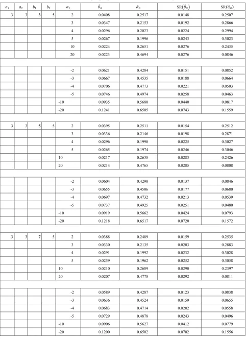
Table 4. 𝑎𝑎1, 𝑎𝑎2, 𝑏𝑏2 are fixed and increase the value of 𝑏𝑏1

3 3 3 5 2 0.0408 0.2517 0.0148 0.2507

3 0.0347 0.2153 0.0192 0.2866

4 0.0296 0.2023 0.0224 0.2994

5 0.0267 0.1996 0.0243 0.3023

10 0.0224 0.2651 0.0276 0.2435

20 0.0223 0.4694 0.0276 0.0846

-2 0.0621 0.4284 0.0151 0.0852

-3 0.0667 0.4535 0.0188 0.0664

-4 0.0706 0.4773 0.0221 0.0503

-5 0.0746 0.4974 0.0258 0.0463

-10 0.0935 0.5680 0.0440 0.0817

-20 0.1241 0.6505 0.0743 0.1559

3 3 5 5 2 0.0395 0.2511 0.0154 0.2512

3 0.0336 0.2146 0.0198 0.2871

4 0.0296 0.1990 0.0225 0.3027

5 0.0265 0.1974 0.0246 0.3046

10 0.0217 0.2658 0.0283 0.2426

20 0.0214 0.4765 0.0285 0.0808

-2 0.0604 0.4290 0.0137 0.0846

-3 0.0655 0.4506 0.0177 0.0680

-4 0.0697 0.4732 0.0213 0.0539

-5 0.0737 0.4925 0.0251 0.0480

-10 0.0919 0.5662 0.0424 0.0793

-20 0.1218 0.6517 0.0720 0.1572

3 3 7 5 2 0.0388 0.2489 0.0159 0.2535

3 0.0330 0.2135 0.0203 0.2883

4 0.0291 0.1992 0.0232 0.3028

5 0.0259 0.1962 0.0252 0.3058

10 0.0210 0.2689 0.0290 0.2397

20 0.0207 0.4778 0.0292 0.0811

-2 0.0589 0.4287 0.0123 0.0838

-3 0.0636 0.4524 0.0159 0.0655

-4 0.0683 0.4714 0.0202 0.0558

-5 0.0729 0.4878 0.0243 0.0496

-10 0.0906 0.5627 0.0412 0.0779

(11)

[image:11.595.67.546.101.603.2]

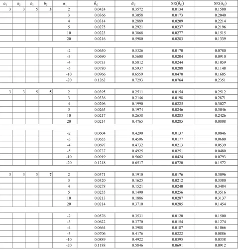
Table 5. 𝑎𝑎1, 𝑎𝑎2, 𝑏𝑏1 are fixed and increase the value of 𝑏𝑏2 .

3 3 5 3 2 0.0424 0.3572 0.0134 0.1580

3 0.0366 0.3058 0.0173 0.2040

4 0.0314 0.2889 0.0209 0.2214

5 0.0275 0.2921 0.0237 0.2196

10 0.0223 0.3868 0.0277 0.1515

20 0.0216 0.5980 0.0283 0.1339

-2 0.0650 0.5326 0.0170 0.0780

-3 0.0690 0.5608 0.0204 0.0910

-4 0.0733 0.5812 0.0244 0.1059

-5 0.0780 0.5937 0.0288 0.1148

-10 0.0966 0.6559 0.0470 0.1685

-20 0.1262 0.7293 0.0764 0.2351

3 3 5 5 2 0.0395 0.2511 0.0154 0.2512

3 0.0336 0.2146 0.0198 0.2871

4 0.0296 0.1990 0.0225 0.3027

5 0.0265 0.1974 0.0246 0.3046

10 0.0217 0.2658 0.0283 0.2426

20 0.0214 0.4765 0.0285 0.0808

-2 0.0604 0.4290 0.0137 0.0846

-3 0.0655 0.4506 0.0177 0.0680

-4 0.0697 0.4732 0.0213 0.0539

-5 0.0737 0.4925 0.0251 0.0480

-10 0.0919 0.5662 0.0424 0.0793

-20 0.1218 0.6517 0.0720 0.1572

3 3 5 7 2 0.0371 0.1910 0.0176 0.3096

3 0.0320 0.1625 0.0212 0.3380

4 0.0278 0.1521 0.0240 0.3484

5 0.0255 0.1490 0.0256 0.3516

10 0.0213 0.1886 0.0287 0.3137

20 0.0214 0.3710 0.0285 0.1454

-2 0.0576 0.3531 0.0120 0.1500

-3 0.0622 0.3770 0.0154 0.1274

-4 0.0664 0.3988 0.0187 0.1066

-5 0.0706 0.4176 0.0222 0.0886

-10 0.0889 0.4922 0.0395 0.0338

-20 0.1188 0.5846 0.0691 0.0912

6. Conclusions

From the Table 1 and 5, we observe the following conclusions.

● For given _𝛼𝛼_, and smaller value of _𝑎𝑎₁, Bayes estimator under GELF is more precise than ML estimates.

● For small value of 𝑎𝑎1 and 𝛼𝛼1 (𝑎𝑎2, 𝑏𝑏1, 𝑏𝑏2 are fixed) , Bayes estimates under GELF is more precise than ML estimates.

● For small value of 𝑎𝑎2 and 𝛼𝛼1 (𝑎𝑎1, 𝑏𝑏1, 𝑏𝑏2 are fixed) , Bayes estimates under GELF is more precise than ML estimates.

● For small value of 𝑏𝑏1 and 𝛼𝛼1 (𝑎𝑎1, 𝑎𝑎2, 𝑏𝑏2 are fixed) , Bayes estimates under GELF is more precise than ML estimates.

● For small value of 𝑏𝑏2 and 𝛼𝛼1 (𝑎𝑎1, 𝑎𝑎2, 𝑏𝑏1 are fixed) , Bayes estimates under GELF is more precise than ML estimates.

We also observe the following conclusions for Bayes estimator:

● For fixed value of 𝑎𝑎1, 𝑎𝑎2 and 𝑏𝑏2 as 𝑏𝑏1 increases, simulated risk of the Bayes estimates under GELF increases.

(12)

REFERENCES

[1] Calabria, R. and Pulcini, G. (1994): An engineering approach to bayes estimation for the Weibull distribution, Micro Electron Reliability, 34, 789 – 802.

[2] Cohen, A. C. (1960): Estimating the parameters of a modified Poisson distribution, JASA, 55, 139 – 143.

[3] Greenwood, M and Yule, G. U. (1920): An enquiry in to the nature of frequency distribution of multiple happenings with particular reference to the occurrence of multiple attacks of disease or repeated accidents, JRSS, Series-A, 83, 255- 279.

[4] Gupta R. C. (1979): Waiting time paradox and size biased sampling. Commun. Stat., Theory Methods A 8 13 , 601 – 607 .

[5] Gupta R. C. (1984): Some characterizations of renewal densities with emphasis in reliability, Math. Operationsforsch. Stat. 15, 571 – 579 .

[6] Gupta R. C., Tripathi R. C. (1987): A comparison between the ordinary and the length – biased modified power series distributions with applications, Commun. Stat., Theory Methods 16, 1195 – 1206 .

[7] Gupta R. C., Tripathi R. C. (1992): Statistical inference based on the length – biased data for the modified power series distributions. Commun. Stat., Theory Methods 21, 519 – 537.

[8] Hassan A., and Ahmad P.B. (2009): Misclassified size – biased modified power series distribution and its applications, Mathematica Bohemica, 134, 1 – 17

[9] Jain G. C. and Consul P. C. (1971): A generalized negative binomial distribution, SIAM J. Appl. Math, 21, 501 – 513.

[10] Jani P. N. and Shah S. M. (1979): Misclassification in modified power series distribution in which the value one is sometimes reported as zero and some of its applications, Metron, XXXVII, N. 3 – 4 , 121 – 136 .

[11] Noack, A. (1950): A class of random variables with discrete distribution, Annals of mathematical statistics, 22, 127 – 132 . [12] Patel A. I., Patel I. D. (2001): Misclassification in modified power series distribution and its applications. Assam statistical Review

15, 55 – 69 .

[13] Patel A. I., Patel I. D (1996): Recurrence relations for moments of the so called misclassified distribution. Assam Statistical Review 10, 107 – 119

[14] Williford W. O., Bingham S. F. (1979): Bayesian Estimation of the parameters in two modified Poisson distributions, Commun Stat., Theory Methods A 8 13 , 1315 – 1326 .