Dictionary Learning for Scalable Sparse Image Representation with Applications

(1)

Dictionary Learning for Scalable Sparse Image

Representation with Applications

Bojana Begovic

∗

,

Vladimir Stankovic

,

Lina Stankovic

Department of Electrical and Electronic Engineering, University of Strathclyde, Glasgow, G1 1XW, UK ∗_{Corresponding Author: [email protected]}

Abstract

This paper introduces a novel design for the dictionary learning algorithm, intended for scalable sparse representation of high motion video sequences and natural images. The proposed algorithm is built upon the foundation of the K-SVD framework originally designed to learn non-scalable dictionaries for natural images. Proposed design is mainly motivated by the main perception characteristic of the Human Visual System (HVS) mechanism. Specifically, its core struc-ture relies on the exploitation of the high-frequency image components and contrast variations in order to achieve visual scene objects identification at all scalable levels. Proposed design is implemented by introducing a semi-random Morphological Component Analysis (MCA) based initialization of the K-SVD dictionary and the regularization of its atom’s update mechanism. In general, dictionary learning for sparse representations leads to state-of-the-art image restora-tion results for several different problems in the field of image processing. In experimental section we show that these are equally achievable by accommodating all dictionary elements to tailor the scalable data representation and reconstruction, hence modeling data that admit sparse representation in a novel manner. Performed simulations include scalable sparse recovery for representation of static and dynamic data changing over time (e.g., video) together with application to denoising and compressive sensing.

Keywords

Scalable Video Representation, Sparse Coding, Regularization, Contrast Variation, Denoising, Compressive Sensing

1 Introduction

Over the past couple of decades, image processing ap-plications have undergone signiﬁcant improvements. A recent critical factor in this growth is the sparse coding paradigm introduced ﬁrstly by [1], based on the assump-tion that signals (e.g., natural images) admit a sparse decomposition over a learned representational basis i.e., dictionary. This so-called sparseland model [2, 3, 4] has led to numerous state-of-the-art algorithms for several

image processing problems [3] speciﬁcally in the con-text of dictionary D ∈ Rn×K _{learning for any image}

signal class. Commonly, the representation of image Y ∈ Rb×b_{, is broken down into a set of} _N _extracted

patches {y_i}N_i₌₁ ∈ Rn _{which are in turn sparsely}

rep-resented. Typically (but not necessarily) it is assumed that dictionary D is overcomplete i.e., the number of its basis vectors (atoms) is greater than the original signal’s dimension (K > n). Given one of the pur-suit algorithms e.g., [5, 6, 7, 8, 9] and a dictionary D, one can estimate matrix X containing sparse approx-imations {xi}

N i=1 ∈ R

K _{for each} _y

i. Hence, a set of

weighted linear combinations of few atoms in D satis-factorily approximates each patchyi ∈Ywith image

de-noted asYb ≈DX. The applications of dictionary learn-ing [10, 11] include areas such as classiﬁcation [12, 13], eﬃcient face recognition [14], inpainiting [15], denoising [16, 17], super-resolution [18, 19], Morphological Com-ponent Analysis (MCA) [20, 21] and those designed for sparse color image processing [22, 23].

In this paper, we provide a detailed presentation of the scalable and sparse modeling dictionary learning frame-work which basic outline was originally presented in [24, 25]. Our focus is placed on designing a procedure for learning a dictionary capable of adapting both to a specific dataset and providing its effective scalable re-construction. Given that current work on scalable data recovery is only based on the the conventional prede-fined dictionaries such as DCT [26] we find that it is important to offer an alternative one in a form of an adaptive dictionary sparse representation. In addition, to the best of our knowledge existing literature just pro-vides the dictionary learning algorithms such as K-SVD [3, 10] that only assume fine resolution as the represen-tational output. This is not sufficient nor tailored to provide the progressive image recovery over its trained sparse representation. Thus, we take and extend the classical form of the K-SVD where the proposed learn-ing scheme differs from the regular one [3, 10] in the sense that:

• Dictionary is initialized in a controlled, semi-random manner using image’s MCA properties [20, 21];

(2)

regular-ization of a dictionary training procedure prior to Singular Value Decomposition (SVD) [27, 28]; • It allows more ﬂexibility for adapting the

scal-able representation to speciﬁc data by removing constraints originally imposed on redundant atoms (i.e., mutually coherent or rarely used) in [5]; • A ﬁrm spatial frequency distribution is enforced

over dictionary atoms as a built in feature;

• OMP pursuing algorithm is replaced via a simple matrix inversion for sparse coefficient estimation given that proposed dictionary is complete. Specifically, proposed implementation is carried out by introducing regularization of the K-SVD atoms update stage aiming for scalable sparse image reconstruction which would improve gradually as we take more and more entries per each coefficient xi ∈ X to restore

{y_i}N_i₌₁ patches. In particular, we emphasize the pe-nalization of the low and high spatial frequency compo-nents of the image patches and dictionary, imposing the learning model that mimics the main HVS [29, 30] sys-tem properties. That is, incorporating HVS’s high sen-sitivity to contrast light information and to the patterns orientation [31, 32] at high spatial frequencies (originally shown via contrast sensitivity function map [33, 34]). The HVS features are proven to be essential modeling elements for many image processing algorithms [35] and image quality assessment tools [36, 37].

Furthermore, in modern video broadcasting networks, an image or a video source is transmitted to numerous clients with various receiver characteristics. These con-sumers differ primarily in accessible: (i) channel capac-ity; (ii) display resolutions; (ii) computing resources. The interesting question is how to support and deliver a controlled quality of the displayed data of a wide range of applications that differ in the users equipment hetero-geneity, communication channels and QoS demands? It would be appealing somehow for a video or image signal to be processed in a such manner that would enable its optimal usability by all diverse clients. For example, the limited frequency space shared by mobile video stream-ing users would be effectively exploited by a generic scal-able i.e., progressive data reconstruction such as pro-posed here. In other words, progressive reconstruction framework would be applied on the source signal prior to its transmission producing its scaled representation form. Once delivered at the client side, depending on its technical specifications, signal would be restored at different quality levels. Thus, signal’s generic scalabil-ity is desirable in many applications since it will be able to support heterogeneity in users equipment, QoS de-mands, and communication channels.

This paper makes following contributions:

1. It tackles for the ﬁrst time the problem of creating a dictionary tailored toscalable image restoration, oﬀering a novel model for data that admits sparse representation;

2. Enforces speciﬁc spatial frequency distribution as a built-in feature over trained dictionary;

3. As a solution to thescalableimage restoration prob-lem, this paper provides an extension and upgrade of the K-SVD dictionary learning concept from non-scalable to scalable adaptive image reconstruction by introducing semi-random dictionary initializa-tion based on the MCA activity norm [3] and by regularizing the learning process of dictionary ele-ments overall promoting the HVS perceptual mech-anism features;

4. The potential of the proposed method is shown for the adaptivescalable denoising and CS;

Evaluation of the scalable recovery is done using high-motion test video sequences and several natural images, successfully attaining progressive frame-to-frame and image scalable restoration. Experimental results con-firm that the proposedscalablescheme outperforms sig-nificantly conventional K-SVD at different scalable im-age recovery levels. Specifically, in terms of application, our focus is placed on applying our proposed scalable scheme to denoising [15] and compressive sensing (CS) [5, 38, 39, 40, 41]. Mainly, in relation to denoising, we tackle processing and computational demands of the [16] given that experimental results in [42] suggest that ob-jective quality improvement of current state-of-the-art image denoising schemes cannot be improved by more than 0.1 [dB]. This conclusion is a result of comparison between the lowest error rates given a simple statistical measure derived from a huge image patch distribution [42] and the empirical errors of state-of-the-art denois-ing algorithms. Lastly, given the CS results in [43, 44] we test the performance of proposedscalabledictionary learning method in one of the CS sampling scenarios.

2 Problem statement and

pro-posed approach

Adhering closely to the notation used in [10], this sec-tion provides the detailed descripsec-tion of the proposed dictionary learning scheme for scalable image recon-struction. We build on the regular K-SVD algorithm [10] by altering its initialization and atom’s update step. In general, we are given a set of N signals i.e., over-lapping image patches of size √n×√n vectorized as Y = [y1, . . . ,yN]∈ Rn×N. The classical conﬁguration

of the K-SVD algorithm aims to approximate represen-tation of these signals in a sparse way as weighted lin-ear combinations of a few dictionary elements i.e., the columns of matrixD= [d1, . . . ,dK]∈Rn×K.

Note however that this conventional approach is not capable of providing scalable image reconstruc-tion that would be based on progressive recovery of each image patch yi. For instance, one can form

{a|1≤a≤ ⌊K/m⌋=s} number of recovery layers for each patch leading to reconstructed image denoted as La. In general,mcan vary and take on diﬀerent values

i.e., 1 < m ≤ K resulting in a number of scalable re-covery layers having m as the scaling parameter. This leads to a progressive image restoration provided as a sequence ofLa image layers each generated as a

(3)

recovery, the base layer L1 is rebuilt out of the ﬁrst m

sparse coeﬃcients entries per patch. That is, for each patch i we take [xi[1] xi[2]...xi[m]] while remaining

entries are set to zeroxi = 0 form < i≤K. These are

combined together with the ﬁrstmcorresponding atoms i.e. [d1,d2, ...,dm] leading to a compression rate ofm/n.

Afterwords, while reconstructing each subsequent layer La (a > 1) additional m coeﬃcients are added. That

is, [xi[1] xi[2]... xi[am]] (xi= 0 foram < i≤K) and

[d1,d2, ...,dam] producing compression ratio of (ma)/n.

The way in which we achieve eﬀective sparse adaptive scalable image reconstruction is by introducing:

1. MCA based semi-random initialization of the dic-tionary at the very beginning of the training proce-dure;

2. A regularization scheme over the second K-SVD iterative stage i.e., the dictionary atom’s update which enforces signiﬁcance of the high frequency components during the regularized atom’s update. The following terms will be used in the remainder of this paper:

• Y ∈ Rn×N - matrix with N overlapping image patchesyi∈Rn;

• Dsc∈Rn×K - proposedscalable dictionary;

• D ∈ Rn×K _{- conventional non-scalable dictionary}

obtained using standard K-SVD [1][5];

• K - the number of dictionary atoms inDscor D;

• X∈RK×N _{- sparse matrix with sparse coeﬃcient}

vectorsxi∈RK.

2.1 Dictionary initialization

In classical K-SVD, prior to any of the two training stages, dictionaryDis initialized with K randomly ex-tracted image training patches yi [10] from the set of

total N. In contrast, prior to initialization we divide the N training patches in two classes C1 and C2 each containing smooth and texture image content, respec-tively. As a classiﬁcation criteria we use the activity measure similar to TV norm originally used within the K-SVD MCA setup [3] and deﬁned as:

Activity(yi) = n ∑ j=2 n ∑ k=1

|yi[j, k]−yi[j−1, k]| (1)

+ n ∑ j=1 n ∑ k=2

|yi[j, k]−yi[j, k−1]|.

Subsequently,Activityis normalized in a way which sets its range from 0 to 1. These values are reflecting the degree of “smoothness” and “textureness” in each im-age patch [3]. The higher the Activity the higher the level of the texture will be within the patch. Thus, the classification is performed via simple tresholding using heuristically set value A. This value is taken from [3] where it is shown that it provides the best possible clas-sification performance for smooth and texture element separation. Specifically, classifying parameter A indi-cates classification of patches into two classesC1 orC2. That is:

• yi ∈C1 forActivity(yi)≤A;

• yi ∈C2 forActivity(yi)> A.

Thereafter, the ﬁrst K/2 atoms of the proposed dictio-nary Dsc are initialized randomly choosingK/2 image

patches from the C1 class, that is, the smooth group. The rest of the K/2 atoms are randomly picked from theC2 class i.e., the texture group. In this way, we en-force semi random initialization which directly controls and eﬀects the starting dictionary structure by placing low frequencies (smooth image areas) within its ﬁrst half ofdjatoms (1≤j≤K/2) and high ones (texture image

areas) within the last half (K/2 < j ≤ K). In return, this sets a foundation for further design which is orga-nized around applying proposed regularization scheme and subsequently tuning dictionary learning to the main HVS perception characteristic.

2.2 Sparse coding

The ﬁrst of the two iterative dictionary learning stages (sparse coding) is posed as a constraint optimization problem deﬁned in [10] as:

min

X {

∥Y−DX∥2_F

}

s.t. ∀i ∥xi∥0 ≤ T0 (2) given the current estimation of the dictionary Dwhich is kept ﬁxed during this process. The expression ∥xi∥0 accounts for the number of non-zero elements in each vectorxi by the means of thel0 pseudo norm whereT0 impose the top limit on ∥xi∥0. Signal yi ∈ Y (i = 1,

. . . ,N), extracted from the original image, is mapped into its sparse representation xi commonly via OMP

[3, 6]. However, given that we train a complete dic-tionary as proposed, OMP is not needed for the sparse coding step. That is, the exact solution for the scal-able dictionary is attained via simple matrix inversion as xi=D′scyiby maintaining up toT0largest non-zero coeﬃcient entries. Each of K entriesxi[j] corresponds to

one of the atoms dj ∈ Dsc (j=1,. . . ,K) where nonzero

entry xi[j]̸= 0 means that particular atom dj

partici-pates in the sparse representation of the signal yi [10].

We relax the sparsity constraint, permitting T0 to take a higher value than in [10] where the relation T0 << n is still maintained. This allows thescalablesignal recov-ery to be established while introducing aT0value on an empirical basis that still promotes the sparsity prior of the signal.

2.3 Regularized dictionary update stage

Once stage described in 2.2 is completed, we move to the atom dj update stage. Usually, the new basis

atom is estimated by processing a current representa-tional residual Ej [10] constructed to account for the

error of all N patches when the atomdj is removed:



Y−∑

k̸=j

dkxkT  ₋djxj_T

2

F

= Ej−djxj_T

2

F

(3)

xk

T represents coeﬃcients from the kth row in X(3) [9]

where xk

(4)

for the patchyiincludes atomdk. Prior to update each

atom dj is set to zero while the remaining basis

ele-ments are kept ﬁxed. Subsequently, error matrixEj is

subject to shrinking [10] which results in reduction of her compositional structure to one which only contains error columns of the patches that use dj. Update of

the pair

[

dj,x j T ]

is obtained via SVD decomposition of such interchanged matrix. Shrinking is necessary in order to preserve the sparsity constraint. That is, the new vector xj_T will keep the sparsity property and it is not going to be fully ﬁlled with non-zero entries af-ter subject to SVD. It is performed by identifying all patches that at the moment of the update use atomdj

asωj= {

i|1≤i≤N,xj_T(i)̸= 0

}

followed with the for-mation of the matrix Ωj size N × |ωj|. This matrix

contains ones only at the (ω(i), i) positions. Remain-ing entries are zeros. MultiplyRemain-ing (3) with Ωj achieves

necessary shrinking.

However, as already stated, this is insuﬃcient to gen-erate dictionary tailored for the scalable image restora-tion. That is why we decide to redeﬁne the structure of theEj (3) by introducing the regularization scheme.

The proposed procedure is mainly motivated by the HVS functional mechanism properties. Specifically, human eyes tend to pay more attention to the edges of an ob-ject given the high firing rate of the visual cortex neu-rons at the moment of perception, primarily identifying objects by their bounding shapes [31, 32]. Thus, in or-der to facilitate effectivescalable recovery, we find that it is necessary to ensure that the main object shapes are identified from the beginning of the image recon-struction. This effect would resemble to some extent to the object recognition procedures [35] which mostly rely on exploitation of image’s high frequency information for this task. Hence, spatial higher frequencies should be more relevant to scalable dictionary learning. We address this by appropriately favoring the significant changes associated with the edges in the image patches (i.e., the texture) during theDsc training. This is

car-ried out by dividing the current sparse approximations of all patches inEj (3) as:

ERj =  Y−v0

K

2 ∑

k=1

dkxkT−v1

K ∑

k=K

2+1

dkxkT 

Ωj, k̸=j.

(4) SuperscriptRstands for regularized and pair [v0, v1] de-notes regularization terms. Each batch corresponds to the low and high frequency components of the training image patches:

• First batch (withv0) contains only atoms initialized from theC1 smooth class;

• Second batch (withv1) contains only atoms initial-ized from theC2 texture class.

This separation is plausible due to semi-random initial-ization described in Sec. 2.1. Proposed design is a result of testing various weight pairs [v0, v1] under the con-straintv0+v1 = 1 in order to avoid degeneracy of the learned representation. Outcomes show that carefully introduced regularization over the smooth and texture

image components is able to yield the appropriate dic-tionary for thescalable data representation (Sec. 3).

Further, by introducing: • Yj =YΩj

• Dlow

sc Xlowj = (∑K/2

k=1dkxkT )

Ωj;

• Dhigh sc X

high

j =

(∑K

k=K/2+1dkxkT )

Ωj;

the proposed regularized error matrix (4) can be rear-ranged as:

ER_j =

(

Yj−v0Dlowsc X low j −v1D

high sc X high j ) (5) where Yj represents a subset of the image patches yi

from Ywith indices given in ωj. Superscriptslow and

high denote smooth and texture frequency content as-sociated with the weight pair [v0, v1] which regularizes contribution of their residual components to the ER

j.

Consequentially, this separation controls the type of the information used for thedj atom’s update.

For all atomsj= 1, ..., K, the proposed update stage is summarized as:

1. STEP 1 - Allocate corresponding image patches which current sparse approximation given as a lin-ear superposition Dscxi includes atom dj as it is

done in [10], map them accordingly withωj and

de-note as a subset of patches Yj, that is a subset of

sparse coeﬃcientsXj;

2. STEP 2 - In contrast to [10], split each current sparse approximation element xi ∈ Xj (i ∈ ωj),

associated with atomdj, in two parts using binary

vectorsTlow_,_Thigh_∈_RK _as:

• xlow

i =xiTlowand xhighi =xiThigh;

where Tlow_,_Thigh _∈ _RK _{are binary vectors that}

cancel anyxi[l] element forl >K₂ (associated with

the dictionary elements initialized with class C1) andl < K₂ (associated with the dictionary elements initialized with classC2) as follows:

• Tlow_[_l_{] =} {

1 if l≤K

2, 0 if l >K₂.

• Thigh_[_l_{] =} {

0 if l≤ K₂,

1 if l > K

2.

In this way the smooth and texture patch content are extracted ﬁnally asDlowsc Xlowj andD

high sc X

high

j ,

respectively.

3. STEP 3 - After decomposing sparse representation ofYj accordingly form newly proposed

representa-tional residual error termER_j associated with atom dj as (5);

4. STEP 4 - Perform rank-one approximation of ER_j via SVD and set the eigenvector corresponding to the largest eigenvalue as newdjand the|ωj|largest

eigenvalues as the new non-zero entries for thexj_T (as in [10]);

(5)

Proposed regularization plays an important role given that weights v0 and v1 control which spatial frequency content will be joined to the ER

j. Consequently, the

SVD decomposition (STEP 4) generates atoms of the scalable dictionary Dsc based on the information

con-tained withinER_j. By keeping more of the original high frequency info (v1<0.5) and suppressing the lower one (v0 > 0.5) the algorithm regularizes the learning pro-cess which eﬀectively generates dictionary Dsc suitable

forscalablerepresentation. This enables recovery of the basic image objects shapes from the base layer L1 re-sulting in a learning procedure which is tailored to the characteristics of HVS.

2.4 Denoising and scalable dictionary

scheme

Prior to presenting thescalable denoising process, we inspect the way in which noise is removed during the classical K-SVD dictionary training. Commonly, noise is iteratively discarded throughout two stages:

1. While performing sparse coding, OMP stops when the current approximated sparse solution reaches the sphere of radius √nCσ in the patches space. This radius constrains the acceptable level of the recovered noise strength i.e., ∥e∥2₂ ≤Cnσ2_{. Going} bellow this boundary would result in direct noise re-construction where C is a heuristically set constant andσstands for the noise standard deviation; 2. During the dictionary’s atom’s update, noise is

re-moved via SVD decomposition that estimates new “average” direction for each atom least inﬂuenced by the distortion.

The conventional K-VD denoising energy minimization problem [16, 17] is given as:

{ b

xi,Db,ybi }

= arg min

xi,D,yi

λyi−y noisy i 2 2 (6) +∑ i

µi∥xi∥0+

∑

i

∥Dxi−yi∥

2 2

We simplify this complex minimization task by relaxing the regularization process with the introduction of the proposedscalable dictionaryDsc as follows:

arg min

Dsc,yi

λyi−ynoisyi

2

2+

∑

i

∥Dscxi−yi∥

2 2 (7) In (7) we decide to discard the sparse coding phase while merely performing noise removal during thescalable dic-tionary Dsc update. Our detailed study of denoising

scheme in [16, 17] suggests that the initial sparseness level i.e., the average number of the non-zero coefficients nearly stays fixed during the dictionary training in the classical K-SVD setup. That is, the one established af-ter the first OMP sparse coding over the initialized dic-tionary [16]. Furthermore, we impose assumption that the noise less distorts texture than smooth image com-ponents due to the high-frequency nature of the tex-ture information. Justification for this is provided in Sec. 4.3 where we illustrate how various level of noise distort smooth and texture image blocks based on their

standard deviation estimated before and after noise is introduced.

Thus, we promote the idea that, after the initial ma-trix inversionX=D′scY(substitute for OMP), we could

neglect subsequent ones during the dictionary learn-ing while still obtainlearn-ing a satisfactory denoislearn-ing results given that texture information prevails for the modi-fied dictionary update. For this setup, the coefficient entries xj_T are only updated during the SVD decom-position employed for the atom’s update. Hence, the introduced modification is expected to result in a con-siderably shorter computational processing time while achieving comparable quality as obtained with the non-scalable K-SVD denoising scheme.

2.5 Computational Complexity

The proposed design does not incur the cost of the original dictionary learning in [3, 10] in case of train-ing strictly representative dictionary over the noise free image. Given that there are no additional transforms employed but just linear separation of the low and high frequencies components via semi-random initialization and introduced error matrix regularization (as shown in Sec. 2.3) the computational complexity remains of the same order as that of the conventional non-scalable K-SVD. That is, the number of operations per pixel is still

O(nT0I) where I stands for the number of iterations. By setting the number of atoms K = n and replacing OMP via simple matrix inversion, we manage to even decrease the processing demands while achieving good signal recovery (typically in [3, 10]K is equal to 2n, 3n

or 4n). This is in particular transparent in relation to when applying proposed scheme to denoising given that sparse coding stage is removed. More details on process-ing time necessary for denoisprocess-ing are shown in Sec. 3.2.

3 Simulation results

The performance of the proposed scalable K-SVD method is evaluated in the set of experiments applied to:

• Standard CIF high motion video test sequences “Stephan” and “Tempete” at resolution 352×288 and a frame rate of 30Hz;

• Several natural images e.g,, “Boat” and “Peppers”, size 512×512.

Variables and parameters for all simulations are sum-marized in Tab. 1 together with their values and roles. Prior to processing, every frame is broken down into

N = 96,945 or every natural image intoN = 255,025 overlapping patches size 8×8 pixels. Thus, the vector-ized dimension of the signals used for the scalable dic-tionary learning algorithm is n= 64 pixels, while both dictionaries Dsc and D containK =n atoms with

(6)

The number of progressively recovered layers La is

de-ﬁned with scaling parameterm= 4 as⌊K/m⌋=s= 16 for every layer of scalable patch recovery and therefore image witha=1, ...,16.

Starting from the first scalable version of the pro-cessed image i.e., base layer L1, the reconstruction is carried out using only first m = 4 entries (i.e., 6.25%) per each sparse coefficient xi. This first level of

trun-cated coeﬃcients fromXis denoted withX1∈R(4)×N. Along this, we employ a truncated version of trained dictionary Dsc: D1sc with only ﬁrst m=4 atoms i.e.,

[d1d2d3d4]. The remaining recovery levels are progres-sively enhanced by adding four (i.e.,m) additional en-tries in each representational vector and four (i.e., m) additional atoms. In general, (for anymvalue) the pro-gressive recovery of the each image patch yi for new

scalable layer La starts by ﬁrst taking all m(a−1)

en-tries from the associated sparse coeﬃcientxi previously

employed for the estimation of theyiscalable version at

the levelLa−1. This continues by adding subsequentm

values from the sparse coeﬃcients xi that are indexed

as:

• x[m(a−1) + 1]_i; • x[m(a−1) + 2]_i; • . . .

• x[m(a−1) +m]_i

with reconstruction for scalable patch at La given as

Dma_sc xma_i withxma_i ∈Xma. The end result is that each recovered patch at the new layerLawill contain the ﬁrst

m(a−1) reconstructed elements as patches inLa−1and newly estimated m. For shown case, this is done un-til the ﬁnal L16 restoration level is attained using full sparse representationX16 =Xand all atoms in dictio-naryD16

sc =Dsc. That is, the recovery scheme for each

image layer is given as:

• L1=D1scX1: 4 atoms and entries per sparse

coeﬃ-cient;

• L2=D2scX2: 8 atoms and entries per sparse

coeﬃ-cient; • . . .;

• L15 = D15scX15: 60 atoms and entries per sparse

coeﬃcient;

• L16 = D16scX16: 64 atoms and entries per sparse coeﬃcient.

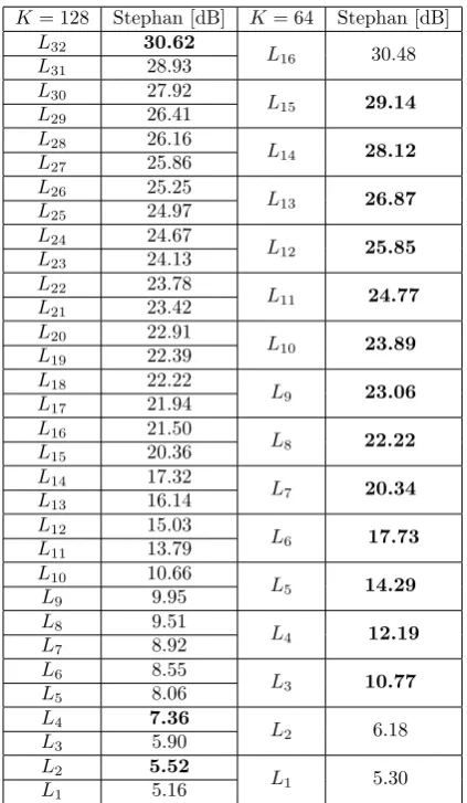
Unlike the classical, non-scalable sparse dictionary learning where practice is to train an overcomplete dic-tionary (K >> n,r >1), we promote training of a com-plete one. One of the main reasons for this arises from our observation that whether we train a complete or overcomplete basis Dsc, the achieved restoration

qual-ity for scalable image representation is highly compa-rable. Tab. 2 and Tab. 3 show the averaged compar-ison at ever scalable recovery level La given the

com-plete and overcomcom-plete scalable scheme for video se-quence “Stephan” and image “Peppers”, respectively. The number of atoms for the overcompleteDsc

dictio-nary is K = 128 (r = 2) thus having greater number

of the recovery levels ⌊K/m⌋ = s = 32 than with the complete scheme given the same scaling factor m = 4. On average, when we take into account all testing re-sults, the diﬀerence of the highest recovered layers i.e.,

L16 goes around 0.15[dB] (for frame size 352×288) and 0.66 [dB] (for image size 512×512) in favor of the over-complete Dsc dictionary. We can see a comparison of

every two recovery levels of the overcomplete Dsc

dic-tionary with one of the recovery level of the complete Dsc in Tab. 2 and Tab. 3 (e.g., L25 and L26 withL13). Conclusion follows that thescalable performance of the complete Dsc overruns the overcomplete Dsc at all

re-covery levels (bold values) except for the ﬁnalL16that isL32for “Stephan” and almost all levels for “Peppers”. Having this in mind together with the fact that lesser number of trained atoms:

• Minimizes the amount of information necessary for training and signal’s recovery;

• Lowers computational complexity;

we choseK= 64. Prior to deﬁning the proposedscalable scheme, we performed exhausting simulations in order to evaluate performance given the variousPiregularization

parameters pairs [v0, v1] listed as: 1. P1: [v0, v1] = [0,1] ;

2. P2: [v0, v1] = [0.1,0.9] ; 3. P3: [v0, v1] = [0.3,0.7] ; 4. P4: [v0, v1] = [0.5,0.5] ; 5. P5: [v0, v1] = [0.7,0.3] ; 6. P6: [v0, v1] = [0.9,0.1] ; 7. P7: [v0, v1] = [1,0] ;

searching for the one which provides the most eﬀective dictionaryDscforscalableimage restoration. Fig. 1 and

Fig. 2 present the averaged PSNR and SSIM estimates at every recovery layerLa ofscalable restoration given the

high motion video sequence “Stephan” and 10 averaged iterations of the natural image “Peppers” withK = 64 number of atoms. As we can see, out of sevenPi

regu-larization (1≤i≤7) scenarios (Fig. 1 and Fig. 2), the

P7results with the dictionary that is most eﬀectively tai-lored to the scalable sparse image representation given that, overall, results with the highest PSNR and SSIM restoration values. Similar results are achieved for video sequence “Tempete” and several other natural images such as “Boat”. For each of the testing,Activity mea-sure is set to the A = 0.27 as in [3]. In addition, we provide results in Fig. 3 (PSNR) and Fig. 4 (SSIM) for all Pi regularization variations when training

overcom-pleteDsc dictionary again with K= 128 atoms for the

K/m = 32 number of La recovery levels. Again, P7 achieves most optimalscalable recovery performance.

To reiterate, the v0 is associated with the Dlowsc

(7)

[image:7.595.125.487.70.212.2]

Table 1. Table of parameters

Parameter Definition Role

N= 96,945 Number of image patches Limits the size of the training set for frames size 352_×288

N= 255,025 Number of image patches Limits the size of the training set for images size 512_×512

n= 64 Constant integer Dimension of image patch vector and each atom

K=64 Number of dictionary atoms Limits the size of the representational basis

K/n=r= 1 Redundancy factor Deﬁnes overcompleteness of the dictionary

v0=1 1stregularization parameter Weights smooth pathc spare presentation for the atom’s update

v1=0 2stregularization parameter Weights texture patch spare presentation for the atom’s update

A= 0.27 Activity measure Classiﬁcation threshold for smooth and texture image patchesyi

T0=10 Sparsity level Limits the number of non zero entries per sparse coeﬃcientxi

l∈ {1, . . . ,64} Integer index Deﬁnes the entry for a sparse coeﬃcientxi

m= 4 Scaling parameter Deﬁnes number ofscalablelayers

⌊K/m⌋=s= 16 General scalability level Total number of thescalablelayers

L= 9 CS scalability level Limits number of thescalablerecovery layers for CS setup

s1< s2, . . . , < sL Progressive CS samples Limit number of samples per each CSscalablerecovery layer

S=sL= 50 Maximal CS sample Limits total number of the CS samples

of theDhigh

sc atoms that contain higher spatial

frequen-cies, that is, the areas of high detail with many contrast-ing edges such as the audience in “Stephan” or the ﬂower object in “Tempete”. By looking at (5) in Sec. 2.3, with

P7 parametrization ([v0, v1] = [1,0]), we can conclude that the regularization process will in each iteration:

• Discard texture sparse approximation Dhigh sc X

high j

given thev1= 0;

• Keep the smooth partDlow_sc Xlow_j withv0= 1. This will determine the ﬁnal content of the regu-larized error matrix ER

j where the texture patches

Table 2. Averaged PSNR quality assessment for scalable restora-tion given the “Stephan” video sequence for two sizes dicrestora-tionary,

K= 64 andK= 128.

K= 128 Stephan [dB] K= 64 Stephan [dB]

L32 30.62 L16 30.48 L31 28.93 L30 27.92 L15 29.14 L29 26.41 L28 26.16 L14 28.12 L27 25.86 L26 25.25 L13 26.87 L25 24.97 L24 24.67 L12 25.85 L23 24.13 L22 23.78 L11 24.77 L21 23.42 L20 22.91 L10 23.89 L19 22.39 L18 22.22 L9 23.06 L17 21.94 L16 21.50 L8 22.22 L15 20.36 L14 17.32 L7 20.34 L13 16.14 L12 15.03 L6 17.73 L11 13.79 L10 10.66 L5 14.29 L9 9.95 L8 9.51 L4 12.19 L7 8.92 L6 8.55 L3 10.77 L5 8.06 L4 7.36 L2 6.18 L3 5.90 L2 5.52 L1 5.30 L1 5.16

(Activity(yi) > 0.27) are dominant information being

directly included into the error synthesis rather than be-ing just a part of the representational residual as the smooth one (Activity(yi)≤0.27). Furthermore, Sec. 4

provides a detailed discussion on eﬀective structural dif-ferences between trained dictionaries and how Dsc is

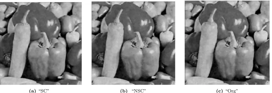
better tailored to the HVS perception system than the non-scalable, conventional dictionary D. Some of these dictionaries are shown in Fig. 5a and Fig. 5b illustrating examples of scalable (“SC K-SVD”) and non-scalable (“NSC K-SVD”) dictionary trained over the ﬁrst frame of the “Stephan” sequence. Given the ﬁrst frame for either of sequences i.e., the training frame, the

intro-Table 3. Averaged PSNR quality assessment for scalable restora-tion given the “Peppers” natural image for two sizes dicrestora-tionary,

K= 64 andK= 128.

K= 128 Peppers [dB] K= 64 Peppers [dB]

[image:7.595.72.284.446.810.2] [image:7.595.326.538.447.812.2]

(8)

[image:8.595.81.490.58.231.2]

(a) “Stephan” video sequence (b)“Peppers” image

Figure 1. Averaged PSNR scalable results given the seven diﬀerent setups for regularization parameters [v0, v1] andK= 64 number of atoms.

Figure 2. Averaged SSIM scalable results given the seven diﬀerent setups for regularization parameters [v0, v1] andK= 64 number of atoms.

duced training scheme is carried out only once generat-ing theDscdictionary. Subsequently, while

reconstruct-ing each incomreconstruct-ing frame we use this sreconstruct-ingleDscthus, not

training any new dictionary. This approach consider-ably reduces the computational complexity of the scal-able sparse video representation, since training is done only once instead for each incoming frame. This is im-mensely important in the context of real-time scalable image/video applications development. It is necessary to mention that in general, when the video scene un-dergoes signiﬁcant changes with respect to thetraining frame, a new training frame should be inserted. This is necessary in order to accommodate for the diﬀerence in the compositional structure of previous frames and newly changed one.

3.1 Scalability Performance

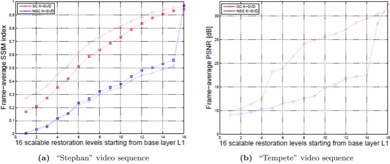
The comparison of the restoration quality is done for the proposed regularizedscalable“SC K-SVD” and con-ventional non-scalable “NSC K-SVD” algorithm. Fig. 6a and Fig. 6b illustrate the PSNR estimates for video se-quences “Stephan” and “Tempete” respectively. Shown results are averaged over all frames given each of 16 recovery {La}

16

a=1 layers. Minor exception is the “Stephan” sequence which frames are divided into two

groups: [1, 270] and [271, 300]. This frame separation is carried out in order to demonstrate the variation in the quality of the restored image, when a new object is introduced in the frame 271. We would expect certain degradation in the restoration quality given thatDsc is

trained over the training frame which does not contain a newly introduced visual object.

Depicted results clearly demonstrate that the pro-posed regularized scheme considerably outperforms the standard [10] over all recovery levelsLa, where average

gain of 11.32 [dB] (“Stephan”, first 270 frames) and 8 [dB] (“Tempete”, all frames) is achieved. This proves superiority of the proposed work in terms ofscalable re-covery. Once a new image object appears (e.g., the ten-nis net in the “Stephan” sequence ) a noticeable drop in thescalablerecovery quality can be noticed in Fig. 6a for the second frame group [271, 300]. Specifically, on aver-age “SC K-SVD” PSNR declines for 1.84 [dB] while still outperforming the “NSC K-SVD” for 9.43 [dB]. Over-all, only in the case when all the information on the sparse coefficients is available (X16∈R(64)×N), the

[image:8.595.88.496.275.447.2]

(9)

[image:9.595.95.504.58.229.2]

Figure 3. Averaged PSNR scalable results given the seven diﬀerent setups for regularization parameters [v0, v1] andK= 128 number of atoms.

[image:9.595.90.504.272.445.2]

Figure 4. Averaged SSIM scalable results given the seven diﬀerent setups for regularization parameters [v0, v1] andK= 128 number of atoms.

(a)“SC K-SVD” (b)“NSC K-SVD”

Figure 5. Scalable and non-scalable dictionaries for the 1st_{“Stephan” frame.}

which image structural information is degraded by cal-culating a quality index ranging from 0 (denoting high-est distortion) up to 1 (denoting no distortion). This measure is specially appealing for the evaluation of the proposed scalable image restoration framework due to the fact that the SSIM is based on the discussed HVS characteristics. Speciﬁcally, it takes into account local pixels distortions of the luminance and contrast informa-tion. The higher the SSIM index value gets, the more successful retrieval of the HVS perception information

at each scalable layerLa will be. This results in a

bet-ter visual information thus providing progressive image recovery of better quality. Therefore, SSIM index values shown in Fig. 7 quantify the degree of the degradation of structural information in a frame at eachscalable recon-struction level La. Once again, these estimates are

[image:9.595.149.461.485.645.2]

(10)

[image:10.595.94.493.60.227.2]

(a) “Stephan” video sequence (b) “Tempete” video sequence

Figure 6. Frame-average PSNR of the scalable reconstructed video test sequences (“Stephan” and “Tempete” ) given for each layer

Laof the scalable video reconstruction using the scalable and non-scalable K-SVD algorithm.

(a) “Stephan” video sequence (b) “Tempete” video sequence

Figure 7. Frame-average SSIM index of the scalable reconstructed video test sequences (“Stephan” and “Tempete” ) given for each layerLaof the scalable video reconstruction using the scalable non-scalable K-SVD algorithm.

group) and 0.28 (second frame group). Similarly, we can see in Fig. 7b, the SSIM diﬀerence of 0.27 for the “Tem-pete” sequence over all recovery levels La between two

dictionary learning algorithms. Interestingly, for SSIM evaluation we have a diﬀerent trend than in the case of PSNR where once we switch to the second frame group the quality assessment shows a high drop for restoration levelsL14, L15, L16. In contrast, Fig. 7a denotes a high similarity in the SSIM values forL14, L15, L16at around 0.94 given both frame groups, meaning that the struc-tural information of the image is preserved despite the fact that we have new visual object in the scene.

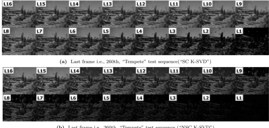
Visualization of the results is provided in Fig. 8, Fig. 9 for “Stephan” and in Fig. 10, Fig. 11 for “Tempete” sequence in order to emphasize the subjective percep-tual quality. These ﬁgures illustrate thescalable recon-struction outcome at every recovery levelLa for the

so-called training frame (Fig. 8 and Fig. 10). The last frames for both video sequences are shown in Fig. 9 and Fig. 11. Here one can observe the visual varia-tions in the restoration quality when the new object containing the high-frequency content structure is in-troduced (i.e., the tennis net in Fig. 9) or the more spatial low-frequencies are added i.e., the background in “Tempete” in Fig. 11. All scalable restorations are performed over the single trained dictionary given the

ﬁrst training frame. From these ﬁgures one can no-tice that the proposedscalable scheme is able to recover the frame at a recovery level L3 (D3sc ∈ R(64)×12 and

X3 ∈ R(12)×N) whereas [1] fails to show any scalable characteristics overall up to L15 (D15sc ∈ R(64)×60 and

X15 ∈R(60)×N_{) for “Stephan” and}_L

8 (D8sc∈R(64)×32

and X8 ∈ R(32)×N_{) for “Tempete”. It should be said}

that the “NSC K-SVD” does show slight scalability with the ”Tempete” sequence. However, this is still far from the performance of the proposed method that keeps its reconstruction eﬃciency consistent for quite diﬀerent video sequences, hence showing its processing stability.

3.2 Application to image processing 1:

denoising

[image:10.595.90.491.275.444.2]

(11)

dictio-(a) Training frame, “Stephan” test sequence (“SC K-SVD”)

[image:11.595.86.524.53.267.2]

(b) Training frame, “Stephan” test sequence (“NSC K-SVD”)

Figure 8. Visual assessment of the scalable reconstruction using the scalable and non-scalable K-SVD at every recovery levelLa.

(a) Last frame i.e., 300th, “Stephan” test sequence (“SC K-SVD”)

[image:11.595.86.529.303.519.2]

(b) Last frame i.e., 300th, “Stephan” test sequence (“NSC K-SVD”)

(a) Training frame, “Tempete” test sequence(“SC K-SVD”)

(b) Training frame, “Tempete” test sequence (“NSC K-SVD”)

[image:11.595.84.525.554.767.2]

(12)

(a) Last frame i.e., 260th, “Tempete” test sequence(“SC K-SVD”)

[image:12.595.67.511.56.268.2]

(b) Last frame i.e., 260th, “Tempete” test sequence (“NSC K-SVD”)

nary is trained for each incoming noisy frame, likewise in [15]. All provided results are averaged over two video se-quences frames i.e., “Stephan” and “Tempete” together with the additional estimates for the several conven-tional images i.e., “Boat” and “Peppers”. For experi-ments we consider the range of ﬁve diﬀerent noise stan-dard deviations: σ = [20,40,60,80,100]. The restora-tion of everyscalable levelLa is carried out in the same

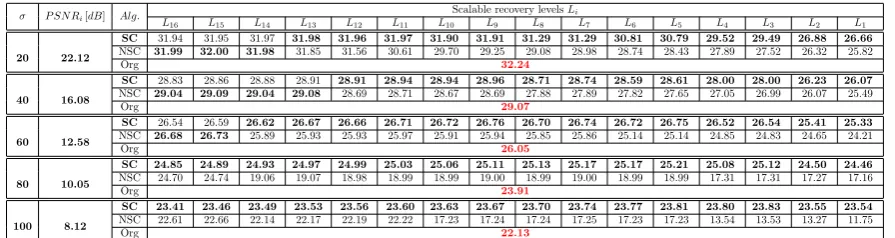
way as in the previous section. Starting from Tab. 4 to Tab. 7 we can see comparison for denoising outcomes at everyscalable recovery layerLa for all mentioned data.

Additionally, each level is compared against the denois-ing estimates of the overcomplete K-SVD scheme “Org” (red, bold values) in order to emphasize the effective-ness of the proposed scheme. From the provided results conclusion follows that PSNR values of the “SC” at the final restoration levelL16(Tab. 4 to Tab. 7) are, at most cases, comparable or surpass (black bold values) denois-ing performance of the classical K-SVD setup once the noise passes valueσ= 60. This better performance in-dicates that the higher frequencies are less influenced by the noise since they are enforced as the most important content of the trained dictionary, contributing most to the restored frame or image unlike in the conventional K-SVD. Overall, the proposed method achieves better denoising performance with lowest and highest gain of 0.1 [dB] and 5.7 [dB], respectively.

In addition, we performed testing for the scenario where the sparse coding stage is also removed from the classical non-scalable K-SVD scheme in order to further validate the practicality of the proposedscalable design. After simulations final estimates show that there is a drop of 2 [dB] for “NSC” without sparse coding stage when compared to the best denoising results of the “SC”. Hence, newly introduced regularization scheme is effi-cient when it comes down to noise removal given that we only keep atom’s update out of two iterative stages for dictionary learning over the corrupted image. The greatest benefit of thescalabledenoising is direct reduc-tion of both, computareduc-tional complexity and processing time where Tab. 8 shows the total denoising run times

in seconds for two image sizes:

1. 352x288 - size of the video sequences frames; 2. 512x512 - size of the conventional images.

Illustrated times are outcomes of processing on the Dell operating system with 64 bit Intel core, 8 GB RAM memory and 2.40 GHz processor. The number of itera-tions for the provided results is ﬁxed and set to sixteen. Based on the averaged run times we can see reduction in:

1. approximately 6.5 times for data of size 352x288 when comparing “SC” vs “Org”;

2. approximately 7.3 times for data of size 512x512 when comparing “SC” vs “Org”;

3. approximately 10.8 times for data of size 352x288 when comparing “SC” vs “NSC”;

4. approximately 11 times for data of size 512x512 when comparing “SC” vs “NSC”;

provided that we achieve still highly comparable (lower levels of noise) or better results (higher levels of noise). The forth column of the Tab. 8 illustrates the time for the error matrix formation per each iteration. These numbers are aiming to show that introduced modiﬁca-tion of the atom’s update in the form of a new error ma-trix scheme inﬂuences processing complexity on a minor scale by being increased on average for two seconds.

(13)

[image:13.595.82.530.71.194.2]

Table 4. PSNR quality assessment for scalable denoising via the scalable and non-scalable K-SVD dictionary, “Stephan” sequence.

σ P SN Ri[dB] Alg.

Scalable recovery levelsLi

L16 L15 L14 L13 L12 L11 L10 L9 L8 L7 L6 L5 L4 L3 L2 L1

20 22.14

SC 28.71 28.73 28.74 28.75 28.71 28.71 28.50 28.47 27.79 27.67 26.37 26.18 24.34 24.13 21.57 21.07 NSC 28.88 28.58 28.22 27.66 26.93 26.57 26.17 25.90 25.39 25.05 24.37 23.97 23.11 22.75 21.08 20.46

Org 29

40 16.13

SC 24.30 24.32 24.34 24.36 24.36 24.38 24.34 24.35 24.18 24.17 23.76 23.71 22.88 22.79 21.02 20.68 NSC 24.64 24.52 24.35 24.09 23.60 23.14 22.84 22.68 22.45 22.28 21.97 21.66 21.17 20.78 20.07 19.51

Org 24.73

60 12.56

SC 21.93 21.96 21.98 22.00 22.01 22.03 22.03 22.05 22.00 22.01 21.86 21.84 21.48 21.45 20.35 20.13 NSC 22.31 22.28 22.13 22.03 21.90 21.87 21.70 21.56 21.38 21.18 21.02 20.86 20.52 20.28 19.70 19.29

Org 22.32

80 10.05

SC 20.49 20.51 20.54 20.56 20.58 20.60 20.61 20.63 20.61 20.63 20.57 20.58 20.41 20.40 19.72 19.58 NSC 20.78 20.79 20.72 20.69 20.66 20.66 20.64 20.61 20.45 20.41 20.30 20.21 19.96 19.79 19.39 19.07

Org 20.75

100 8.13

SC 19.45 19.48 19.52 19.55 19.57 19.60 19.62 19.65 19.66 19.68 19.67 19.68 19.60 19.61 19.17 19.10 NSC 19.63 19.64 19.63 19.64 19.64 19.64 19.60 19.60 19.57 19.55 19.50 19.48 19.35 19.31 18.99 18.77

[image:13.595.83.529.222.342.2]

Org 19.59

Table 5. PSNR quality assessment for scalable denoising via the scalable and non-scalable K-SVD dictionary, “Tempete” sequence.

20 22.12

SC 28.29 28.3 28.21 28.21 28.03 28.02 27.73 27.7 27.27 27.22 26.63 26.55 25.62 25.49 23.86 23.56 NSC 28.27 28.11 27.97 27.81 27.59 27.41 26.99 26.75 26.25 25.97 25.42 25.15 24.52 24.08 23.06 22.56

Org 28.40

40 16.07

SC 24.61 24.63 24.62 24.64 24.61 24.62 24.56 24.56 24.45 24.46 24.28 24.27 23.92 23.88 23.01 22.87 NSC 24.71 24.70 24.64 24.64 24.58 24.49 24.29 24.16 24.08 23.88 23.77 23.51 23.38 22.68 22.20 21.72

Org 24.76

60 12.55

SC 22.59 22.61 22.63 22.65 22.65 22.67 22.66 22.67 22.64 22.66 22.6 22.61 22.48 22.47 22.07 22 NSC 22.59 22.60 22.60 22.60 22.58 22.58 22.53 22.51 22.44 22.41 22.29 22.23 21.96 21.85 21.51 21.23

Org 22.52

80 10.07

SC 21.18 21.2 21.23 21.25 21.27 21.29 21.3 21.32 21.32 21.34 21.33 21.34 21.3 21.3 21.13 21.11 NSC 21.12 20.32 20.19 19.35 17.94 15.79 15.32 15.29 15.06 14.10 14.00 13.75 13.72 12.22 12.18 11.62

Org 21.01

100 8.14

SC 20.04 20.07 20.09 20.12 20.14 20.17 20.18 20.21 20.22 20.25 20.26 20.28 20.27 20.28 20.22 20.22 NSC 19.92 19.65 18.72 17.86 16.61 16.01 15.35 14.23 13.65 13.63 13.36 12.68 11.92 11.38 11.12 10.92

[image:13.595.80.532.372.493.2]

Org 19.69

Table 6. PSNR quality assessment for scalable denoising via the scalable and non-scalable K-SVD dictionary, “Boat” image.

σ P SN Ri[dB] Alg. Scalable recovery levelsLi

20 22.11

SC 30.13 30.14 30.01 30.02 29.82 29.82 29.49 29.49 28.94 28.94 28.06 28.06 26.60 26.59 24.57 24.55 NSC 30.31 30.26 30.14 30.02 29.79 29.59 29.31 29.04 28.67 28.40 27.75 27.29 26.39 26.01 24.50 24.15

Org 30.52

40 16.09

SC 26.80 26.83 26.81 26.84 26.80 26.82 26.74 26.76 26.60 26.62 26.25 26.26 25.47 25.48 24.05 24.06 NSC 27.11 27.13 27.09 27.09 26.91 26.87 26.72 26.56 26.32 26.23 25.88 25.84 25.24 24.83 24.04 23.71

Org 27.11

60 12.55

SC 24.86 24.89 24.90 24.93 24.94 24.97 24.95 24.98 24.93 24.96 24.80 24.82 24.39 24.41 23.49 23.51 NSC 25.11 25.15 25.13 25.16 25.10 25.12 25.04 25.05 24.87 24.88 24.70 24.68 24.23 24.12 23.54 23.34

Org 25.02

80 10.05

SC 23.46 23.50 23.53 23.56 23.58 23.62 23.63 23.67 23.66 23.69 23.62 23.65 23.42 23.45 22.89 22.92 NSC 23.59 23.63 23.65 23.68 23.69 23.73 23.70 23.73 23.65 23.68 23.57 23.59 23.31 23.32 22.94 22.88

Org 22.83

100 8.15

SC 22.37 22.41 22.44 22.48 22.51 22.55 22.57 22.61 22.62 22.66 22.63 22.67 22.53 22.56 22.22 22.26 NSC 22.43 22.48 22.52 22.57 22.59 22.63 22.61 22.63 22.62 22.65 22.58 22.60 22.46 22.46 22.22 22.21

Org 21.46

Table 7. PSNR quality assessment for scalable denoising via the scalable and non-scalable K-SVD dictionary, “Peppers” image.

20 22.12

SC 31.94 31.95 31.97 31.98 31.96 31.97 31.90 31.91 31.29 31.29 30.81 30.79 29.52 29.49 26.88 26.66 NSC 31.99 32.00 31.98 31.85 31.56 30.61 29.70 29.25 29.08 28.98 28.74 28.43 27.89 27.52 26.32 25.82

Org 32.24

40 16.08

SC 28.83 28.86 28.88 28.91 28.91 28.94 28.94 28.96 28.71 28.74 28.59 28.61 28.00 28.00 26.23 26.07 NSC 29.04 29.09 29.04 29.08 28.69 28.71 28.67 28.69 27.88 27.89 27.82 27.65 27.05 26.99 26.07 25.49

Org 29.07

60 12.58

SC 26.54 26.59 26.62 26.67 26.66 26.71 26.72 26.76 26.70 26.74 26.72 26.75 26.52 26.54 25.41 25.33 NSC 26.68 26.73 25.89 25.93 25.93 25.97 25.91 25.94 25.85 25.86 25.14 25.14 24.85 24.83 24.65 24.21

Org 26.05

80 10.05

SC 24.85 24.89 24.93 24.97 24.99 25.03 25.06 25.11 25.13 25.17 25.17 25.21 25.08 25.12 24.50 24.46 NSC 24.70 24.74 19.06 19.07 18.98 18.99 18.99 19.00 18.99 19.00 18.99 18.99 17.31 17.31 17.27 17.16

Org 23.91

100 8.12

SC 23.41 23.46 23.49 23.53 23.56 23.60 23.63 23.67 23.70 23.74 23.77 23.81 23.80 23.83 23.55 23.54 NSC 22.61 22.66 22.14 22.17 22.19 22.22 17.23 17.24 17.24 17.25 17.23 17.23 13.54 13.53 13.27 11.75

Org 22.13

Table 8. Comparison of the processing time given tree denoising schemes

Image size Alg. Total denoising run time [s] Error formation time [s]

352x288

Org 2897.6 1.26

NCS 3515.7 2.61

SC 325.1 4.42

512x512

Org 7565.5 1.59

NCS 7337.3 1.58

SC 665.5 3.29

3.3 Application to image processing 2:

compressive sensing

Following closely the experimental layout suggested in [26], we investigate the eﬀectiveness and the

[image:13.595.82.530.522.641.2] [image:13.595.184.429.671.734.2]

(14)

[image:14.595.59.521.56.192.2]

recov-(a)“SC” (b) “NSC” (c)“Org”

Figure 12. Visual assessment for denoising via the scalable, non-scalable complete and over complete K-SVD atL16recovery level of the ﬁrsttrainingframe of the “Stephan” video sequence,σ= 40

[image:14.595.56.522.235.369.2]

(a)“SC” (b) “NSC” (c)“Org”

Figure 13. Visual assessment for denoising via the scalable, non-scalable complete and over complete K-SVD atL16recovery level of the ﬁrsttrainingframe of the “Tempete” video sequence,σ= 40

(a)“SC” (b) “NSC” (c)“Org”

Figure 14. Visual assessment for denoising via the scalable, non-scalable complete and over complete K-SVD at L16 recovery level given the image “Boat”,σ= 40

ery while analysing the implications of the sub-Nyquist CS paradigm in both the scalable and adaptive repre-sentational domain. Likewise in previous experimental sections and as in [26], the image is processed block by block. Mainly, we take into consideration two cases of the CSscalable recovery:

• With the proposed scalable K-SVD dictionary tai-lored to this task;

• With the conventional non-scalable K-SVD dictio-nary.

[image:14.595.56.524.412.573.2]

Rather than taking the full number of measurements [5, 45, 46] over every incoming frame, CS sampling is carried out in incremental steps. Note that this is appli-cable only for the CS scalable sensing scenario. Given

the suﬃcient number of progressive measurements per patch ass1,s2, . . . ,sL(si< n) we are able to recover the

frame gradually after incrementally retrieving entries of sparse vector coeﬃcients in Xi via OMP. Furthermore,

each incremental number of samplessi satisﬁes the

fun-damental result of the CS theory [2] that imposes the limit on the necessary number of measurements for sat-isfactory signal reconstruction.

Unlike the conventional CS for our testing we apply specially structured sampling matrix Φ. This aims to achieve eﬃcientscalableacquisition of samples over each image layer commonly denoted asy_CS=Φy=ΦDscx.

(15)

[image:15.595.77.538.55.214.2]

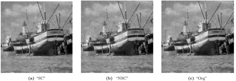
scal-(a)“SC” (b) “NSC” (c)“Org”

Figure 15. Visual assessment for denoising via the scalable, non-scalable complete and over complete K-SVD for theL16recovery level given the image “Peppers”,σ= 40

[image:15.595.105.507.262.434.2]

(a) “Stephan” video sequence (b)“Tempete” video sequence

Figure 16. Frame-average PSNR of the scalable CS reconstruction for two test video sequences as a function of the measurement procent using the scalable (“SC K-SVD”) and non-scalable (“NSC K-SVD”) algorithm.

able task at hand. For each recovery step (as in [26]) we scale sampling matrix size-wise into its truncated ver-sions as Φi ∈ Rsi×n. Once the sampling is done we

attain a group of samples each denoted as yi

CS. The

sampling is structured in a way that the basic level is collected via Φ1 that contains binary entries generated from the Gaussian distribution. Remaining measure-ments are sampled via Bernoulli binary distributed en-tries ofΦi consecutively added up to the basic layer for

the scalable restoration. Again, starting from a base level i = 1 and with y1

CS =Φ1y = Φ1Dscx

(approxi-mately 15% of original patch image sizeyi) we advance

through enhancement layers by uniformly collecting ad-ditional number of samples (e.g., s2, s3, ...,sL = S) in

each step until the total number of S < n samples is reached. Hence, given the single trained dictionaryDsc

(as in Sec. 3.1) learned overtrainingframe for either of video test sequences, one can deﬁne an arbitrary number of sampled layers over extracted image patches.

Fig. 16 shows reconstruction results obtained via the proposed adaptive scalable CS approach averaged over the frames starting withs1 = 10 and adding ﬁve more samples per each patch as frame recovery progresses (e.g.,s2= 15,s3= 20, etc.). Therefore, we deﬁne in to-tal nine sampling levels resulting in nine patch, that is, frame reconstruction layers. Thus, full number of mea-surements isS= 50 (n >50) which accounts for roughly

80% of the information of the sampled signalyi. The gap

between the performance of the two methods is evident for the layers sampled both at low (e.g., 15%, 23% , 31% and 39%) and high subrates (47%, 55%, 62%, 70% and 80%) of sampling information, at around 3.03 [dB] in case of “Stephan” sequence and for the “Tempete” frames at 2.96 [dB]. We can see that the proposed de-sign is successful for the subsampling factors at diﬀerent rates whereas the conventional K-SVD has a compara-ble but not better performance as more measurements are added.

4 Discussion

Training the dictionary for the scalable sparse data representation and applying it to the denoising adopts a diﬀerent approach than the one originally introduced by K-SVD [3, 9, 15]. Mainly, the atom update illustrated in Sec. 2.3 and denoising proposed Sec. 2.5 are grounded in the following assumptions:

• The progressive and quality wise scaled recovery of the image/frame can be attained via learned dictio-nary by modeling the main HVS perception mech-anism properties and integrating them during dic-tionary’s training;

(16)

(a)“Stephan” (b)“Tempete”

[image:16.595.90.498.57.415.2]

(c)“Boat” (d)“Peppers”

Figure 17. Activityatom’s pattern for the dictionaries of the two video sequences and two natural images.

separation and regularization of low and high spa-tial frequencies information captured by the atoms during the dictionary training procedure;

• Texture image components are less distorted by noise than the smooth ones thus with the newly introduced design SVD over proposed regularized error matrixER

j is suﬃcient for noise removal.

These hypotheses give rise to a series of questions: 1. How are spatial frequencies distributed overscalable

and non-scalable dictionary’s atoms?;

2. Could this distribution be denoted as a built-in property of the trained dictionaries?

3. Does the proposed design properly adopt the HVS perception mechanism properties?

4. To what degree noise eﬀects smooth and texture image properties?

The following sections aim to look into some answers to these questions.

4.1 Spatial frequencies distribution

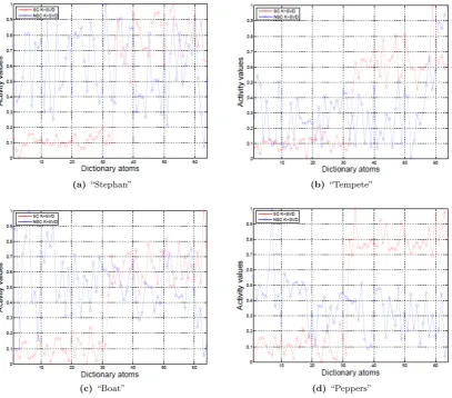
In Sec. 2.1 we gave a detailed explanation on semi-random dictionary initialization where we enforce al-location and separation of the dictionaries atoms into smooth and texture ones. As explained, the classiﬁca-tion criteria we use is formulated viaActivity norm in

[3]. Thus, we further assess the spatial frequencies dis-tributions for both dictionaries by looking at and ana-lyzingActivity trend once the training is done. This is illustrated with Fig. 17. Whether we consider frames of the video sequence (Fig. 17a and Fig. 17b) or some conventional image (Fig. 17c and Fig. 17d) we can con-clude that classical K-SVD scheme results in dictionar-ies which do not show any speciﬁc structural features in terms of how smooth and texture information are learned and allocated. In contrast, proposed design shows clear distinction between atoms that carry:

• Low spatial frequency: Activity(dj) j=K/2

j=1 ≤ A = 0.27 (ﬁrstK/2 atoms);

• High spatial frequency: Activity(dj) j=K

j=K/2 > A= 0.27 (lastK/2 atoms);

thus successfully implementing this speciﬁc distribution as a built-in property of thescalable dictionaryDsc

un-like the classical K-SVD scheme.