Munich Personal RePEc Archive
Real time estimation of potential output
and output gap for theeuro-area:
comparing production function with
unobserved componentsand SVAR
approaches
Lemoine, Matthieu and Mazzi, Gian Luigi and
Monperrus-Veroni, Paola and Reynes, Frédéric
Observatoire Français des Conjonctures Economiques, Eurostat
November 2008
Online at
https://mpra.ub.uni-muenchen.de/13128/
R
EALT
IMEE
STIMATION OFP
OTENTIALO
UTPUT ANDO
UTPUTG
APFOR THE
E
URO-A
REA:
C
OMPARINGP
RODUCTIONF
UNCTION WITHU
NOBSERVEDC
OMPONENTS ANDSVAR
A
PPROACHESN° 2008
–
34
Novembre 2008
Matthieu L
EMOINEOFCE
Gian Luigi MAZZI Eurostat
Paola MONPERRUS-VERONI OFCE
Real time estimation of potential output and output gap for the
euro-area : comparing production function with unobserved components
and SVAR approaches
1Matthieu LEMOINE♠2, Gian Luigi MAZZI♣, Paola MONPERRUS-VERONI♠ and
Frédéric REYNES♠
♠ OFCE - Analysis and Forecasting Department
♣ Eurostat - D1 Key Indicators for European Policies
Abstract
We develop a new version of the production function (PF) approach usually used for estimating the output gap of the euro area. Our version does not call for any (often imprecise) measure of the capital stock and improves the estimation of the trend total factor productivity. We asses this approach by comparing it with two other multivariate methods mostly used for output gap estimates, a multivariate unobserved components (MUC) model and a Structural Vector Auto-Regressive (SVAR) model. The comparison is conducted by relying on assessment criteria such as the concordance of the turning points chronology with a reference one, the inflation forecasting power and the real-time consistency of the estimates.
Two contributions are achieved. Firstly, we take into account data revisions and their impact on the output gap estimates by using vintage datasets coming from the Euro Area Business Cycle (EABCN) Real-Time Data-Base (RTDB). Secondly, the PF approach, generally employed by policy-makers despite of its difficult implementation, is assessed. We thus improve on previous papers which limited their assessment on other multivariate methods, e.g. MUC or SVAR models.
The different methods show different ranks in relation to the three criteria. This new PF estimate appears highly concordant with the reference chronology. Its forecasting power appears favourable only for the shortest horizon (1 month). Finally, the SVAR model appears more consistent in real-time.
JEL codes: C32, E32
Keywords : potential output, production function, state-space models, structural VARs
1
This paper is based on a report for Eurostat : “Real time estimation of potential output, output gap, NAIRU and Phillips curve for Euro-zone”, part of the Advanced statistical and econometric techniques
for the analysis of PEEIs EUROSTAT Project, December 2007
2
Corresponding author: Matthieu Lemoine, OFCE, 69 quai d’Orsay, 75007 Paris, France [email protected]
1. Introduction
Since Okun’s contribution (1962), the concepts of potential GDP (or potential output) and output gap are widely used in macroeconomics even though their definition and estimation raise a number of theoretical and empirical issues. An output gap is defined as the difference between the – unobservable – potential and the actual GDP. Potential output is commonly defined as the “maximum output an economy can sustain without generating a rise in inflation” (De Masi, 1997) or equivalently level of production reached with the full use of disposable production factors.
An accurate measure of the potential output is an important challenge to policy makers in mainly two respects. The first one is related to structural policy recommendations, i.e. all those structural policies likely to enhance potential output and consequently potential growth. Indeed, increasing potential growth may help to solve the sustainability problems of social (health care and pension) systems faced by most OECD countries because of their ageing population. The second one concerns business cycle policy. A level of real output above potential output, i.e. a positive output gap, indicates demand pressures and signals to the monetary authority a possible increase of inflation pressures and that policy tightening may be required.
The output gap interpretation followed by international organizations (OECD, European Commission, ECB…) generally rests on an economic-based approach relying on a production function (PF). Hence, the notion of potential output has clearly-identified theoretical foundations and its estimation relies on non-statistical approaches such as the estimation of a NAIRU or of the parameters of the production function. However, three key issues arise in implementing economic-based PF models. Firstly, information about the underlying economic theory is necessary, but a broad consensus of undisputed and directly useable economic theories can be hardly identified. This remark holds for the specification of the production function and the estimations of the NAIRU and the Phillips curve (Richardson et al., 2000). Secondly, the capital stock is generally not precisely estimated. Thirdly, production function approaches generally involve non-economic-based techniques such as the use of statistical detrending methods, in particular for the estimation of the trend of total factor productivity incorporated in the production function (see for instance Mac Morrow and Röger 2001, Banque de France 2002, de Bandt and Rousseaux 2002). Hence, the PF estimate of the potential output delivers often the same result as a basic statistical filter of the GDP.
In this paper, we try to improve the PF methodology in three ways simultaneously. Firstly, the general Constant Elasticity of Substitution (CES) specification is assumed, instead of the Cobb-Douglas one. Secondly, we decompose GDP into labour and labour productivity thus avoiding the use of an imprecise measure of the capital stock. The labour / capital substitution is taken into account via
The PF approach remains dominant in structural analysis but it has been challenged by other methods in the business cycle analysis because of its difficulties of implementation. We compare the business cycle analysis performances of our proposed PF methodology with those of two other multivariate methods applied to GDP, the inflation and the unemployment rate: a multivariate unobserved components (MUC) model and a Structural Vector Auto-Regressive (SVAR) model. The assessment criteria are the concordance of the turning points chronology with a reference one, the forecasting power regarding inflation and the real-time consistency of the estimates.
The real-time consistency cannot be used as a unique criterion, because a constant estimate of the output gap would perform optimally according to this criterion but very poorly according to the concordance criterion. Nevertheless, the real-time aspect is particularly important in the business cycle analysis, because policy-makers are more interested in the current value of the output gap at each date than in its past and revised values. Orphanides and Van Norden (2002) have shown with US data that the output gap is unreliable in real-time, when a univariate method is used for its estimation. For the euro area, multivariate methods provide more reliable estimates in quasi real-time, i.e. using at each date only the past and current observations from the last version of the dataset (Camba-Mendez and Rodriguez-Palenzuela, 2003).
In this paper, two contributions are achieved. Firstly, the assessment of output gap estimates for the euro area relies on the real-time vintages of the data and not on a final version of the data. Data revisions and their impact on the output gap estimates are taken into account. The vintages come from the Euro Area Business Cycle (EABCN) Real-Time Data-Base (RTDB). Secondly, the PF approach, generally followed by policy-makers and international organizations despite of its difficult implementation, is assessed. We improve on previous papers which limited the assessment to other multivariate methods, e.g. MUC or SVAR models.
Section 2 presents alternative specifications of multivariate empirical models for the estimation of potential output and of the output gap, namely a production-function-based model, a multivariate unobserved model and a structural VAR model. Econometric estimations of the output gap and of the NAIRU with each model are provided in Section 3. Section 4 studies the real-time properties and the stability of such models, by estimating them in real-time and quasi-real-time. An Hodrick-Prescott filter is used as a benchmark. Section 5 concludes showing advantages and drawbacks of the different approaches in relation to the specific goals of structural analysis, business cycle analysis, policy-making and forecasting.
2. Alternative specifications of empirical models for the estimation of
potential output, the output gap and the NAIRU
unobserved components model that estimates simultaneously the output gap, a Phillip’s curve and an Okun’s law, and (3) a SVAR model.
2.1 The “model-based” production function approach
The concept of potential output corresponds to the level of production reached with the full use of disposable production factors (generally labour, capital and technical progress). In the production function approach, potential output is formally and theoretically defined from a production function (PF). It is computed after calculating the potential or equilibrium values of each production factor. For instance, the potential labour is a function of the potential value of the population, the labour participation rate and the unemployment rate. Potential values of the production factors can be obtained either by estimating a theoretical model providing equilibrium values or by filtering each determinant of the output. The former methodology, that we call the “model-based production-function approach” is a pure economic-based one. The latter one, that we call the “statistical PF approach” consists in applying filtering or smoothing techniques such as Hodrick-Prescott (HP) filter to each component: the capital stock, the population, the participation rate, the unemployment rate and the productivity. It more or less delivers the same outcome as if filtering techniques were directly applied to output data. Because of the additivity property of the HP filter, the result is identical as long as the same smoothing parameter is used for all series (see Ongena and Röger, 1997). The statistical PF approach presents the advantage of explaining the contribution to growth from a supply point of view and to be able to decompose the output gap into a capital gap, a population gap, a labour participation gap, an unemployment gap and a productivity gap. But it provides more an explication of past trend output rather than a real estimate of potential output. It therefore presents the same drawbacks of purely statistical approaches.
Major economic institutions such as the OECD (Beffy et al., 2007), the European Central Bank (Denis et al., 2006) and the European Commission (Cahn and Saint-Guilhem, 2007) currently use “hybrid” approaches which combine the model-based and the statistical production function approaches. In most cases, the potential technical progress and the potential labour force are estimated using filtering techniques, whereas the NAIRU is estimated simultaneously with a Philips curve relation.
The specification of the production function generally retains two simplifying hypothesis (see for instance by Rünstler, 2002 and Proietti et al. 2002). Firstly, constant-returns to scale are assumed so that a 1%-increase in production factor leads to a 1%-increase in output. Secondly, the technology is often represented as a Cobb-Douglas function. In particular, the Cobb-Cobb-Douglas technology has been widely used by the major economic institutions (see Giorno et al., 1995; CEPII, 1997) and is currently used by the OECD (Beffy et al., 2007), the European Central Bank (Cahn and Saint-Guilhem, 2007) and the European Commission (Denis et al., 2006). The standard PF approach based on a Cobb-Douglas technology offers the advantage of allowing for a straightforward decomposition of production and hence of easily allowing for the calculation of the contribution of production factors (employment, capital and total factor productivity) to growth, but it presents mainly three drawbacks:
(2) It has to overcome the difficulty of providing a proper estimation of the stock of capital. The capital stock is generally computed as the accumulation of quarterly national account investment flows by assuming an ad hoc constant rate of capital depreciation, although several corrections are sometimes introduced. The European Central Bank (ECB) corrects for the degree of excess capacity in capital whereas the OECD corrects by differencing capital by age/efficiency profile.
(3) It hardly provides a proper estimation of the Total Factor Productivity (TFP). Technical progress is generally computed as a residual by inverting the production function. As this “Solow residual” is extremely erratic, filtering techniques are generally applied which may give poor approximation at the end of the sample. Alternatively, the ECB study (Cahn and Saint-Guilhem, 2007) estimates econometrically the TFP as a determinist trend. This latter approach is unsatisfactory since it assumes that the TPF trend is constant over time which makes difficult to calculate the level of potential output. Indeed, it leads to downward (resp. upward) bias in the potential output estimate in times of acceleration (slowdown) of the TFP. This outcome can explain why only potential output growth is computed in the ECB study.
In this paper, we propose a methodology that aims at overcoming these three shortcomings:
(1) We relax the constraint of unit elasticity of substitution between labour and capital by estimating a labour productivity equation deduced from a Constant Elasticity of Substitution (CES) production function.
(2) Using the definition that output is the product of labour and of labour productivity, we do not need to estimate the stock of capital in order to calculate potential output. At the same time, labour-to-capital substitution is taken into account via the impact of the relative cost between labour and capital on labour productivity.
(3) As an alternative to univariate filtering of the “Solow residual” or to the econometric estimates of the TFP as a determinist trend, a Time-Varying (TV) - coefficients econometric method (the Kalman filter) is used to estimate technical progress simultaneously with the labour-capital substitution ratio and the cyclical components of labour productivity. This method is also used to estimate the NAIRU simultaneously with a Phillips curve and to estimate trend labour participation taking into account discouraged-worker effects. Here as well, a TV trend is more realistic than a determinist trend, since the labour participation ratio has an upper and a lower bound.
By definition, output (Y) can be linearly decomposed into labour productivity ( rod
P ) and employment (N), which can itself be linearly decomposed into the working age population (Pop), the labour market participation rate (Part) and the unemployment rate (U) 3:
3
rod op part rod
y= +n p = p + p − +U p (1) This decomposition allows for the identification of the determinants of potential
output, namely the equilibrium or potential value (mentioned with a *) of the population, the labour force participation rate, the unemployment rate and labour productivity:
op art rod
y∗= p ∗+p ∗−U∗+ p ∗ (2) It also allows for a straightforward linear decomposition of the output gap into a
population gap, a labour participation gap, an unemployment gap and a productivity gap:
( op op ) ( art art ) ( ) ( rod rod )
y−y∗ = p −p ∗ + p −p ∗ − U−U∗ + p −p ∗ (3) The potential population is assumed to be the actual population so that the population gap is null. The theoretical foundations of the other determinants are detailed in Appendix A. The potential unemployment is the NAIRU which is simultaneously estimated with an augmented Phillips curve in a space-state model using the Kalman filter4:
(
)
(
)
(
)
1 1 2 2 1 2 3 3
4 1 1 5 2 2 6
1
1
1 ( )
+
C
C C C C
t t t t t t
P
M C M C UR
t t t t t t
t t t
U t t t
P P P P U U
P P P P C
U U U
U U
β β β β β
β β β ε
ε ∗∗ ∗ − − − − − − − ∗ ∗ ∗∗ + ∗∗ ∗∗ + ⎧ = + + − − − − ⎪ ⎪ + − + − + + ⎪ ⎨ − = ⎪ ⎪ = ⎪⎩ (4)
where C
P is the consumer price, M
P the import price, CUR the capacity utilisation
ratio. pC t
ε and U t
ε ∗∗
are Gaussian independent noises with variances 2 ,PC
ε
σ and
** **
2 2
,U q ,U ,PC
ε ε ε
σ = σ , where qε,U** is the corresponding signal-to-noise ratio.
The potential labour participation is deduced from the estimation of a labour participation equation which takes into account discouraged-worker effects (λ1) via
the negative impact of unemployment on the labour participation ratio:
1
1
art
art
art art P
t t t t
art art art
t t t
P art art
t t t
P P U
P P P
P P λ ε ε ∗ ∗ + ∗ ∗ + ⎧ = − + ⎪⎪ − = ⎨ ⎪ = + ⎪⎩ (5)
where εtPart and εtPart∗ are Gaussian independent noises with variances σε2,Part and
2 2
,Part q ,Part ,Part
ε ε ε
σ ∗ = ∗σ , where qε,Part∗ is the corresponding signal-to-noise ratio.
The trend participation rate (Part) is specified as a Time-Varying (TV) parameter. This hypothesis is far more realistic than the one of a constant deterministic trend traditionally assumed in the literature. Indeed the latter is in contradiction with the fact that the participation rate has an upper and a lower bound: it cannot go below 0 or above 100%.
coefficients are positive. L being the lag operator,
0 ( ) n i i i L L γ γ =
=
∑
is the lag polynomial and γ(1) is thelong-run coefficient. X t
ε is a Gaussian independent noise with variances 2 ,X
ε
σ . For algebraic simplicity, we use the following linear approximation:ln(1+U)≈U.
4
After the estimation of Equation (5), the potential participation rate can be calculated as a function of the trend participation rate and the NAIRU:
art art
t t t
p ∗ = p −λU∗ (6)
Assuming a CES technology with constant returns to scale, the labour productivity equation dissociates the impacts of the technical progress (e), of the relative cost between labour and capital (rc) and of the cyclical component (cycle).
(
)
(
)
1 1 1 *1 2 3 3
1 2 3 3
. .
( )
cos( )( ) sin( )
sin( )( ) cos( )( )
rod
ycle
ycle
p rod c ycle
t t t t t
c r C
t t t t t t
t t t e t t t
c
ycle ycle ycle
t t t t
c
ycle ycle ycle
t t t t
p e r c
r w e p I P
e e e
e e
c c c
c c c
ρ α ε
ε
ρ ρ ρ ε
ρ ρ ρ ε
∗ ∗ ∗ + ∗ ∗ + + ∗ ∗ + ⎧ = + + + ⎪ = − − − − ⎪ ⎪ − = ⎪⎪ ⎨ = + ⎪ ⎪ = + + ⎪ ⎪ = − + + ⎪⎩ (7)
where Wis the compensation per employee, P the GDP price, Ir the interest rate, α the share of value-added going to profit assumed to be equal to 30% and ρ1 the elasticity of substitution between capital and labour. εtprod ,εte∗, εtcycle and εtcycle∗ are Gaussian independent noises with variances σε2,prod ,
2 ,e
ε
σ ∗,
2 ,cycle
ε
σ and
* *
2 2
,cycle q ,cycle ,cycle
ε ε ε
σ = σ , where qε,cycle* is the corresponding signal-to-noise ratio.
Technical progress is specified as a TV parameter in order to capture the evolution of the TPF. Technical progress (e) is modelled as a I(2) process, his slope e* being modelled as a random walk process. In order to avoid fallacious estimates of the trend of technical progress, the cyclical component of the labour productivity is extracted using a specification à la Harvey (1985) with a damping factor ρ2 and a frequency
3
ρ lying respectively in the intervals
[ ]
0;1 and[ ]
0;π . This cyclical component reflects lags in the adjustment of labour to output. Productivity growth tends to increase at the beginning of a growth cycle because output growth increases more than labour growth. The contrary is true at the end of the cycle.The potential productivity can then be computed by leaving out the cyclical component:
1. .
rod c
t t t
p ∗ = +e ρ αr (8)
2.2. The Multivariate Unobserved Component Model
allow for the estimation of the uncertainty around the output gap, which can be decomposed into a parameter uncertainty and a filter uncertainty (Hamilton, 1986). As the parameter uncertainty increases with the number of parameters, the specification of a UC model also requires parsimony.
Two important assumptions on trend and cycle dynamics generally characterize the UC model: the cycles are stationary; the trend of the UC model is an order 2 integrated process. Persistent deviations from the potential output are ruled out by the first assumption, in order to allow for the identification of the model. The order of integration of output has been investigated by Harvey and Jaeger (1993), notably addressing the issue of the power adequacy of standard tests. They found that, because of their low power rates, Dickey-Fuller tests can not distinguish a second unit root in the presence of MA dynamics (which is the case for UC models), allowing to choose an I(2) trend.
However, the UC models show some general drawbacks, which exist for all univariate statistical methods. Orphanides and Van Norden (2002) pointed out that all univariate methods, including UC models, show instability of estimates at the end and beginning of sample periods, which limits the interest of policymakers. For example, potential growth is underestimated at the end of the period, when a country is coming out particularly slowly from a recession.
Many multivariate methodologies have been proposed in response to this criticism. In particular, multivariate unobserved component models (MUC) estimate the unobserved potential output level using economic relationships between latent variables of a group of observable variables.
Such an approach has been developed in Kuttner (KU, 1994), Gerlach and Smets (GS, 1999), Appel and Jansson (AJ, 1999), Kichian (KI,1999), Orlandi and Pichelmann (OP, 2000), Scott (SC, 2000) and Proietti, Musso and Westermann (PMW, 2002). A reduced form of the augmented Phillips curve is used in most of the papers for relating the output gap to tensions in the goods market measured by the inflation rate (see KU, GS, AJ, KI and PMW). An Okun’s law is sometimes added in order to link the output gap to constraints on the labour factor (see AJ, OP, SC and PMW); this relationship, which relates the output gap to the unemployment gap, is a reduced form of a labour supply equation combined with an employment equation. Finally, a relationship between the output gap and the capacity utilisation rate is sometimes used to link the output gap to constraints on the capital factor (see SC and PMW). In this paper, the MUC model incorporates a reduced Phillips equation and an Okun’s law.
The multivariate approach improves the UC model by using some economic content in order to disentangle the trend and the cycle. Rünstler (2002) has shown that the filter uncertainty of MUC models is lower than that of UC models. The choice of these economic relationships is directly related to an explicit representation of excess supply or excess demand in specific markets, which can be helpful for the interpretation of business cycle movements.
The specification we have retained for the multivariate unobserved component model is described by the state-space model (9), which contains three measure equations and six transition equations. The first measure equation decomposes output
y into a trend y*, a cycle cycle and an irregular component εy. The second measure equation is the well-known Phillips curve, in which inflation C
(non-accelerating inflation). The third measure equation draws on Okun’s law which directly relates the output gap cycle to the unemployment gap U-U*, through the Okun’s coefficient γ6. Other transition equations model the dynamics of state variables: a I(2) process for the potential output y*; a Harvey cycle for the output gap
cycle; a I(2) trend for the Nairu U*. As the potential output y* and the Nairu U∗ are modelled as a I(2) processes, their slopes y∗∗ and U∗∗ are modelled as random walk processes.
(
)
(
) (
)
(
)
1 1 2 2 1 2 3 3 4 1 1 5 2 2
6 1 1
1
*
1 7 8 8
1
cos( )( ) sin( )
C
ycl
ycle y t t t t
P
C C C C ycle M C M C
t t t t t t t t t t
ycle U
t t t t
t t t y t t t
c
ycle ycle ycle
t t t t
y y c
P P P P c P P P P
U U c
y y y
y y
c c c
ε
γ γ γ γ γ γ γ ε
γ ε
ε
γ γ γ ε
∗∗ ∗ − − − − − − − ∗ − ∗ ∗ ∗∗ + ∗∗ ∗∗ + + = + + = + + − − + + − + − + = + + − = = + = + +
(
)
1 7 8 8
1
1
sin( )( ) cos( )( )
e
ycle
c
ycle ycle ycle
t t t t
t t t U t t t
c c c
U U U
U U
γ γ γ ε
ε ∗ ∗∗ ∗ ∗ + ∗ ∗ ∗∗ + ∗∗ ∗∗ + ⎧ ⎪ ⎪ ⎪ ⎪ ⎪ ⎪ ⎪⎪ ⎨ ⎪ ⎪ ⎪ = − + + ⎪ ⎪ − = ⎪ ⎪ = + ⎪⎩ (9)
where εty,
C
P t
ε
, εUt , y t
ε **
,εtU
∗∗
, εtcycle,
ycle
c t
ε ∗
are Gaussian independent noises with variances σε2,y, σεPC
2
, , σεU
2
, , σεy
2
, **, σεU**
2
, , σεcycle
2
, and * *
2 2
,cycle q ,cycle ,cycle
ε ε ε
σ = σ . qε,cycle* is
the signal-to-noise ratio. The output gap ycle
2.3. The Structural Vector Autoregressive Model
An alternative approach used to estimate potential output based on economic modelling relies on structural vector autoregressive models (SVAR). Using such models allows for taking into consideration all interactions between the various endogenous variables and accounting for feedback effects (Sims 1980). By assuming that the dynamics of the endogenous variables are defined by an equivalent number of shocks such as supply, demand or nominal disturbances, such models allow for the explicit identification of such shocks and therefore of the sources of growth. Estimating a reduced-form and imposing some appropriate restrictions on the long-run variance-covariance matrix based on economic theory (Shapiro and Watson, 1988; Blanchard and Quah, 1989) leads to the identification of permanent and temporary shocks affecting the endogenous variables. Identifying restrictions are led by economic theory rather than by arbitrary smoothing parameters, as in statistical methods. Potential output can therefore be defined and identified as the sum of the deterministic and permanent components, which can be given an economic interpretation, while the cycle results from temporary shocks. Thus, estimates of potential output are in principle not subject to any end-of-sample biases and are insensitive to the initial guesses for the parameters as is the case in statistical methods. Moreover, SVAR models do not impose undue restrictions on the short-run dynamics of the permanent component of output, the estimated potential output being allowed to differ from a strict random walk. At the same time, the specification of SVAR models has some drawbacks. One needs to identify at most only as many types of shocks as there are variables. This is often hard to model in the case of larger VAR. In addition to that, results of SVAR models crucially depend on the identification process and thus the choice of exclusion restrictions. Even if these restrictions are based on theory, it is a priori “weak” economic theory leading identification. As a matter of fact restrictions are merely consistent with economic theory, but are not derived from fully specified economic models.
Our starting point is a canonical VAR in three variables: the inflation rate (the rate of growth of the private consumption deflator), the logarithm of output and the unemployment rate:
( )
t t t
X = A L X +v (10)
where Xt = ⎣⎡PtC,y Ut, t⎤⎦ is the vector of non-stationary endogenous variables.
The underlying theoretical model is derived from Blanchard and Quah (1989) and from the work of Bullard and Keating (1995) resumed in Camba-Mendez and Pallenzuela (2001). One of the specifications of the Blanchard and Quah (1989) model linking output and unemployment has been enriched with an inflation equation that can be interpreted as a reduced Phillips curve: inflation depends on its lags, on the unemployment rate and on output.
obtained by eliminating all feedback mechanisms triggered by changes in the other variables. Thus, the structural residual can be interpreted as an autonomous, discretionary shock, a structural shock whose effects on the other variables can be examined by means of the impulse response functions (IRF).
Recovering structural parameters from the reduced ones requires imposing restrictions in order to identify the model (see Appendix B). The procedure originally suggested by Sims (1980) to pass from canonical to structural innovations consists in a triangularization of the residual covariance matrix. It was soon criticized as being arbitrary and difficult to justify from an economic viewpoint. Structural VARs, originally proposed by Shapiro and Watson (1988), aimed at substituting this identification procedure with one that has sounder roots, in the sense that the constraints on the variance matrix of residuals stem from economic behaviour. Specifically, Shapiro and Watson, like Blanchard and Quah (1989) shortly after, impose long run restrictions by assuming that only supply shocks have permanent effects.
We follow the identification strategy proposed by Blanchard and Quah (1989) and impose n(n+1)/2 restrictions. We assume orthonormality of the structural innovations
I
ε
∑ = and n(n-1)/2 run restrictions which impose conditions on T(1) the long-run multiplier matrix. By doing so, we force the long-long-run multiplier of specific shocks to specific variables to be equal to zero.
With a 3-variable model we impose 3*(3-1/2) =3 zero long-run restrictions. The long-run solution of our specific model with three variables and three zero restrictions can be expressed by the following long-run representation (abstracting from the deterministic component):
( )
( )
( )
( )
( )
( )
11
21 22
31 32 33
1 0 0 1 1 0 1 1 1
C
C
P y
U
P T
y T T
U T T T
ε ε ε
⎡ ⎤ ⎡ ⎤ ⎡ ⎤
⎢ ⎥ ⎢= ⎥ ⎢ ⎥
⎢ ⎥ ⎢ ⎥ ⎢ ⎥
⎢ ⎥ ⎢⎣ ⎥ ⎢⎦⎣ ⎥⎦
⎣ ⎦
(11)
These constraints imply that inflation is determined in the long run by only one structural shock labelled inflation shock (εPC). Following Bullard and Keating (1995)
C
P
ε reflects shocks to fundamentals affecting transaction costs and having a long-run impact on inflation and output. Therefore output is affected by two structural shocks: the inflation shock and the output shock (εy) interpreted as productivity or a technology production shock by Blanchard and Quah (1989). Unemployment is affected by three structural shocks: the inflation shock, the productivity shock and the unemployment shock (εU) interpreted as demand shock by Blanchard and Quah (1989). Once the three shocks are identified and their impact on each endogenous variable calculated through the IRFs, potential output and the structural unemployment can be calculated as the sum of their deterministic component and of the impact of the permanent shocks (section 3.3).
3. Alternative estimation for potential output and output gap for the
euro area
production function based model estimated with the Kalman filter (Subsection 3.1), a multivariate unobserved components model assuming an Okun’s law estimated with the Kalman filter (Subsection 3.2) and a SVAR model (Subsection 3.3). Econometric estimations use quarterly data over the 1970-2006 period. Data are described in Appendix C. Kalman Filter estimations were performed with the Matlab and E-views 6 programs whereas the SVAR estimations were performed with the RATS and E-views 6 programs. The data and scripts used are available upon request. Appendix D describes the Matlab program used for Kalman filter estimations.
3.1 The “model-based” production function approach
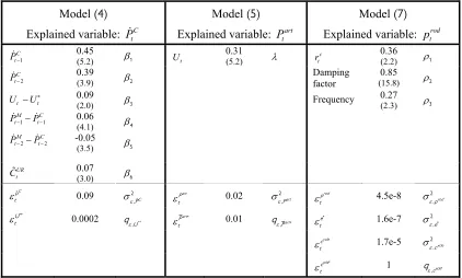
The Kalman filter estimations using the of models (4), (5) and (7) are displayed in Table 1. As in many empirical studies, the signal-to-noise ratio is the only calibrated coefficient. All estimation trials did not give consistent results: they generally lead to a very high value and thus to very volatile TV-coefficients. Labour participation depends on the change in unemployment thus rendering a discouraged-worker effect: a 1 point increase in the unemployment rate would lead to a 0.31 point decrease in the labour participation ratio (Model (5)). Productivity appears to be influenced by the relative cost between labour and capital (Model (7)). If we assume that the share of value added going to profit (α) is 30%, the estimated elasticity of substitution of labour (ρ1) is 36%. This is much lower than the elasticity of the Cobb-Douglas
[image:14.595.83.505.488.742.2]production function (100%). The sharp increase in the relative cost of labour to capital in the 1970’s has led to a growth in labour productivity higher than the growth in technical progress. The disinflationary policy implemented in euro area countries has led to the opposite mechanism from the 1980’s: the slowdown in wage growth and the interest rate hike has led to a lower growth of potential productivity than of the technical progress.
Table 1. Parameters estimates of production function based models
Model (4)
Explained variable: PtC
Model (5)
Explained variable: Ptart
Model (7)
Explained variable: ptrod
1 C t
P− 0.45
(5.2) β1 Ut
0.31
(5.2) λ
c t
r 0.36 (2.2) ρ1
2 C t
P− 0.39
(3.9) β2
Damping factor
0.85
(15.8) ρ2
t t
U −U∗ 0.09
(2.0) β3 Frequency
0.27
(2.3) ρ3
1 1
M C
t t
P− −P− 0.06
(4.1) β4
2 2
M C
t t
P− −P− -0.05
(3.5) β5
UR t
C 0.07
(3.0) β6
εpC
t 0.09 σε2,C
P ε
art
P
t 0.02 σε
2 ,art
P ε
rod
p
t 4.5e-8 σε
2 ,rod
p
εU∗∗
t 0.0002 qε,U** ε
∗
art
P
t 0.01 qε,Part∗ ε
∗
e
t 1.6e-7 σε ∗
2 ,e
ε ycle
c
t 1.7e-5 σε
2 ,ycle
c
ε ycle*
c
t 1 qε,cycle*
For the computation of potential output according to (2), we assume that the population is independent from economic activity which seems a reasonable hypothesis at least for developed countries. Hence, the potential working-age population is working-age population itself and we do not need to apply a HP filter. This is all the more justified that population data are already smooth. The potential labour participation rate and the potential labour productivity are calculated according to Equations (6) and (8).
Because of the additive property of Equation (3), the calculation of the contributions of the unemployment gap, labour participation gap and productivity gap to the output gap is straightforward (Graph 1). According to this model, the output gap would be slightly positive at the end of the sample because productivity would be above the potential. On the contrary, the unemployment and the labour participation gaps would be negative. Moreover, because of the discouraged-worker effect, a share of the labour participation gap may be expressed as a function of the unemployment gap. This share appears to be the most important one since the labour participation gap corrected for the unemployment gap lies always below 0.36%.
Graph 1. Contribution to the Output gap
In % of potential GDP
-4 -3 -2 -1 0 1 2 3 4
1972 1974 1976 1978 1980 1982 1984 1986 1988 1990 1992 1994 1996 1998 2000 2002 2004 2006 Unemployment gap
Productivity gap
Labour participation gap
Source: authors’ calculations.
Graph 2. Contribution to the potential growth
In y-o-y growth rate
-1 0 1 2 3 4 5
1972 1974 1976 1978 1980 1982 1984 1986 1988 1990 1992 1994 1996 1998 2000 2002 2004 2006 NAIRU
Potential productivity
Potential labour participation rate Potential growth Population
Source: authors’ calculations.
3.2. The Multivariate Unobserved Components Model
Formally, all equations in model (9) are estimated simultaneously with the Kalman smoother and the EM algorithm. Innovation variances σεy
2
, ** and σεU**
2
, are
initialised with those of the trends and cycles computed by HP filters. Coefficients of the Phillips and Okun equations are initialised by estimating ordinary equations, where the gap is computed using a HP filter. In order to ease the convergence of the EM algorithm, the variance of Nairu innovations (σεU
2
, **) is constrained to be equal to a
noise-signal ratio (qε, **U ) times the variance of the unemployment gap
(Var Ut Ut σεU γ σεcycle γ
∗
− = 2 + 2 2 − 2
, 6 , 7
( ) /(1 )).
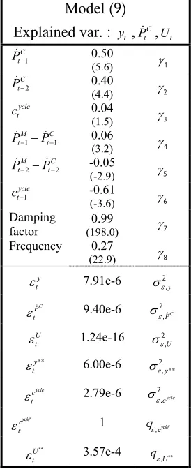
Results of the estimation are displayed in Table 2. The output gap has a frequency equal to 0.27, which corresponds to an average period of 5.8 years. A 1% output gap would imply a positive shock on inflation, equal to 0.04%. Because of the estimated Okun’s law, it corresponds to a negative unemployment gap (-0.61%). However, contrary to the lags of inflation and of the terms of trade, the elasticity of the output gap is not significant at a 5% level, in the inflation equation.
Table 2. Parameters estimates of the MUC model
Model (9)
Explained var. : yt , C t
P ,Ut
1 C t
P− 0.50
(5.6) γ1
2 C t
P− 0.40
(4.4) γ2
ycle t
c 0.04
(1.5) γ3
1 1
M C
t t
P− −P− 0.06
(3.2) γ4
2 2
M C
t t
P− −P− -0.05
(-2.9) γ5
1 ycle t
c− -0.61
(-3.6) γ6
Damping factor
0.99
(198.0) γ7
Frequency 0.27
(22.9) γ8
y t
ε 7.91e-6 σε2y
,
C
P t
ε 9.40e-6
C P ε σ2 , U t ε 1.24e-16 U ε σ2 , y t
ε ** 6.00e-6
y ε σ2 , ** ycle c t
ε 2.79e-6 σεcycle
2 ,
ε ycle*
c
t 1 qε,cycle*
U t
ε ∗∗
3.57e-4
U
qε, ∗∗
Graph 3. Output gap estimate in the MUC model
-4% -3% -2% -1% 0% 1% 2% 3% 4% 5%
1971 1974 1977 1980 1983 1986 1989 1992 1995 1998 2001 2004 2007
Confidence band
around the output gap Output gap In % of GDP
Source: authors’ calculations.
3.3. The Structural Vector Autoregressive Model
In our canonical VAR in three variables (the inflation rate, the logarithm of output and the unemployment rate)
( )
t t t
X = A L X +e (12)
, ,
C t t t t
X = ⎣⎡P y U ⎤⎦ is a vector of non-stationary endogenous variables as output, inflation and the unemployment rate can be considered as I(1) variables. It is then common to use their first difference before estimating the VAR coefficients. Nevertheless, the resulting VAR model in first differences can be written as a VAR model with variables expressed in levels and constraints on some coefficients. When proceeding to estimation of the VAR model in level with no constraints on coefficients, superconvergence of the LS estimators leads to an estimation close to that of the constrained VAR and to residuals of the VAR equations which are I(0) variables. We rely on a well-known principle for an equation including I(1) variables. If the equation is autoregressive with staggered lags and if it is estimated with LS, the estimate will not be spurious. In fact, superconvergence of the LS estimators leads to an equation which can be expressed in terms of I(0) variables. Therefore we choose to work directly with I(1) variables, in order to facilitate output gap calculations.
Table 3. Lag selection criteria
Lag order selection
criteria
Sequentia l modified
LR test
Final predictor
error
Akaike informati
on criterion
Schwarz informati
on criterion
Hannan-Quinn informati
on criterion
Lag exclusion Wald test
Lag order selected by the
criterion
6 6 6 2 2 6
We interpret the results of the Fisher tests of the VAR model, which appear consistent with our priors (Table 4). In the inflation equation, the lags of inflation and of unemployment are globally significant. However, lagged output does not help to explain present inflation. In the output equation, the lags of output and of unemployment are globally significant. However, past unemployment does not explain present output. Finally, in the unemployment equation lags of the three variables are globally significant.
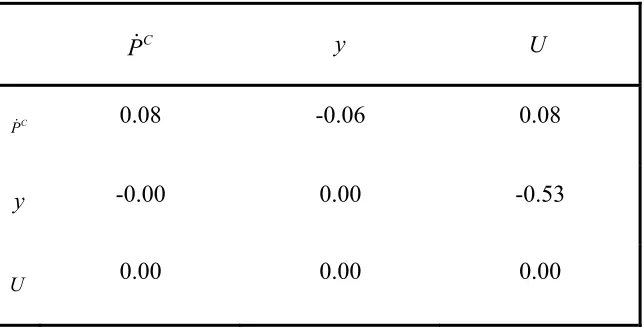
[image:19.595.83.535.426.530.2]Concerning instantaneous correlations of canonical residuals (Table 5), only the one between output and unemployment is significantly different from zero (-0.53).
Table 4. Parameters estimates of the SVAR model – Fisher test
Dependent variable : PC Dependent variable: y Dependent variable: U
F-Statistics
Significance
F-Statistics
Significance
F-Statistics
Significance
C
P 65.29 0.00 PC 6.34 0.00 PC 3.87 0.00
y 0.26 0.93 y 13740.35 0.00 y 6.95 0.00
U 2.39 0.04 U 1.49 0.20 U 4099.07 0.00
Source: authors’ calculations.
Table 5. Covariance-correlation matrix of residuals of the VAR model
C
P y U
C
P 0.08 -0.06 0.08
y -0.00 0.00 -0.53
U 0.00 0.00 0.00
[image:19.595.86.408.580.744.2]Once our SVAR model has been identified (Section 2.3) we rely on the historical decomposition in order to calculate the structural component of output and unemployment.
We use the moving average representation of the structural model (equation 13), where T L
( )
is a matrix of polynomial lags and the vector εt is the one-step ahead forecast errors in Xt given the information on lagged values of Xt:( )
t t
X = +μ T L ε (13)
For a specific date N, the moving average can be expressed as the sum of the forecast for yN+j, based on the information in time N (the term in brackets in equation (14), and of the part based on the time path of the different shocks in the vector of the structural residuals εt, between the dates N+1 and N+j.
Formally, this can be written as:
( )
( )
1
0
j
N j N j k N j k
k k j
X T k ε μ T k ε
− ∞
+ + − + −
= =
⎡ ⎤
= +⎢ + ⎥
⎣ ⎦
∑
∑
(14)In equation (14), the terms in brackets provides the “base projection” of the time series, that is the projection based on the information available at date N (the deterministic and stochastic part up to date N). The first term of the right side of equation (14) contains, for each of the εt, the part of X due to the time path between
N+1 to N+j. This term constitutes the forecast error due to the new structural innovations that hit the system, that is, the part which could not be forecasted at date T and which is the result of structural shocks. In other words, we can attribute the unexpected variation in XT+jto individual structural innovations hitting the economy.
By computing ytas a function of all supply shocks occurring in the time period from the beginning to the end of the sample, we obtain the permanent component of the output in time t. Thus, potential output can be defined as being determined by its deterministic component and by its supply (or permanent) component and obtained as the sum of the “baseline projection” and of the supply shock.
The same calculation is carried out on ut in order to obtain the NAIRU.
According to this model, the output gap (Graph 4) is quite uneven, with five major troughs (1975:2, 1978:1, 1986:1, 1992:4, 1996:1) and shows a positive output gap at the end of the sample. The persistent negative output gap never closes in the nineties until the end of 1999. Ever since effective output exceeds potential output. Peaks coincide with higher than average inflation and troughs with disinflationary episodes. Growth of potential output (Graph 5) is also rather unstable (ranging from -1.2% to 4.2%) and quite close to the effective GDP growth rate.
effective rate of unemployment is lower than the NAIRU since the end of 1999. At the end of the sample the NAIRU reaches 8% of the labour force, while the effective unemployment rate attains 7.3%.
3.3. Comparison of components from different models
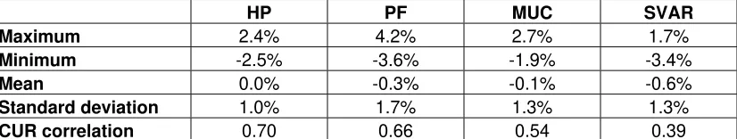
The different methods compared in this paper provide output gap estimates, which are similar in terms of peaks and troughs, but very different in terms of amplitude (Graph 4). The HP output gap shows the lowest amplitudes with standard deviations equal to 1.0 (Table 6). Output gaps obtained with other methods are equal to 1.3.
The SVAR output gap present two peculiarities: contrary to other output gaps, it does not show any positive peak at beginning of the 1990’s and any negative trough at the beginning of the 2000’s. Indeed, since 2001, potential growth of the SVAR model is very close to effective growth, while other models provide quite stable potential growth rates (around 2%, see Graph 5). Finally, the SVAR output gap has the lowest correlation with the capacity utilization rate (0.39, Table 7) and this illustrates the difficulty for interpreting the evolution of such a gap.
The MUC model gives the smoothest output gap estimate (Graph 4) whereas the smoothest estimate of the potential growth is provided by the PF approach and the HP filter (Graph 5). Nevertheless, the PF estimate of the potential growth seems more satisfactory that the HP one because it is less cyclical. The cyclicality of the HP estimate is not surprising since it provides the GDP trend and not a real estimate of the potential output. All of the NAIRU estimates show a global decline since the mid-1990’s, but the NAIRUs of the MUC and PF models are smoother than those of other models (Graph 6). This outcome is quite predictable since the specifications of the Phillips curve in both models are quite similar. Moreover, the MUC model provides the lowest NAIRU at the end of the sample (6.9% in 2007:1). In 2007:1, the highest estimate (8%) is provided by the SVAR model and it is higher than the effective unemployment rate (7.3%).
[image:21.595.91.504.538.616.2].
Table 6. Descriptive statistics
HP PF MUC SVAR
Maximum 2.4% 4.2% 2.7% 1.7%
Minimum -2.5% -3.6% -1.9% -3.4%
Mean 0.0% -0.3% -0.1% -0.6%
Standard deviation 1.0% 1.7% 1.3% 1.3%
CUR correlation 0.70 0.66 0.54 0.39
Legend: HP = Hodrick-Prescott filter; PF = production function based model; MUC = multivariate unobserved components models; SVAR = structural VAR model. CUR correlation: correlation of output gaps with capacity utilization rate.
Graph 4. Output gap of the euro area, estimated with various methods
-4 -3 -2 -1 0 1 2 3 4 5
1970 1973 1976 1979 1982 1985 1988 1991 1994 1997 2000 2003 2006
HP PF M-UC SVAR
In % of potential output
Legend: HP = Hodrick-Prescott filter; PF = production function based model; MUC = multivariate unobserved components models; SVAR = structural VAR model.
Source: authors’ calculations.
Graph 5. Potential growth with various methods
-3 -2 -1 0 1 2 3 4 5 6 7
1972 1975 1978 1981 1984 1987 1990 1993 1996 1999 2002 2005
HP PF M-UC SVAR Effective growth
In y-o-y growth rates
Legend: HP = Hodrick-Prescott filter; PF = production function based model; MUC = multivariate unobserved components models; SVAR = structural VAR model.
Graph 6. NAIRU with various methods
0 2 4 6 8 10 12
1972 1975 1978 1981 1984 1987 1990 1993 1996 1999 2002 2005
HP PF M-UC SVAR Unemployment rate In % of the labour force
Legend: HP = Hodrick-Prescott filter; PF = production function based model; MUC = multivariate unobserved components models; SVAR = structural VAR model.
Source: authors’ calculations.
3.4. Comparing turning points from different models
The turning points of each output gap estimate are computed with the standard Bry-Boschan algorithm. For each output gap xi,t , a chronology Si,t is deduced, which
takes the unit value in the case of an expansion and a zero value in the case of a slowdown. Then, each chronology Si,t is characterized by two basic statistics, the
averaged duration of expansions and of slowdowns. It is also compared to the reference chronology Rt of Anas et al. (2008, see table 2, p. 10), which has two main
advantages:
• this is a growth cycle chronology like ours;
• this chronology has been built with the NBER 3D’s philosophy (deepness, duration, diffusion) implemented through the algorithm of Harding and Pagan (2002).
Moreover, this chronology could become a reference one, as Eurostat is currently assessing it. The comparison of each chronologies Si,t with the reference chronology
Rt is performed through the concordance statistic:
(
) (
)
(
)
1
, ,
1
1 1
T
i i t t i t t
t
C T− S R S R
=
⎡ ⎤
=
∑
⎣ ⋅ + − − ⎦.Table 7. Comparison of growth cycle chronologies
REF HP PF MUC SVAR
Expansion duration 9.3 8.0 8.9 14.2 6.6
Slowdown duration 5.5 6.2 7.1 11.4 8.3
Concordance 1.00 0.78 0.76 0.63 0.48
Legend: REF = reference chronology of Anas et al. (2008); HP = Hodrick-Prescott filter; PF = production function based model; MUC = multivariate unobserved components models; SVAR = structural VAR model. Averaged durations of expansions and slowdowns are measured in quarters. Concordance: concordance of expansion/slowdown chronologies dated with each output gap and with the reference chronology.
Source: authors’ calculations.
3.5. Comparison of inflation forecasts from different models
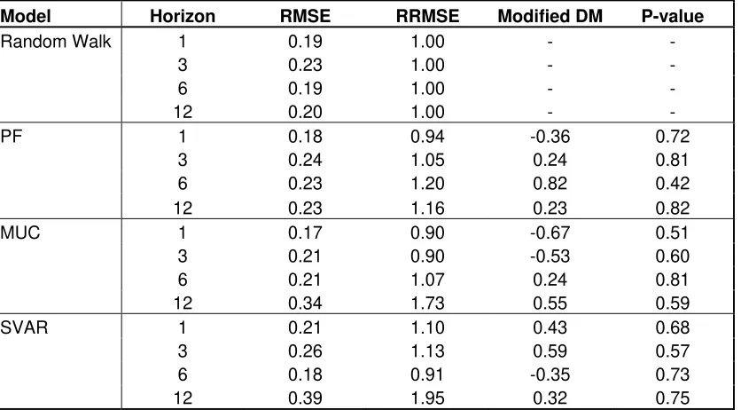
The different models are compared according to their ability to forecast inflation (Table 8). The naive model, specified as a random walk model, is used as a benchmark. The modified Diebold-Mariano statistic is used in order to test if a model is statistically better than the naive model for out-of-sample forecasts of inflation (see Harvey, Leybourne and Newbold, 1997, for details about this test). The MUC model is better than the naive model for short run horizon (RRMSE<1 for horizons 1 and 2), but this advantage is not statistically significant according to the modified Diebold-Mariano test. The SVAR model is better than the random walk model for medium run horizon (RRMSE<1 for horizon 6) but this advantage is not significant either. The PF model performs worse than the naive model except for the shortest horizon (RRMSE>1).
Table 8. Inflation forecast with various methods
Model Horizon RMSE RRMSE Modified DM P-value
Random Walk 1 0.19 1.00 - -
3 0.23 1.00 - -
6 0.19 1.00 - -
12 0.20 1.00 - -
PF 1 0.18 0.94 -0.36 0.72
3 0.24 1.05 0.24 0.81 6 0.23 1.20 0.82 0.42 12 0.23 1.16 0.23 0.82
MUC 1 0.17 0.90 -0.67 0.51
3 0.21 0.90 -0.53 0.60 6 0.21 1.07 0.24 0.81 12 0.34 1.73 0.55 0.59
SVAR 1 0.21 1.10 0.43 0.68
3 0.26 1.13 0.59 0.57 6 0.18 0.91 -0.35 0.73 12 0.39 1.95 0.32 0.75
Legend: RMSE (root mean squared errors); RRMSE : ratio between the RMSE of the model tested to the RMSE of the naive model (Random walk); Modified DM : modified Diebold-Mariano statistic; p-value associated the absolute p-value of the modified DM statistics.
[image:24.595.90.508.480.711.2]4. Real time estimation
The empirical comparison focuses now on the real-time properties of the PF, MUC and SVAR models. The HP filter is used as a benchmark. Estimates and revisions of output gaps are also computed with various horizons. For each method, two estimates of output gaps are compared:
• real-time estimates of output gaps at the date t are estimated with the sample
[1970:1 ; t], which is available at the first publication of all required variables at the date t;
• quasi real-time estimates of output gaps at the date t with an horizon h are
estimated with the revised sample [1970:1 ; t], which is available h months after the first publication of all required variables at the date t;
• revised estimates of output gaps at the date t with an horizon h are estimated
with the sample [1970:1 ; t+h/4], which is available h months after the first publication of all required variables at the date t;
with t = 2000:3, …, 2007:1, h = 1, 3, 6, 12, 24 or 36 months and q = 0, 1, 2 ,4, 8, 12 quarters the horizon expressed in quarters. Then, for the horizon h, the real time
revisions of output gaps are the differences between the revised estimates of output
gaps and their real-time estimates. The data revisions correspond to the differences between the quasi real-time estimates of output gaps and their real-time ones. The
quasi-real time revisions are computed as the difference between the quasi real-time
and the revised estimates. The root mean squared errors (RMSE) of all those revisions are presented in Table 9.
In the case of the HP filter, the general result shown by Orphanides and Van Norden (2002), shown for the main univariate methods, is confirmed for all horizons. The impact of data revisions (RMSE between 0.05 and 0.12 for h between 1 and 36 months) is low compared to real-time revisions (RMSE between 0.11 and 1.03 for h between 1 and 36 months). Moreover, the data revisions of the HP filter are lower than those of other methods. This reflects the famous end of the sample bias of the HP filter where new data often modify the last HP estimate.
The stability of multivariate estimates, shown with quasi real-time estimates by Camba-Mendez and Rodriguez-Palenzuela (2003), is confirmed with a real-time dataset. For a sufficiently long horizon, e.g. 12 months, the RMSE of the HP filter in real-time (0.60) is higher than those of multivariate methods (0.51 for the MUC approach and 0.33 for the SVAR model). For short horizons, e.g. 1 or 3 months, the real-time revisions are not worse with the HP filter (RMSE equal to 0.11 for h = 1) than with multivariate methods (0.12 for the MUC approach and 0.14 for the SVAR model). Because of its autoregressive structure with long lags, the SVAR model implies the lowest revision with a relatively stable RMSE across time horizon.
of the HP filter and of the MUC model for the longest horizon (RMSE of 0.55 for h = 36 months).
Table 9. Comparison of output gap revisions
Horizon Revision type HP PF MUC SVAR
1 month Real-time 0.11 0.39 0.12 0.14 Data revision 0.05 0.15 0.09 0.09 3 months Real-time 0.19 0.61 0.17 0.23 Data revision 0.08 0.21 0.13 0.14 6 months Real-time 0.34 0.79 0.28 0.32 Data revision 0.10 0.27 0.13 0.19 12 months Real-time 0.60 0.75 0.51 0.33 Data revision 0.12 0.34 0.15 0.23 24 month Real-time 0.89 0.61 0.76 0.40 Data revision 0.12 0.34 0.17 0.31 36 months Real-time 1.03 0.55 0.84 0.51 Data revision 0.12 0.29 0.16 0.38
Legend: The real-time revisions of the output gap (type “Real-time”) and the impact on it of data revisions (type “Data revision”) are computed for each method and various time horizons by the root mean squared error (RMSE). HP = Hodrick-Prescott filter; PF = production function based model; MUC = multivariate unobserved components models; SVAR = structural vector auto-regressive model.
Source: authors’ calculations.
5. Ranking and concluding remarks
This paper has explored the forecasting power and real-time properties of different approaches used for estimating potential output. This empirical achievement has been obtained by improving the theoretical framework of the production function approach, before its comparison with the multivariate unobserved components (MUC) approach and with the structural vector auto-regressive (SVAR) approach. The main conclusion is that the different estimation methods of the potential output have all advantages and drawbacks. The choice of the estimation strategy depends on the specific needs of the final user of output gap estimates.
in this paper does not rely on the imprecise series of the capital stock. As other multivariate methods (MUC and SVAR), the PF approach has better real-time properties than the univariate HP filter. Indeed, the HP estimate is largely revised like all univariate methods (see Orphanides and Van Norden, 2002). However, real-time analysis could be completed by uncertainty criteria, which we would like to implement in future research.
Appendix A. The production function approach
Our PF model consists in 3 estimated economic behaviours: (1) a reduced Phillips curve in order to estimated the NAIRU, (2) a labour participation equation and (3) a productivity equation. In this Appendix, we give the theoretical background of each relation.
A.1. Phillips curve and NAIRU
There are mainly two estimation methods of the NAIRU (or equilibrium rate of unemployment). The structural approach follows a two-stage procedure. First, a structural model of wage and price equations is estimated. As the NAIRU is the unemployment rate that stabilises inflation, it can then be calculated as a function of the estimated parameters and of the variables of the structural model (see Chagny, Reynès and Sterdyniak, 2002, or Heyer, Reynès and Sterdyniak, 2007). The popular Time-Varying (TV) NAIRU reduced approach inspired by the Gordon (1997) triangle model has only one step. The NAIRU is estimated simultaneously with a reduced Phillips curve using the Kalman filter. The Gordon (1997) triangle model states that inflation depends on past inflation (adaptative expectation), the unemployment gap,
i.e. the gap between the unemployment rate and the NAIRU ( *
U ) and temporary supply shocks:
*
1 ( )
S
P=γP− −β U−U +μS +ε (13) where P is the price level, S
S the supply shocks and ε a white noise.
It can be shown how this model can be deduced from a structural model of wage and price equations (Heyer, Reynès and Sterdyniak, 2007). Most of the time, a full indexation on the past inflation is assumed (γ = 1) so that the NAIRU is independent of inflation because of the absence of trade-off between unemployment and inflation.
The latter equation is estimated simultaneously with the one of *
U which may be a purely stochastic process or also depend on observable variables suggested by economic theory (the unemployment rate in case of hysteresis5, labour productivity, the interest rate, the minimum wage level, trade union membership, the unemployment benefit replacement rate). Thus a general specification is:
1 . 1 .
t t t t t
U∗=U∗− + Δϕ U− + +ρ δ X +ε′ (14) where ϕis a constant, ρ a trend, X a set of exogenous variables and ε′ a white noise.
In the literature, the specification is generally a particular case of Equation (14). Following Gordon (1997) and King et al. (1995), the long-term ERU (ERULT) is often
specified as a random walk (Equation (15) in Table A.1). Since the random walk hypothesis often gives disappointing results in both cases of France and Europe (see Irac, 2000; Richardson et al., 2000; Laubach, 2001), the econometric properties of the model may be improved in three ways simultaneously. The first is by testing other ad hoc stochastic specifications of the NAIRU, for instance by adding a stochastic trend (e.g. Equations (16) and (17) in Table A.1). The second is by trying to find observable determinants of the NAIRU (Equations (18) to (21) in Table A.1). The third approach used to improve the model entails adding other equations in which the NAIRU is assumed to have an influence. While some such additional equations, such an Okun’s law (Equation (24) in Table A.1), have an economic interpretation, others are rather
5
ad hoc. For instance, Equations (22) and (23) impose that the unemployment gap is stationary.
Table A.1. Some specifications of the TV-NAIRU in the literature
Constrained version of (14) Authors
(15) Ut*=Ut*−1+εtU* Gordon (1997) / King et al. (1995)
Irac (2000) drops the hypothesis of
white noise: 1
LT LT
U U
t t t
ε =θε− +ε′
(16) * * *
1 .
χ′ − ε
Δ = Δ + U
t t t
U U Richardson et al. (2000)
(17) * = *−1+ρ ε+ *
U
t t t t
U U with t t 1 t
ρ
ρ =ρ− +ε Laubach (2001)
Fabiani and Mestre (2001) Denis et al. (2002)
(18) * * *
1 α 1 ε
− −
= + + U
t t t t
U U U Jaeger and Parkinson (1994)
(19) Ut*= +ϕ ρ γt+ .Xt+εUt* with ρt =ρ′.t
X :real interest rate, tax wedge, trend growth rate of the GDP
Mc Morrow and Roeger (2000)
(20) Ut*=Ut*−1+γ.X +εtU*
X : variations in the unemployment rate, the long-term interest rate and in the labour productivity growth, the ratio between the minimum wage and the average wage
Heyer and Timbeau (2002)
(21) *= *−1+ρ γ+ . +εU*
t t t t
U U X with ρt =ρt−1+εtρ
X :variations in the short-term interest rate and in the labour productivity growth
Logeay and Tober (2003)
Additional equations Authors
(22) Ut−Ut*=ν(Ut−1−Ut*−1)+εt Apel and Jansson (1999)
Laubach (2001)
Fabiani and Mestre (2001) Denis et al. (2002)
(23) ΔUt = Δν Ut−1−ν′(Ut−1−Ut*−1)+ν′′X+εt X :variation in inflation
Heyer and Timbeau (2002)
(24) yt−yt*= −ν(Ut−Ut*)+εt with yt*= +ν′ yt*−1+εty*
Y and Y* are the effective and potential outputs.
Apel and Jansson (1999) Laubach (2001)
Fabiani and Mestre (2001)