The automatic design of experiments : Some practical
algorithms.
GREENFIELD, A. A.
Available from Sheffield Hallam University Research Archive (SHURA) at:
http://shura.shu.ac.uk/19724/
This document is the author deposited version. You are advised to consult the
publisher's version if you wish to cite from it.
Published version
GREENFIELD, A. A. (1979). The automatic design of experiments : Some practical
algorithms. Doctoral, Sheffield Hallam University (United Kingdom)..
Copyright and re-use policy
See http://shura.shu.ac.uk/information.html
PuND S IR FFI I SHEFFIELD SI IVVB J
ProQuest Number: 10697026
All rights reserved
INFORMATION TO ALL USERS
The quality of this reproduction is dependent upon the quality of the copy submitted.
In the unlikely event that the author did not send a com plete manuscript and there are missing pages, these will be noted. Also, if material had to be removed,
a note will indicate the deletion.
uest
ProQuest 10697026
Published by ProQuest LLC(2017). Copyright of the Dissertation is held by the Author.
All rights reserved.
This work is protected against unauthorized copying under Title 17, United States C ode Microform Edition © ProQuest LLC.
ProQuest LLC.
789 East Eisenhower Parkway P.O. Box 1346
The Automatic Design of Experiments
Some Practical Algorithms
by A. A. Greenfield B.Sc., F.I.S., F.S.S.
A thesis submitted to the Council for National Academic Awards for the degree of Doctor of
Philosophy
The Automatic Design of Experiments
Some Practical Algorithms
ABSTRACT
The purpose of this study was to develop a methodology, represented as a set of programmable algorithms, for the design of experiments of the types that are generally likely to be useful in the physical sciences. This has been achieved by adding to the established theory and practice of designing factorial experiments for both qualitative and quantitative variables.
Algorithms were developed for designing fractional two-level factorial experiments according to a pre-specified model to be fitted, expressed in terms of required effects to be estimated. These algorithms are extended in two ways. One of these is to allow a fractional two-level factorial design to be augmented with extra points so that quadratic effects can be estimated. The second is to enable fractional asymmetric multi-level factorial experiments to be designed: balanced fractions first by applying the theory of cyclic groups; then further reduction in the size of the design by using the trace and determinant of the information matrix.
The application of the algorithms is illustrated with examples drawn from the physical sciences, particularly metallurgy.
The algorithms developed in the study have been fully implemented using standard Fortran 4 with a few specified exceptions. These programs are listed in three appendices. The programs have been run on computers in research laboratories in Australia' and . the United States as well as in Britain. They will benefit research scientists who are planning experiments and have access to interactive computers.
The Automatic Design of Experiments
Some Practical Algorithms
CONTENTS
Chapter one INTRODUCTION
1 Background 2 Objectives 3 Algorithms
Chapter two CHOICE OF EXPERIMENTAL CLASSES
Chapter three TWO-LEVEL FACTORIALS 1 Background 2 Algorithms 3 Examples
Chapter four QUADRATIC DESIONS 1 Background 2 Algorithms 3 Examples
Chapter five ANALYSIS AND SIMULATION 1 Introduction 2 Examples
Chapter six FRACTIONAL ASYMMETRIC MULTI-LEVEL FACTORIALS
Chapter seven
Chapter eight
Appendices
REDUCING THE BALANCED ASYMMETRIC FRACTION
1 Background 2 Using the trace 3 D-optimal algorithms 4 Examples
3 References
CONCLUSIONS
1 Work done 2 Further work 3 Acknowledgements
REFERENCES
CLOSSARY
APPENDIX ONE
Programmed algorithms of chapters three and four
APPENDIX TWO
Programmed algorithms of chapter six
APPENDIX THREE
CHAPTER
The Automatic Design of Experiments
Some Practical Algorithms
ONE
INTRODUCTION
1 Background
2 Objectives
1 Background
Gauss (1809) was the first person to allude to the design considerations of making physical observations. Most of his great work on the theory of the motions of
heavenly bodies was devoted to the development of algorithms for computing orbits from precise observations. Then,, in the third section of the second book of the work, he developed the normal, or Gaussian, density function and the method of maximum likelihood, and he presented the method of least squares (which he claimed to have been using since 1793) aril the method of weighted least squares. In the midst of this he commented, as an aside and without proof, that if only a few observations were to be made to determine an orbit they should be as remote from each other as possible to minimise the effects of observational errors. When he later developed
this statistical theory into a full treatise (1821) he discussed at some length the further design problem of the effect of an extra observation on already estimated coefficients and the conditions that must be imposed to ensure minimum variance of jfahe estimates.
It was a century later when Smith (1918) suggested' maximising the determinant of X'X, known as the information matrix or the cross-product of the design matrix (X), as a criterion for designing experiments. The determinant is inversely proportional to the generalised variance of the estimated coefficients. Smith applied her criterion to experiments for estimating polynomials of varying
interval over which the polynomial should be fitted, she determined the spacings between observation points and the proportions of observations to be made at those points in order to minimise the generalised variance of the
estimates of the coefficients of the polynomial. The method is neatly presented in three pages by Kendal and Stuart (1966) who had the advantage over Smith of modern matrix notation and algebra. However, despite the clumsy notation of her day, Smith went on to consider the effect of heteroscedasticity of errors on the optimum allocation of observations.
The concept of experimental design grew most rapidly in agricultural work. Fisher (1923) introduced the subject briefly in his first edition of ’Statistical Methods for
Research Workers.' He illustrated that applied statisticians were mainly concerned with data examination, analysis, and statistical tests of conirasts. The method of experimental design seems to have been: think of an arrangement of
trials, such as a Latin square, then see if the arrangement meets the experimental criteria. These criteria were: can the desired contrasts be estimated from the data, and will the arrangement lead to statistical tests of the estimated contrasts?
It seems as if Fisher realised the importance of experimental design at the time the book was published, for within a year (1926) he published a major paper on 'The arrangement of field experiments' and later wrote the first definitive text (1933) on 'The design of experiments'.
Fisher had a profound effect on the development of
qualitative factors or could be treated as such, and the method of analysis was 'analysis of variance'. He and his contemporaries applied considerable ingenuity to finding designs which were orthogonal in that the contrasts between levels of different factors could be estimated
independently. A host of design types was developed: randomised blocks, balanced incomplete blocks, split plots, Latin squares, Youden squares, anr< lattices, among the better known. Many books were written about these agricultural designs, variations on them, applications, their analysis, and what to do when missing values upset the balance and made estimation and testing difficult. The most authoritative of the books covering the subject were probably Cochran and Cox (1950), Kempthorne (1952), Brownlee (1953)> and Davies (1954)* Uses were found for these designs in other than the agricultural sciences. They were applied with quantitative variables as well as qualitative: the levels of the quantitative factors were usually equally spaced for convenience. The criterion proposed by Smith in 1918 seemed to have passed unnoticed.
theoretical unification of the methods of analysing these types of design was presented by Tocher (l952cj) when h'- at the same time suggested that, computers be set to work to generate all possibly useful designs. There were several warnings in the discussion of that paper against the 'sausage machine' approach to experimental design.
Tn his 1926 paper, Fisher discussed the concept of
general discussion at Rotfaaasted. Fisher argued that while these could become very large and complex experiments, they had the advantages that:
1 the plots are used several times over to determine the average effects of different factors;
2 only by factorial design can any information be obtained on how responses to one factor are affected by another (that is: they permit the estimation of interactions);
3 factorial experiments provide a wider inductive basis for conclusions on the effects of the factors;
At the same time he recognised the possibility of
confounding: the deliberate sacrifice of some unimportant information so as to improve the precision of estimates of important effects. The methodology for dealing with confounding was developed by Yates (1933) who also designed an algorithm (1937) for easy analysis of
two-level factorials. A further advantage of confounding was soon realised: it could be used to select a fraction of a factorial. The theory of fractional replication was developed by Finney (1945) and Kempthorne (1947)»
The development of agricultural type experiments by the Fisher group was represented in so much literature that for several decades the rest of the scientific world was largely misled into believing that the subject of
experimental design comprised an understanding of only those agricultural designs. Also, because the mean effects or contrasts were so easy to compute, estimation was largely disregarded as an aspect of
analysis and the emphasis was placed on tests of significance In'The Design of Experiments' Fisher wrote: 'Every
experiment may be said to exist only in order to give the facts a chance of disproving the null hypothesis,'
Experimentation in the physical sciences is often much more complicated than the traditional field trials, and estimation of effects is not so easy. Thus analysis tends to be by the regression method of least squares as developed by Gauss rather than by Fisher's analysis of variance. It was Tocher (1952a) who showed that
regression analysis was applicable to designed experiments as well as to naturally occurring data. This observation, together with a growing literature on determining the
the Kieffer school (see. Kieffer and Wolfovitz (1959)* Kieffer (1959), Wynn (1970, 1972)) are long, intricate, mathematically involved, and literally obscure, so that they have had little influence on the originally applied subject of experimental design. Indeed the subject has gone two ways: at the applied level there have been some developments of agricultural type experiments, particularly in the augmentation of two-level factorials with extra points to permit the estimation of quadratic effects (which will be described in chapter four); and on the theoretical level it has become a branch of
2 Onjectives
One of the objectives of the present research has been to make a practical contribution which will help non- statistical research scientists, particularly physical scientists such as chemists, physicists, metallurgists, and engineers, with a fairly closely defined sub-area of what has become a massive subject. Just as there has had to he some selection of material for the
preceding historical introduction, with many aspects omitted and many contributors unmentioned, the choice of a sub-area that can reasonably be tackled in a single study must inevitably leave most of the
subject untouched.
The choice will be discussed more fully in chapter two. ■ t. this stage let it suffice that the aim has been to meet most of the experimental design needs of
physical research and to develop automatic methods of design that will obviate the need for the research worker 1f' identify the type of design suitable for his work. ''’he interactive nature of the algorithms that have been developed will lead naturally, through questions and
A classical research situation, encountered almost daily in any industrial laboratory for research and development, can be described as follows:
The objective is first declared as the optimisation of a product or a process; the characteristics of that product are identified; precisions of measures of those characteristics are stated; and the control variables are identified, usually the compositional and process variables, with ranges and precisions.
Sometimes the objectives of the experiment are represented as a mathematical model relating the measures of the product characteristics with the control variables, but this is rare. More usually the
research worker has little idea of the pertaining relationships and can express them only in vague qualitative terms. Clarity usually follows questioning, however, so that it is possible to write down at least a simple linear model including expected first order interactions and perhaps also to include some quadratic terms.
On the basis of this information an experiment is designed so as to estimate the parameters of the model as precisely and as accurately as possible within the limitations of experimental costs. The objectives of an experiment must always be to answer a precisely stated question or set of questions. Almost always these questions can be stated in terms of a mathematical model whose parameters are to be estimated or perhaps compared with an alternative model. Sometimes an objective goes so far as to include optimisation, but even this is a particular case of estimation.
labour was probably worthwhile■because a suitable fraction Would achieve the experimental objectives with considerable cost and time savings. It was the original purpose of this study to assist the research worker in obtaining quickly and easily an experimental design suitable to his objectives. The aim was for the following
dialogue to take place between the laboratory computer and the research metallurgist. The dialogue would be through a keyboard and typewriter terminal.
The user would first establish the date and research name, where upon the program would open up a new data file under that name. It
would then begin to ask the user questions about his variables. Which . are the dependent variables and which are the independent? The answers may be given as names or as numbers. Also identified would be the intermediate variables which, to the physical metallurgist say, may be worth recording to extend his fundamental understanding of the subject, but from the viewpoint of a predictive statistical model may be
ignored. An example of this type of variable is grain size. It is not an independent variable from the viewpoint of experimental design because it cannot be controlled directly. Strictly it is a dependent variable because grain size is determined as the response to control or independent variables such as composition and process treatment. On the other hand it cannot be claimed to be a commercial characteristic of steel, although there are said to be relationships between the grain size and the
commercial characteristics. So I call it an intermediate variable.
Figure 1 x »
The computer program would allocate a disk area to the research project and would store the information so far obtained. It would then produce the most efficient design corresponding to this information.
The research worker would be expected to follow the computer-printed design and return to the computer later with his results. The analysis programs would take into account any missing, spoilt, or extra data. The computer would produce reports in the form of prints of the analysis, plots of contours, and sections of response surfaces. These would assist the user to determine whether to make further observa tions, in which case the computer would offer its advice on further
observation points, or to produce a final report and clear the disk area for another user.
Process research increasingly calls for the real-ti»e analysis of data as it is collected, rather than waiting for an experiment or a series of experiments to be completed before data analysis begins. This presents the further challenge of automatic sequential analysis of data and synchronous revision of experimental design. Thus the aim of this research included, originally, the prospect of extending to the on-line situation the automatic design and analysis of experiments already described. In these cases we should be logging data from and controlling processes whose properties may not be known in advance: the computer would establish mathematical models describing the processes and would improve these models as it acquired more data. Thus the computer would learn from experience, but rather more quickly than a human being, although admittedly with some limitations.
and keyboard connected directly to the central computer. Terminals would be labelled with types of signals that could be connected: analog input and output, digital input and output; and the permitted voltage ranges. Within the computer would be a suite of generalised data analysis, acquisition, and control programs. The user in the laboratory would connect leads from his experimental process to the termination board. Through his keyboard he would have a conversation with the computer similar to that described for the off-line automatic design and analysis of experiments. He would signal to the computer when the experiment was set up and ready to go. And it would go! The flexibility must be stressed: it would not matter to the system whether the experimental process under study was a miniature electro slag refining plant or a tomato plant, so long as the signal types, voltage ranges, and sampling frequencies were suitable to the computer.
In some ways the original aim of this research as described
above was over-ambitious and unrealistic. Within limitations, however, it is still practical and achievable, certainly worth pursuing, and some of it is already within reach.
One of these limitations is dictated by the plethora of approaches to experimental design. The review paper by Herzberg and Cox
listed nearly 900 references. It is notable that most were of a highly theoretical and non-applied nature and rone was concerned with automatic design of experiments as an aid to the industrial research scientist. That paper nevertheless highlighted a point of considerable importance in this current study: that the class or classes of experiment studied should be sufficiently narrow to allow significantly noticeable and useful progress. This point was made by Tocher(t^S2§who wrote: "It soon became clear that any such account, if treated in the detail commensurate with the importance of the subject, would be excessively long and that some curtailment of the programme would be necessary. Consequently, ... attention is concentrated almost entirely on those experiments normally referred to as block experiments."
A further limitation is the extent to which a conversation between research worker and computer can be allowed to proceed without the guidance of a statistician* While it should be possible to develop programs to support question a nd answer routines with descriptive text and graphical illustrations to explain difficult points to the conversing scientist, when he seeks clarification, it became
apparent during the study that such a system would be far from easy to implement* Indeed, to be wholly satisfactory, it would need a much deeper study into the psychology and linguistics of program instruction* Hence, while the original aim of developing automatic design procedures was maintained, it has been restricted to
providing an aid to the applied consulting statistician and to the initiated research scientist rather than providing a conversational system available to all-comers regardless of their knowledge, or lack of knowledge, of elementary mathematical modelling and experimental design and analysis.
3 Algorithms
In publications related to the earlier stages of this research (Greenfield (1972,1974)) the procedures that were developed were illustrated in program segments written in an extension of standard Fortran 4. The full programs were published as appendices. These programs were freely available and research laboratories in several countries tried to Implement them. Some were successful and some were not* The problem was that programs are in general not easily portable from one machine to another even if the machines are claimed to support the same high level language because differences between machines lead to a unique dialect of a high level language for each. If a program were written precisely in Fortran 4 it would be portable. However, dialects are sufficiently different that an•implementer may not see how to convert a program. Some dialects have extensions that are oriented towards toe class of applications for which <the computer has been designed. This applies particularly to scientific computers. It may he argued that programmers should stick rigidly to th*' standard, but if they do not use all the available extensions they are underusing the facilities.
clearest way to describe a complicated procedure. On the other hand, a sequence of steps in English is not.
adequate to describe other than the simplest of mathematical procedures. In this thesis, therefore, an algorithmic style, which has recently become conventional in the computing world, will be used. This has advantages that will be described below.
An algorithm is a sequence of rules for solving a problem, usually, but not always, mathematical. The word is not new. It has been used with this meaning in English, German, and Latin (algorismus) for some centuries. Much of Gauss's astronomical and statistical work was couched in algorithmic terms and he used the word in the modern sense. However, in recent years it has become clear in computing circles that communication would be greatly improved if a universal convention for stating algorithms were adopted.
A secondary purpose of an algorithm is to supply a sequence of rules that will minimise the time and effort needed to reach the correct solution to the problem for any arbitrary initial values.
Another purpose of an algorithm, and one that h»s become increasingly important, is to provide a*
sequence of rules that are easy to understand, simple to prove correct, and easy to change if the specifications of the problem and the way to solve it change. As
algorithms become more and more complex there is increasing difficulty in understanding how they work, how to find and correct errors, and how to make development changes. It. has been claimed that more than half a programmer's time is spent dealing
with program correction, maintenance, and modification. Leading programmers, most notably Dijkstra (1973),
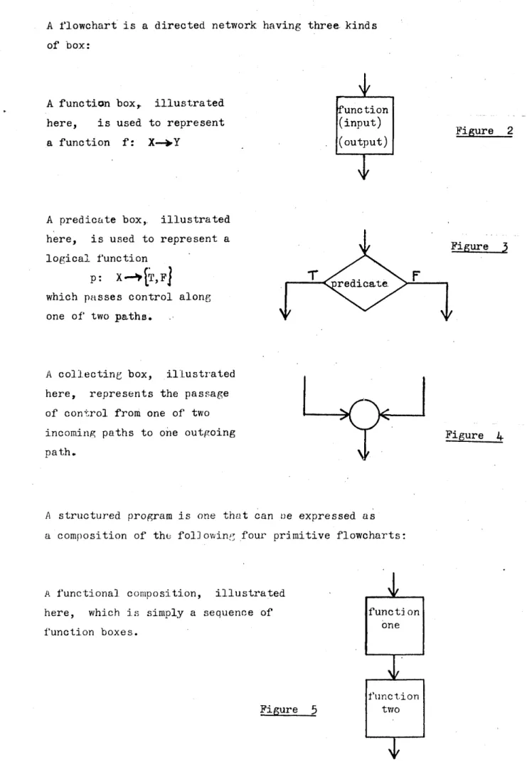
A flowchart is a directed network having three, kinds of box:
A function box,, illustrated here, is used to represent a function f: X—
function (input)
(output) Figure 2
A predicate box,, illustrated here, is used to represent a logical function
p: X — *[t,f|
which passes control along one of two paths.
Figure 5
redicate
A collecting box, illustrated here, represents the passage of control from one of two incoming paths to one outgoing
path.
O
V
Figure U
A structured program is one that can ue expressed as a composition of the fol]owing four primitive flowcharts:
A functional composition, illustrated here, which is simply a sequence of function boxes.
functi on one
A selection, illustrated here,, which uses a logical test, whose outcome is either true or false* to determine which of two alternative functions should be done. In practice, a test with more than two outcomes may be used but this is equivalent to a sequence of two-outcome tests.
Two forms of iteration in which a logical test is used to decide whether or not a function should be repeated. The distinction between the two.forms is that in one the first time the test is met is before the f irst time the function is met, and in the other the order of the first meeting is reversed.
Figure 6
predicate
function two
function
one
functDon
Figure
function
predicate
thms in terms 01. structured flowcharts. Top-down structured programming means starting with a general statement of a function and then analysing it a step at a time into levels of greater detail until the stage is reached when code can be written easily in a high level language to implement the developed algorithm. This final stage is best done in certain languages like Algol and Coral which have been designed with an algorithmic nature. It is much more difficult, although still possible, with Fortran which has
a different structure. I shall however use Fortran to illustrate programming features because it is by far the
ScJe^KKc
most widely used^programming language.
The topr-down structured programming procedure will be illustrated with reference to Euclid's algorithm for
determining the highest common, factor (hcf) of two integers.
This is also known in America as the greatest common divisor (gcd). I have chosen Euclid's algorithm as an
illustration for three reasons: it is needed as a sub routine in the experimental design algorithms developed in chapter six; it is complex enough to illustrate development at several levels of detail; it is short enough and simple enough to serve as an illustration.
At the same time as using the example to illustrate top down programming in terms of flow chart representation, I
Shall use the occasion to illustrate the conventional linguistic representation. This bears a striking resemblance to the programming language Algol, an apt neologue from 'algorithmic language'. The conventions used for describing algorithms are however much more flexible than those of a programming language which has
strict rules rather than useful conventions. Thus an algorithmic step may be described in the broadest functional terms using English or mathematical notation, rather than in explicit computational expressions, assignments and tests, although at the final stage of developing an algorithm these latter will appear.
underscore. Examples are: algorithm, and, do, else,r ^ AAA/ 7 A^»7 7 fi, for> goto, if, od, set, then, through, to, while. An algorithm name is set in holdface capitals, such as HCF. The derivation of an algorithm name may be italicised in parentheses* In typed copy italics are indicated by a straight underscore. For example:
Algorithm I1CF (Highest Common Factor)
The word 'step' followed by a number, is used to label a step in the algorithm and is also set in italics: Step 5
This label may be indented to indicate the level of logic.
Immediately after the label Step i, a brief phrase in roman medium typeface in square brackets to describe the purpose of the step. Further comments, also in roman medium type, may appear within the step and are usually separated by semi-colons.
Mathematical, logical, and computational expressions are also put in medium type. The reverse arrow is used for assignment. For example:
means that the variable K is assigned the value
1.20
In top down structured programming we repeatedly ask if the function being considered can be expressed as
a primitive flowchart. Top down programming is illustrated in the following example which starts with a single function box. In practice* I do not always use strictly structured programming because it sometimes seems clumsy.
Algorithm HCF (Highest Common Factor)
Given two positive integers, j and k, find their highest common factor which is the largest positive integer, h, which divides.both j and k.
Step 1 Step 2 Stepj 3
read j, k h«— hcf (j,k) write h
Figure
3
At this stage the method of evaluating the hcf has not been described* but the function has been expressed formally; that is, the function and variables have
been indicated. The next stage is to analyse the function in terms of one of the primitive flowcharts. Statements that can be made immediately are:
a) If j = k then hcf(j,k) = j
b) If j = 1 or k = 1 then hcf(j,k) = 1 c} If j = O' then hcf(j,k) = k
d) If k = 0 then hcf(,j,k) = j
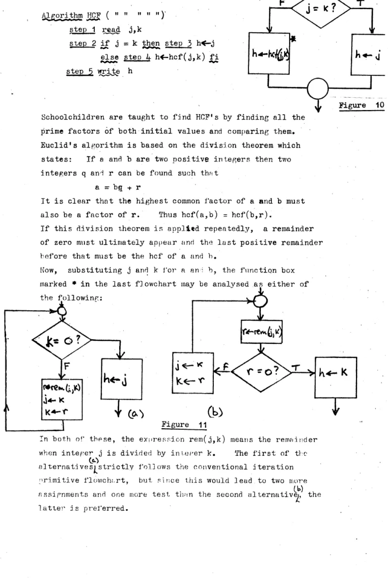
Algorithm HCF ( 11 " " " 11) step 1 read j,k
step 2 if j = k then step 3 h<-*j else steo 4 h*-hcf(j,k) fi step 5 write h
prime factors of both initial values and comparing them. Euclid's algorithm is based on the division theorem which states: If a and b are two positive integers then two integers q and r can be found such that
a - bg + r
It is clear that the highest common factor of a and b must also be a factor of r. Thus hcf(a,b) = hcf(b,r).
If this division theorem is applied repeatedly, a remainder of zero must ultimately appear and the last positive remainder before that must be the hcf of a and b.
Now, substituting j and k for a and b, the function box
k * - J
Figure 10 finding all the
marked * in the last flowchart may be analysed as either of
the following: v. r \
Figure 11
k « - K
In both of these, the expression rem(j,k) means the remainder when integer j is divided by integer k. The first of the
to
alternateves^strictly follows the conventional iteration primitive flowchart, but since this would lead to two more
Alternative (a) would be expressed as:
while k / 0 do step 5 od
step 5 do r*-rem(j,k); j«-k; k«-r od step 6 h*— j
Whereas alternative (b) would be expressed as:
step 1+ r*-rem(j,k)
step 5 if r / 0 do step 6 od fi1 * •'N— ' , ,
---step b do k; k<r-r; goto step od step 7 h*—k
The solution of rera(j,k) may be left to the final programming stage in the knowledge that in many Fortran function libraries there is a function MOD(«J,K) which is assigned the value of the remainder when J is divided by K. Y/ithout this function the expression K-(K/j)*J may be used to give the remainder since the first part of the expression to be evaluated (K/j) returns only the partial or integer quotient*
There is one further small refinement to be made to the
algorithm. If at some stage the remainder is one, there is ciearly no need to repeat the procedure and determine that the remainder at the next stage is zero. We can conclude instead that j and k are mutually prime, that is hcf(j,k) =1. With
a* A sk(7i r* ►vwiA.btred-j
X*
C_1.
Figure 12
write h read j,k
Algoritlm (Highest Common Factor) Given two positive integers j and k, find their highest common factor which is the largest positive integer, h, which divides both j and
Step 1 read j, k
Step 2 if j s k then step 3 h^— j
else do step 4: step 5 od fi Step 4 r<— rem(j, k)
Step 5 if r as 1 then step 6 h«— 1 else do step 7 od fi Step 7 if r = 0 then step 8 h*— k
else step 9 do j <- k; k<— r; goto step 4 od fi
The next stage, writing the program, will be illustrated here although it will normally be left out of the main text and put in an appendix. Coding in Algol after the final algorithmic
statement is straightforward. However, since Fortran was not designed with structured programming in view, some departures from the algorithm may be indicated* One useful device in Fortran is the three-way conditional statement IF(X)a,b,c
where a, b, and c are three branch labels according to whether X is negative, zero, or positive. This is used in the following
FUNCTION IHCF(JJ,KK) if(Jj.eq.kk) go to 5 J=JJ
IG=KK
1 L=K-(K/J)*J
IF(L-1)3,4,2 2 K=J
J=L GO TO t 3 IHCF=J RETURN 4 IHCF=1
RETURN 3 IHCF=JJ
RETURN, END
There are a few minor points to note in this function routine.
This routine will execute Euclid's algorithm for all integers.
The division theorem ensures that even for pairs of very large integers the algorithm will yield the hcf after relatively few iterations* In the application to be developed in chapter 6, however, it will rarely be used with integers greater than, say, 20. This suggests that if a difference is used instead of a remainder, the algorithm will work even more quickly.
The computation of a remainder calls for a division and a multiplication which are both computationally slow compared with a subtraction. Thus, reverting to figure 12 and substituting . r4— j - k in place of i*-rem(j,k), and then observing that this calls for j to be greater than k, the flowchart and algorithm may be revised as:
Figure 13 *
k
*-<
aK
A1 gorithm Jg£F (Highest Common Factor) Given two positive integers j and k, find their highest common factor which is the largest positive integer, h, which divides both j and k.
step 1 read j, k
step 2
J>k
$
21
2
& £ £ & £i
S te p 5 jf j = k goto step .8
else step 4 d*r»k; k>*<—j; j*-<d od fi step 5 d^—j - k
step 6 if d = 0 ggto step 8
else step 7 j*-k; k<~d; goto, step 2 gd £i step 8 h*-k
step 9 write h
Noting that the predicates in steps 2 and 3 may be implemented in Fortran by a three-branch conditional statement, this algorithm may be coded as:
FUNCTION IHCF(JJ,KK) .T=JJ
K=KK
t IF(J-K)2,4,3 2 D=K
K=J J=D 3 D=J-K
IF(D.EQ.0)G0T0 4 J=K
K=D GO TO 1 4 IHGF=K RETURN
END
The Automatic Design of Experiments
i.
Some Practical Algorithms
CHAPTER TWO
The objectives of an experiment can usually be stated in terms of a mathematical model whose parameters are .to be estimated* The best experimental design is
that set of combinations of values of the control or independent variables which will permit the estimation of those parameters with greatest precision, with
least bias, and within allowable cost limitations. A ; further criterion is expressed in terms of the use to which the fitted model will be put: the design should lead to the estimation of parameters such that the model may be used to predict values of the dependent variables with the greatest possible precision and the least bias, in a pre-specified region of the independent variables.
in a proliferation of alternative methot s of analysis, hedged about with restrictions and qualifications, to the confusion of the practical worker.
In 'Statistical Methods for Research Workers' Fisher actually encouraged the statistician to look around for the test giving the highest significance! It is not surprising that physical scientists some limes remark that they see little of relevance to their research in standard texts on experimental design and analysis (such as Fisher (1933)> Cochran and Cox (195C), and Kempthorne
(1952)).
The developing complexity of physical research has called for a different approach to experimental design based upon the estimation of effects rather than upon tests of the significance of their comparisons. Indeed, effects of treatments can no longer be estimated simply, because we are now faced with multi-parameter mathematical models which call for a more subtle approach: usually least
squares regression analysis and sometimes with ingenious coding of the variables. Furthermore, the research worker usually knows that these effects, as expressed by parameters or coefficients of the model, exist and what he needs is an efficient estimate of the parameters and reasonably accurate estimates of their errors.
Two types of variable can enter a model: qualitative and quantitative. It may be argued that quantitative
variables should be further sub-divided into continuous quantitative and discrete quantitative. For example, in making a cake one might have any continuous measure of
2.3
usually measurer] and non trolled in discrete steps. Cooks would not specify sugar more precisely than to the nearest- half ounce; steelmakers would not specify carbon content more nrecisely than the nearest 0.01 per cent.
In industrial research, where the major objective is usually the optimisation of a physical property or the cost or yield of a process, this dependent variable may he reoresenied as the response surface in the space of the independent or control variables. In many cases, the experimenter has sufficient knowledge of his process to know, not only that effects exist, but that he is close enough to the optimum he seeks to be able to assume a response surface that is quadratic in the independent variables.
'Phis situation is so common that it v/as decided for the nresent to limit the development of algorithms for the
design of continuous variable experiments to those situations which could be represented by quadratic models.
Industrial laboratories frequently arrange experiments based entirely on qualit ative variables for which there is no orior justification for ordering. None of the variables can therefore be coded so as to be analogous to discrete
quantitative variables. Such an experiment may be to assess the effects on a chemical estimation of: different laboratories; different apparatuses; different operators; different
2.4
be made is more than is practically oossible, limited nerhans by cost, time, and available materials- This problem has rherefore beer studied and algorithms have
been developed to prodnce fractions of multi-level factorial experiments.
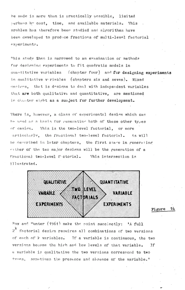
r|'hi s study then is narrowed to an examination of methods for designing experiments to fit quadratic models in
Quantitative variables (chapter four) and for designing experiments in qualitative variables (chapters six and seven). Mixed
nesi pns, that is designs to deal with independent variables that are both qualitative and quantitative, are mentioned in chanter eight as a suoject for further development.
There is, however-, a class of experimental desirn which can bn used as a Via sis for genera tin *T both of these other types of desirn. This is the two-level factorial, or more
ar-fi oii I arl v, the fractional two-level factorial. A.s will be described in later chapters, the first st.a(re in genera ling
i ther of the two matior designs will be the. generation of a fractional two-level f-ctorial. This intersection is illustrated.
Figure 14
box and TJunter (1960 make the point succinctly: ’A full k
There is a further advantage in including the fractional two-level factorial in this study: it is sufficiently simple in concept to have acquired an almost universal adoption among physical, chemical, and metallurgical research workers. They have been familiar with it
for some years, due largely to writers like Davies (1954), Duckworth (1968), and Mendenhall (1969). Yet these research workers still have problems and the most frequent is that of 1 generating the best fraction of a factorial to suit the
circumstances.
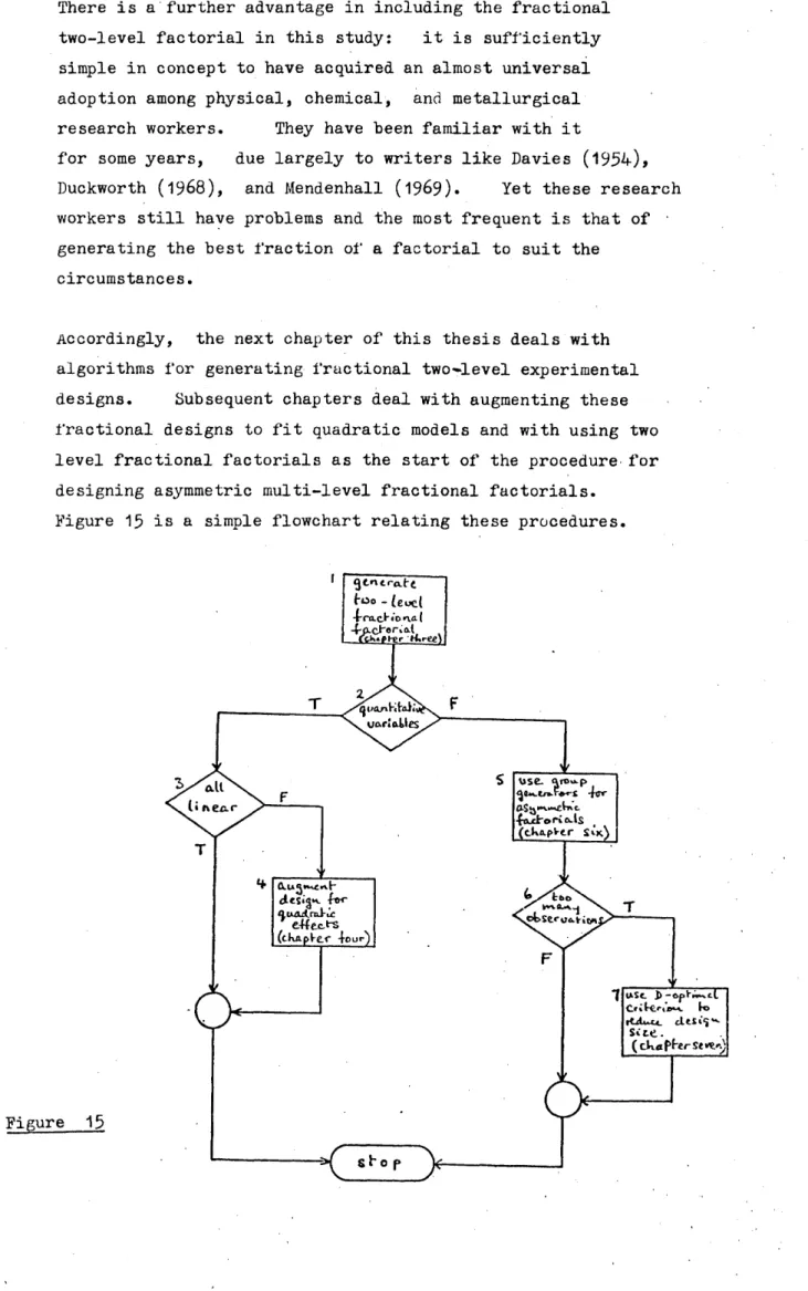
Accordingly, the next chapter of this thesis deals with algorithms for generating fractional two«»level experimental designs. Subsequent chapters deal with augmenting these fractional designs to fit quadratic models and with using two level fractional factorials as the start of the procedure for designing asymmetric multi-level fractional factorials.
The first function (box 1) in the flowchart of figure 15 is the generation of a two-level fractional factorial design using the procedure to be developed in chapter three. This follows from the argument that whether the independent variables are qualitative or quantitative, the fractional two-level design will form a base on which the more complex designs will be built.
If the variables are quantitative (box 2) and if only linear main effects and interactions are expected (box 3) then the two-level fractional factorial design satisfies the requirements.
However, if quadratic effects are expected for any of the variables, then the design must be augmented with extra observation points to allow the estimation of those quadratic terms (box 4)« The algorithms for augmentation are developed in chapter four.
If the variables are all qualitative but any of them has more than two levels, then the design is classed as an asymmetric factorial (box 5). A procedure for generating balanced fractional asymmetric factorial designs is developed in chapter six.
Sometimes a balanced fractional asymmetric design has more observations than is economically acceptable by the experimenters and is also
grossly over-determined (box 6). If this is so, then the criterion of balance is abandoned and a subset of the observations in the
balanced fraction is selected using the criterion of D-optimality (box 7). The algorithms for this are developed in chapter seven.
A natural extension of this work would be the development of algorithms for designing mixed experiments: those with both qualitative and
The Automatic Design of Experiments
Some Practical Algorithms
CHAPTER THREE
TWO-LEVEL
1
2
3
FACTORIALS
Background
Algorithms
1 Background
The early papers by Fisher (1926 et seq) and Yates (1933 et seq) stimulated a steady flow of papers on both the design and analysis of factorial experiments. Their ability to be divided into blocks by confounding high order interactions with block effects appealed particularly to the agricultural statisticians and they were helped by Barnard (1936) who enumerated a selection of confounded arrangements.
These enabled the research.worker to choose a design by inspection but they did not give him a uniform procedure for ensuring that his choice would provide the conditions for estimating all the required coefficients of the model to be fitted. Indeed there seems to be little in the literature before the 1950's which discussed explicit mathematical models when considering experimental design.
Finney (1948) drew attention to this in a paper which described the estimation and interpretation of main effects and interactions. He commented: "few things betray the inexperienced statistician more readily than a triumphant presentation of an elaborate analysis of variance table coupled with an almost complete neglect of treatment means."
One of Finney's major contributions was his clear exposition (1945 and 1946) of the relationship between block confounding and fractions of two level factorials. In these papers he explains the notation introduced by Fisher and Yates and which, through common use, has been accepted generally as standard.
two levels, the factors would be named A, B, and C. The effects of these factors would also be labelled A, B, and C: the first order interaction effects would be labelled AB, AC, and RC; and the second order interaction effect would be labelled ARC. An objective of the experiment would be to estimate these effects together with the mean effect which is denoted by I. Combinations of lower case letters denote firstly experimental desirn points. For example: ac represents the observation point at which factors A and C are both at their high levels and factor B is at its low level. The case where all f; ctors are at their low l.vels is denoted by (l). This lower case notation is also used, without confusion, to represent the observed
values of the dependent variable at the corresponding observation points.
As well asra standard notation, there is a standard crder for lisfinr observation points and factorial effects. The standard order is clear from the following example, with three factors:
This standard not.ationai order will be shown to have value in the next section when the design algorithms are developed.
Observation points Factorial effects
I
a A
b B
ab AB
c C
ac AC
be BC
ABC
In the same paper, Finney stated: "In planning a 2n experiment, using only 2? treatment combinations in a l/^n-p replicate, the first step is t. select a suitable alias subgroup of
n-p
3.3
sub-group of this as the set of treatment combinations."
The "alias sub-group" to which he refers is also known as the "set of defining contrasts''^ which will be described later^ and their selection constitutes the outstanding problem in designing fractional two-level factorial experiments. Finney gave no formal procedure for choosing the defining contrasts. In his
example he arbitrarily chose some with high resolution (interactions
b e t w e e n more than three factors) and then tested, that they would
not. lead to aliasing between main effects and low order interaction effects.
He did, however, describe a formal procedure for developing a fractional design once a suitable set of defining contrasts had been chosen. This procedure followed the demonstration by
Hi: her (194-i) of the connection between confounding and the theory of Abelian groups. This connection is shown to be of value in the next section of this chapter when the implementation of the design algorithms as computer programs is described. It is shown to have further value in the algorithms for designing fractional mixed multi-level factorials which are described in char'ter seven.
Kempthorne (1947) offered an alternative notation for the design points, using ones and zeros. He also described factors by lov/er case sub-indexed x's: "If the factors are x^, x^, . •
J.4
kempthorne also illustrated the procedure for designing fractions once a suitable alias sub-group or set of defining contrasts had been chosen; but, he admitted, "no simple method has been found of enumerating such groups."
Box and Hunter (1961) gave a thorough treatment of the notations, design, and analysis of fractional factorial experiments and
they suggested a procedure for choosing a set of defining contrasts in a less than wholly arbitrary way. They defined the resolution of a design as the smallest number of factors represented in the design's set of defining contrasts. The resolution of a design would influence the degree of confounding of effects, when they came to be estimated from the observations, as follows:
In designs of resolution 3, no main effect would be confounded wii.h any other main effect, but main effects would be confounded with two-factor interactions.
In designs of resolution 4, no main effect would be confounded with any other main effect or any two-factor interaction, but two-factor interactions would be confounded with each other.
Tn designs of resolution 5, no main effect or two-factor interaction would be confounded with any other main effect or two-factor
interaction, but two-factor interactions would be confounded with three-factor* interactions..
V/ it1, these re sol ulm '%ns in mind they suggested the foil owing procedure for choosinr a suitable set of defining contrasts: alias the main effects and required interactions with other
The procedure of Box and Hunter was hot, however, a direct path from an explicit statement of the model to be estimated to the choic of a suitable set of defining contrasts* Nor was the similar procedure of Whitwell and Morbey (1961) who dealt specifically with designs of resolution five since these would certainly lead to the estimation of all first order interactions as well as main effects. Their argument rested on the assumption that all first order interactions were needed. They did not
consider questioning the experimenter's model to discover if
there could be any a priori discarding of first order interactions.
Addelman (19&3) reviewed known techniques for constructing fractional designs. He commented: "The crucial part of the specification of a fractional replicate plan is the choice of the defining or identity relationship. One should always attempt to choose interactions for the identity relationship in such a way that those interactions that are completely confounded with the effects or interactions that one wishes to estimate are negligible"
The advocacy of authors such as Cochran aiid Cox (1950), Kempthorne (1952), Brownlee (1953), Davies (1954),
Duckworth (1968), and Mendenhall (I9t>9), led to the two-level factorial becoming the most commonly used type of experimental design in industrial laboratories. Research workers generally and easily appreciated that fractions of these designs would achieve economies in both money and time spent on investigations. The advocates warned, however, that care must be exercised in the choice of these designs so as to avoid the aliasing of main effects and important interactions.
The usual procedure is to refer to a standard textbook and try to pick a published design to meet the experimental needs. If a
suitable design is not found, a research worker with some understanding of the subject will try a few arbitrary sets of defining contrasts, generating aliasing matrices until a suitable design is found. This introduces an undesirable element of
arbitrariness. A paraphrase of the procedure recommended in man^texts is:
"First choose a suitable set of defining contrasts. Secondly use these defining contrasts to generate an aliasing matrix and check if all the main effects and interactions that need to be estimated can be estimated without being aliased with any others. If this check fails, start again. If it passes: thirdly use the defining contrasts to generate the fractional design."
The procedure given for the final stage is satisfactory, but that for the first is no more than guesswork. The outstanding problem, that has not previously been solved, is to establish a logical and easy procedure to select a set of defining contrasts: that define an aliasing matrix in which the experimental requirements are not aliased.
This is not a trivial problem . It is not uncommon for a research worker to spend several days searching for a suitable set of defining contrasts by trial and error. In view of this, and in view of the historical awareness of the importance of the problem, the simplicity of the solution comes as a surprise. The purpose of this chapter is to explain the solution which has been published in a brief form, Greenfield (1976). After publication, Franklin (1977) identified a case where my algorithm gave an incorrect answer and I immediately submitted a modification for publication (1978). Meanwhile, Franklin and Bailey (1977) developed and published an alternative algorithm, which has the added advantage, for agricultural work in which their main interest lies, that it can lead to division of a fractional
2 Algorithms
The object of the algorithms to be developed in this section is to design a fractional two-level factorial experiment that will admit the estimation ofthe coefficients of a prior stated linear relationship between a dependent variable and a set of independent variables. The latter may be.described as the a
main effects and some of the interactions of a set of factors. In the.earliest version of these algorithms interactions were restricted to first order: those between two factors. This was supported by Box and Hunter (1961) who wrote: "With continuous variables it is reasonable to expect the response to vary smoothly. With qualitative variables certain aspects of similarity may be expected in the responses at the.different versions. . . . In the conditions of smoothness and
similarity commonly encountered, three, factor and multi-factor interaction effects are often negligible." However, in subsequent applications there have been several cases where second order interactions, those between three factor*, have anticipated for physical reasons. Thus'the al gorithms must allow the inclusion of interactions of any order. This is a marked departure from the procedures for producing designs of resolution 3, 4 or 5*
The full algorithm may be divided into.three main steps: 1. Enter the requirements set: those main effects and
interactions which are required to be estimated;
2. Determine the fraction, size and find the defining contrasts 3. Generate and print the design.
Since the second step of the full algorithm has historically been the most taxing, the algorithmic solution will be
The problem is to find a set of defining contrasts which will define a fractional design that will allow the unaliased estimation of all the elements of the requirements set. The solution to the problem is to generate the defining contrasts and the aliasing matrix together, instead of first one and then the other. Effectively this is done by a tree search which is most easily described in terms of an example. The algorithm will first, be- expressed in strai ghtforward English interspersed with the steps applied to an'example. It will then be developed more formally.
5
Consider a 2 experiment in'which the variables are labell ed -',B,C,D,E. What is required is the small estpossible balanced fractional design that can be used to estimate each of the main effects an' also the effects of the first-order interactions AB and AE, assuming that the effects of all other interactions on the dependent variable are known in advance to be negligible. The requirements set is: A,B,AB,C,D,E,AE . The design must
also estimate the mean, so in this case there must be a minimum of eight observations.
Algorithm tyjpfpj\[ fuEFining CONtrasts) Sten 1. Find m such that 2n m ^ 1 + n - i p
where n is the number of factors, p is the number of in the requirements set.
interactions / if the procedure shows that there is no unaliased design of the size determined by the above expression, it continues to a fraction of double the size. That is m is decreased by one. In the example, the first value of m is 2, so the smallest fraction likely to provide a suitable design is a quarter.
Step 2. Find the (n-m) majority factors in the requirements set.
These are the factors that occur most frequently in the
Step 3» Write the first column of the aliasing matrix in terms of the (n-m) majority factors. This has 2n m element (eight in the example). Mark with an asterisk those elements common to this column and to the requirements set.
Example:
First column of the aliasing matrix:
I A* B* AB* E* AE* BE ABE
The requirements set: (A*,B*,AB*,C,D,E*,AE*)
Step 4. Generate the first defining contrast by taking the product (modulo 2) of the last available element in the first column and the last available element in the requirements set.
Example: ABE x D = ABDE
Step 5. Use this defining contrast to generate the next column of the aliasing matrix. Check at the same time if any of the required effects have become aliased with those already marked in the first column. If not, mark those that have been introduced.
Example:
The requirements set is:
(a*.b*;a b*,e*,a e*,c, d*)
First. Second column column
I ABDE
A* BDE
B* ADE
AB* DE
E* ABD
AE* BD .
BE AD
between required effects
Step 6. If any aliasingoccurred in step return to step 4. generating a new first defining contrast by taking the product (modulo 2) of the next from last available element in the first column and the last available element in the requirements set. In the present example this does not occur.
Step 7..When the* are no more available elements in the first column, and if the requirements have not all been met, decrease m by one and return to step 5.
Step 8. Generate the next defining contrast as in step 4. Example: BE x C = BCE
As will be explained later, this leads automatically to the third defining contrast as the product of the first and the second.
Example: ABDE x BCE = ACD
Step 9« Generate the full aliasing matrix, mark with asterisks and check for aliasing as in step 5.
Example:
Column 1, Column 2 Column 3 Column
I ABDE BCE ACD
A* BDE ;ABCE ‘ CD
B* ADE CE ABCD
AB* DE ACE BCD
E* ' ABD BC ACDE
AE* BD ABC CDE
BE AD C* ABODE
ABE D* AC BCDE
The requirements set is (A*,B*,AB*,K*,AE*,C*,D*)
The algorithm described above is sufficient to be followed
The connection between confounding and Abelian groups was ^described by Fisher (1943)* This connection becomes more
notable when a binary digit coding is adopted for both the treatment combinations (design points) and main effects and interactions,. especially since digital computers use binary integers. In the code adopted here, the binary digits, or bits, are read ard counted from right to left. Thus:
00000010 b B or b (bit 2 is described as 'up','set'
or 'one1)
00000101 = AC or ac (bits 1 and 3 are set)
Since this coding will be used in the programs but alphabetic coding is preferred for human reading, an algorithm will be needed to convert from binary code to aphabetic code. This will be described later as part of algorithm ALMAT (print- ALiasing MATrix).
The binary code permits the direct generation of two-level factorials by counting upwards from zero as follows:
Denary count Binary oode Treatment combinations 0 1 2 3 4 3 6 7 8 9 10 11 12 • etcetera
The table stops at the denary count of 2n - 1, where n is the number of factors.
00000 (1,)
00001 a
00010 b
00011 ab
00100 c
00101 ac
00110 be
00111 abc
01000 d
01001 ad
01010 bd
01011 abd
The product of any two elements (modulo 2) when using the binary code is seen by an example:
ABDE x BCE = ACD is equivalent to 11011 x 101,10 = 01101 It is convenient that this can be achieved by the use of the exclusive-OR operator (referred to in future simply as eor) which is defined by the following truth table:
A B eor (A,B)
0 0 0
1 0 1
0 1 1
1 1 0
As Fisher noted, the full factorial design and, the full aliasing matrix (see example after step 9 above) are both groups of order 2n under the product (modulo 2) operator. Similarly if a full design on n factors is expressed as the set of integers from
0 to 2n - 1 in binary code, then the set becomes a group under the exclusive-OR operator.
If D = the set (0,1, . . . , 2n-l), then for all x C D and for all yC D there is a z£D such that eor(x,y) = z.
The group's identity element is 0, since for all x£ D eor(0,x) = eor(x,0) = x
Also every element x has an inverse which is itself: eor(x,x) = 0 (the identity)
As an example let n = 2,
then D = ((l),a,b,ab) in alphabetic code or D = (0,1,2,3) in denary code
or D = (00,01,10,11) in binary code
Application of the operator to all ten pairs is seen to always yield members of D:
eor(00,00) = 00 eor(00,01) = 01 eor(01,10) = 11
3.13
It is also useful to note that as well as the full aliasing matrix being a group, using the binary notation and the exclusive-OR operator:
* the first column of the aliasing matrix is a sub-group * the first row of the aliasing matrix (which is the full
set of defining contrasts including the identity) is a sub-group
* the fractional design that will be derived using the defining contrasts is a sub-group of the full design group.
One difficulty that has been met in implementing these algorithms on various computers is that in standard Fortran the exclusive-OR
(and other logical., operators). n TT
operator/can T5e used onlyrwith logical operands. However, on some scientific computers, such as the IBM 1130 and 1800 and the OA SPCl6r logical operators can also be used with integer operands to give an integer result. The integer operands arq considered
to be in their binary representation as described here. The result reflects whether corresponding bits in the two operands are set or not.
The related types of operator will be distinguished here by different notations, acting on logical operands P and Q and on integer operands I and J:
Logical operators: P.xor.Q P.or.Q P.and.Q
Binary integer operators: eor(l,j) or(l,$) and(l,J)
There should be no objection to using these binary integer operators. hven if they are not provided with the high level language function library, any competent programmer should be able to write them using a machine code or assembler language, and add them to the function library.
a further useful feature of the group property described is that
3.14
are expressed in standard order (counting from 0 to 2n-1 in the case of the full design or its equivalent order for a sub-group as illustrated by the first column of the aliasing matrix in the earlier example) or in the order in which they are created (as in the first row of the aliasing matrix: the defining contrasts), , then:
the generators are those elements in the positions with order numbers 2+1, where r is any integer 0, 1, 2, . .
As an example, consider the full factorial with n = 3* The elements of the factorial will be expressed alphabetically for reading clarity. The order numbers are, set below. The genenator are marked with asterisks.
(1) a b ab c ac be abc
1 2 3 4 5 6 7 8
* * *
In this case the answer is obvious because the generators are those elements with single letters. However the rule may not seem so obvious when generating the set of defining contrasts and in the algorithm for doing this the rule is of particular value.
Tt is used as follows: when the elements of a group or sub-group are developed from left to right (in the above example), every time a generator is created the remaining elements of the group un to, but not including, the next generator can be created by taking the product of the new generator with each of its preceding elements in turn.
In the example above, the first element to be written is (l).
The first generator to occur is a. Aoplication of the prodedure described creates the single element a.
The second generator to occur is b. Application of the procedure creates the elements b and ab.
Returning now to the earlier example: consider the first row of the aliasing matrix as a sub-group.
The first element to be written was the identity I.
The first defining contrast to be created (by taking the product ABE x D) was ABDE. This is the first generator and it creates the element of the sub-group ABDE.
The second defining contrast to be created (by taking the product BE x C) was BCE. Application of the procedure described creates two new elements of the sub-group:
BCE (which is BCE x i) and ACD (which is BCE x ABDE).
The rule for identifying a new generator is useful in the main algorithm in three ways; First, after the majority factors have been identified, it leads to the use of the above generating procedure for generating the first column of the aliasing matrix.
Second, when a new defining contrast is created it leads to the use of the above procedure for generating consequent defining contrasts.
Third, it helps in designing a marking, or flagging, system so that if aliasing is discovered after a defining contrast has been created the algorithm can backtrack to the previous generator defining contrast. The method and value of this use will become clearer as 1he algorithm unfolds. It may be, noted here that a simple aid in back tracking is:
if Y is the order number of the current generator (for example, if r = 5 then Y = 2r+1 =■ 33)
and if X is the order number of the previous generator, then to determine X it is simpler to write X<-(Y-l)/2 than to compute r from Y and then, by decrementing r,
r to compute X from 2 +1.
In the earlier description of the general algorithm DEFCON,
than through the use of simple marks like asterisks has to be developed for a programmable algorithm. Discussion of the procedure and the development of the algorithm will be helped by now defining some of the variables to be used; Practical dimensions of arrays are denoted by (*n).
MV(l) = the Ith element of the requirements set (*32) NV = the number of elements in MV
N the number of two-level factors
M = the fraction index (the design would be a 1/2^ factorial) K(l,J)s= the I, Jth element of the aliasing matrix (*128 x 32)
number of rows in the aliasing matrix number of columns in the aliasing matrix defining contrast being tested for acceptance
column number of the defining contrast being tested column number of the current generator defining contrast a marker for the Jth element of the requirements set (*32) 0 if accepted
100 if currently not being considered
the value that LNEW had when the Jth element of the requirements set was tentatively accepted
a marker for the Ith row of the aliasing matrix (*128) 1 if the row has definitely been assigned
0 if the row has been tentatively assigned -1 if the row is still available
another marker for the Ith row of the aliasing matrix (*128) 0 if the row has definitely been assigned
100 if the row is still available
the value that LNEW had when the Ith row of the aliasing matrix was tentatively assigned
a copy of the Jth element of the first row of the
aliasing matrix: to save reference time when computing (*32) the n factors expressed in majority order (*16)
a temporary array used in producing MAJ(l) (*16)
A function subprogram NEW(l) will be called to test if I has a I*
value of 2 +1, where r is any integer. NF
NI KEST = JAK = LNEW = IN(J) =
IV(I) =
KR(I) =
KK(J) =