Generalized Exponentiated Moment Exponential Distribution

e-Publications@Marquette

Mathematics, Statistics and Computer Science

Faculty Research and Publications

Mathematics, Statistics and Computer Science,

Department of

10-1-2014

Generalized Exponentiated Moment Exponential

Distribution

Zafar Iqbal

National College of Business Administration and Economics, Lahore

Syed Anwer Hasnain

National College of Business Administration and Economics, Lahore

Muhammad Salman

National College of Business Administration and Economics, Lahore

Munir Ahmad

National College of Business Administration and Economics, Lahore

Gholamhossein Hamedani

Marquette University, [email protected]

Published version.

Pakistan Journal of Statistics,

Vol. 30, No. 4 (October 2014): 537-554.

Publisher

link

. © 2014 Pakistan Journal of Statistics. Used with permission.

© 2014 Pakistan Journal of Statistics 537

2014 Vol. 30(4), 537-554

GENERALIZED EXPONENTIATED MOMENT EXPONENTIAL DISTRIBUTION

Zafar Iqbal1, Syed Anwer Hasnain1, Muhammad Salman1 Munir Ahmad1and G.G. Hamedani2

1 _{National College of Business Administration & Economics} Lahore, Pakistan.

Email: [email protected]; [email protected] [email protected]; [email protected] 2 _{Department of Mathematics, Statistics & Computer Science}

Marquette University, Milwaukee, WI 53201-1881, USA Email: [email protected]

ABSTRACT

Moment distributions have a vital role in mathematics and statistics, in particular in probability theory, in the perspective research related to ecology, reliability, biomedical field, econometrics, survey sampling and in life-testing. Hasnain (2013) developed an exponentiated moment exponential (EME) distribution and discussed some of its important properties. In the present work, we propose a generalization of EME distribution which we call it generalized EME (GEME) distribution and develop various properties of the distribution. We also present characterizations of the distribution in terms of conditional expectation as well as based on hazard function of the GEME random variable.

KEYWORDS

Survival function; hazard rate function; information generating function; characterizations.

1. INTRODUCTION

If F x

 

is a cdf (cumulative distribution function), then [ ( )]F x  is a cumulative

exponentiated distribution (ED) function, where  0 is the exponentiated parameter. Rao (1965) extended the basic idea of Fisher (1934) and introduced moment or weighted distributions. The moment distribution deals in the perspective of unequal probability sampling. Gompertz (1825) used the cdf to compare the known human mortality tables and represented population growth, i.e., (1 _e x ) _{Later on, Gupta et al. (1998)}

introduced a distribution by setting  1. To study the theoretical properties of Gompertz (1825) family, three parameters of location, scale and shape were introduced to generalize exponential distribution in comparison with gamma and Weibull distributions, (see also Gupta and Kundu, 1999, 2000, 2001, 2004 and 2005 where they discussed various properties of [ ( )]F x ). Gupta and Kundu (2005) estimated P X



Y



, where X

Employing exponentiated gamma distribution, Shawky and Bakoban (2008) studied the lower record values and derived explicit expressions for the single, product, triple and quadruple moments. Raja and Mir (2011) conducted a numerical study by taking the eight distributions namely gamma, Weibull, lognormal, Gumble, exponentiated Weibull, exponentiated exponential, exponentiated lognormal and exponentiated Gumble and have fitted the distributions to two real life data sets.

Dara (2012) proposed cdf of moment exponential distribution and developed some basic properties such as moments, skewness, kurtosis, moment generating function and hazard function. Hasnain (2013) proposed exponentiated moment exponential (EME) distribution with cdf given by

 

1 1 e 0 x x F x x     _{ }      _{ }   _ _    (1.1)

where  and  are positive real parameters, and established certain properties of EME distribution.

The presentation of the content of this work is as follows: Section 2 deals with cdf and

pdf (probability density function), survival function, hazard rate function and graphs for GEME distribution. Moments, mode, median, information generating function of GEME distribution are discussed in Section 3. In Section 4 certain characterizations of GEME distribution are presented in terms of conditional expectation and hazard function. Some remarks are presented in Section 5. An empirical study has been conducted and discussed in Section 6 and tables of percentile for selected values are given in Section 8. Finally concluding remarks are provided in Section 8.

2. PROPERTIES OF GENERALIZED EXPONENTIATED MOMENT EXPONENTIAL DISTRIBUTION

We introduce the GEME distribution with cdf given by

 

1 1 e 0 x x G x x       _{ }      _ _ _{ }    _{ }    (2.1)

where  , and  are positive real parameters.

The three-parameter GEME distribution will be quite effectively used in analyzing several lifetime data, particularly in place of parameter gamma distribution, three-parameter Weibull distribution or three-three-parameter exponentiated exponential distribution. The GEME distribution produces many distributions via special transformations.

The pdf of GEME distribution is

 

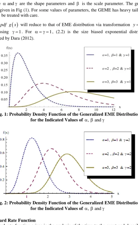
1 2 1 2 1 1 e e 0, , , >0 x x x g x x x           _{ }       _  _ _{ }       _{   }   (2.2)

Here  and  are the shape parameters and  is the scale parameter. The graph of (2.2) is given in Fig (1). For some values of parameters, the GEME has heavy tail which needs to be treated with care.

The pdf g x

 

will reduce to that of EME distribution via transformation yx or by choosing  1. For    1, (2.2) is the size biased exponential distribution developed by Dara (2012).

Fig. 1: Probability Density Function of the Generalized EME Distribution for the Indicated Values of  , and 

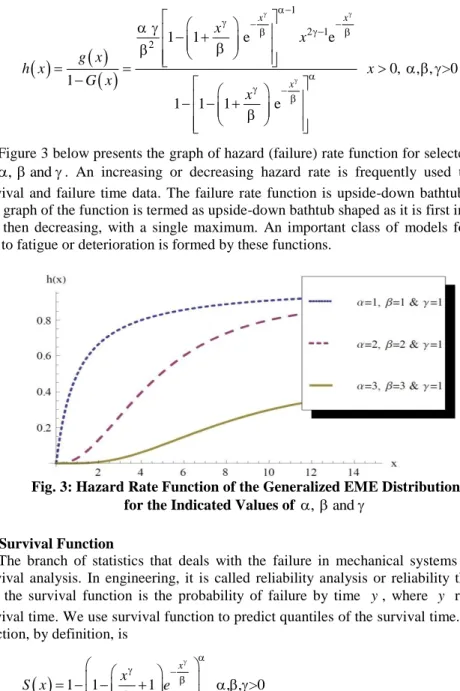
Fig. 2: Probability Density Function of the Generalized EME Distribution for the Indicated Values of  , and 

2.1 Hazard Rate Function

Hazard rate function arises in the analysis of the time to the event and describes the current chance of failure for the population that has not yet failed. This function plays a pivotal role in reliability analysis, survival analysis, actuarial sciences, demography, extreme value theory and duration analysis in economics and sociology. It is very

important for researchers and practitioners working in the areas like engineering statistics and biomedical sciences. Hazard rate function is very useful in defining and formulates a model when dealing with lifetime data.

For the GEME distribution, hazard rate function takes the form

 

 

_{ }

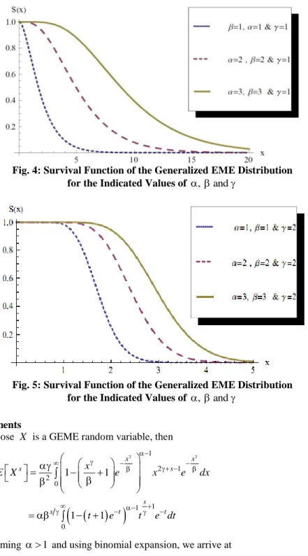
1 2 1 2 1 1 e e 0, , , >0 1 1 1 1 e x x x x x g x h x x G x x                _{ }     _{  }        _{   }          _{ }       _ _{ } _{ }       (2.3)

Figure 3 below presents the graph of hazard (failure) rate function for selected values of  , and . An increasing or decreasing hazard rate is frequently used to model survival and failure time data. The failure rate function is upside-down bathtub shaped. The graph of the function is termed as upside-down bathtub shaped as it is first increasing and then decreasing, with a single maximum. An important class of models for failure due to fatigue or deterioration is formed by these functions.

Fig. 3: Hazard Rate Function of the Generalized EME Distribution for the Indicated Values of  , and 

2.2 Survival Function

The branch of statistics that deals with the failure in mechanical systems is called survival analysis. In engineering, it is called reliability analysis or reliability theory. In fact the survival function is the probability of failure by time y, where y represents survival time. We use survival function to predict quantiles of the survival time. Survival function, by definition, is

 

1 1 1 , , >0 x x S x e       _{ }      _ _  _{ }      _{ }   

Fig. 4: Survival Function of the Generalized EME Distribution for the Indicated Values of  , and 

Fig. 5: Survival Function of the Generalized EME Distribution for the Indicated Values of  , and 

2.3 Moments

Suppose X is a GEME random variable, then

1 2 1 2 0 1 1 x x s x s E X e x e dx             _{ }      _{    }   _ _ _{ } _ _  











1 1 0 1 1 s s _{t e}t _t_{e dt}t  

_

 

 





 

/ / 2 1 1 / 2 1 1 , , 0 1 i _i s s j s i j j s i E X i j _i                 _{  }  _{  }      

 

_{   } (2.4)

Since (2.4) is a convergent series for s0, all the moments exist for integer values of

. The equation (2.4) can be represented as a finite series representation. Therefore, by setting different values of s1, 2,3 and 4, we obtain the first, second, third and fourth moment about zero.

2.4 Information Generating Function

The information generating function for GEME distribution is

 



 



1



 



0 s s H f E f X f x dx      _{ }  



  









2  1 0 0 1 1 2 , 0 i _{i s j} s s i j s i s j s i j i  _{ }            _  _{ }       

 

(2.5)

The Shannon entropy can be found by

 

1

s

d H f ds  .

2.5 Factorial Moments and Mode

The factorial moments of GEME distribution random variable X are as follows





 







 

 

0 1 2 ... 1 r , k k E X X X X r S r k E X      



for rZ

where S r k

 

, is the Stirling number of first kind and E X

 

k is defined at (2.4). The mode of GEME distribution is found by solving g x

 

0 or









2 2 1 2 1 0 1 1 x x e x x x e                     _{ }  _{   }    _       (2.6)

When  1, the mode equation reduces to 2 1 0

x x x x e  e                       , which

provides mode(s). The modes are being showed graphically for different values of

, and

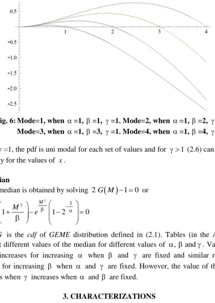
Fig. 6: Mode=1, when =1, =1, =1. Mode=2, when =1, =2, =1. Mode=3, when =1, =3, =1. Mode=4, when =1, =4, =1.

For =1, the pdf is uni modal for each set of values and for  1 (2.6) can be solved iteratively for the values of x.

2.6 Median

The median is obtained by solving 2 G M

 

 1 0 or

1 1 1 2 0 M M e   _               _  _{ }   _{ } (2.7)

where G _{is the} cdf of GEME distribution defined in (2.1). Tables (in the Appendix) represent different values of the median for different values of  , and . Value of the median increases for increasing  _when  and  are fixed and similar results are obtained for increasing  when  and  are fixed. However, the value of the median decreases when  increases when  _and  are fixed.

3. CHARACTERIZATIONS

In designing a stochastic model for a particular modeling problem, an investigator will be vitally interested to know if their model fits the requirements of a specific underlying probability distribution. To this end, the investigator will rely on the characterizations of the selected distribution. Generally speaking, the problem of characterizing a distribution is an important problem in various fields and has recently attracted the attention of many researchers. Consequently, various characterization results have been reported in the literature. These characterizations have been established in many different directions. The present work deals with the characterizations of GEME distribution based on: (i) conditional expectation of certain functions of the random variable; (ii) hazard function of the random variable.

3.1 Characterizations based on Conditional Expectation Proposition 3.1.1

Let X: 

 

a b, be a continuous random variable with cdf G and pdf g. Let

 

,

C a b

  and C1

 

a b, such that

 

   

b a u du u u       



and g a

 

0. Then

 



|



 

, t

 

, E  X X  t t  a b (3.1.1) implies

 

exp

_{   }

 

, b x t G x dt x a t t     _ _     



 (3.1.2) Proof: From (3.1.1) we have

   

   

G , for t

 

, t a u g u du t t a b    



Differentiating both sides of the above equation with respect to t and using

 

0 g a  we have

 

 

   

 

g t t G t t t       (3.1.3)

Now, integrating both sides of (3.1.3) from x x



a



to , we arrive at (3.1.2).

Remarks 3.1.2:

(a) Let X_1,nX_2,n ... X_{n n,} be n order statistics from a continuous cdf G. In view of Proposition 3.1.1 we can make the following statement in terms of certain functions of the nth order statistic. Under the conditions of Proposition 3.1.1,



n n,



| n n,

 

,

 

, E_ X X t_  t t a b Implies

 

exp

_{   }

 

, b x t G x dt x a t t     _ _     



 (b) Taking

  

a b,  0,



,

 

1 x x x e         _  _    and

 



 



1 1 1 x x       , we have from (3.1.2)

 

1 1 , 0. x x G x e x       _{ }    _ _  _        

This gives a characterization of GEME distribution in terms of the conditional expectation of a special function of the GEME distribution random variable X. (c) One can use (a) above to give a characterization of generalized EME distribution in

terms of the conditional expectation of certain function of the nth order statistic.

Proposition 3.1.3.

Let X: 

 

a b, be a continuous random variable with cdf G and pdf g. Let

 

1

,

C a b

  be a non-increasing function such that lim

 

1

xa x   and lim

 

0 xb x   then

 

| (1- ) ( ), ( , ), E_ X Xt_ c c  t t a b (3.1.4) where 0 c 1, implies

 

1

 

1 , c c G x x x a      _{ }  (3.1.5) Proof: From (3.1.4) we have t 1 ) for

aψ (u)g (u)du = (c + ( - c ψ (t))G(t) , t (a,b)



Differentiating both sides of the above equation with respect to t results in

 

 





 

  



1 1 g t c t G t c t      (3.1.6)

Now, integrating both sides of (3.1.6) from x x



a



to , we arrive at (3.1.5)

Remarks 3.1.4: (d) Taking

  

a b,  0,



,

 

1 x x x e         _  _    and 1 1 c   , we have from (3.1.5)

 

1 1 e , 0 x x G x x       _{ }      _ _ _{ }        

This also gives a characterization of GEME distribution in terms of the conditional expectation of a special function of the GEME distribution random variable X. (e) Statements similar to (b) and (c) of Remarks 3.1.2 can be given here as well.

3.2 Characterization based on hazard function

For the sake of completeness, we state the following definition.

Definition 3.2.1

Let G be an absolutely continuous distribution with the corresponding pdf g. The hazard function corresponding to G is denoted by n_G and is defined by

 

 

, 1 G g x n x SuppG G x    (3.2.1)

where Supp G is the support of G.

It is obvious that the hazard function of twice differentiable function satisfies the first order differential equation

 

 

 

 

, G G G n x n x x n x    

where 

 

x is an appropriate integrable function. Although this differential equation has an obvious form since

 

 

G

 

 

G

 

G g x n x n x g x n x     (3.2.2)

for many univariate continuous distributions (3.2.2) seems to be the only differential equation in terms of the hazard function. The goal of the characterizations based on hazard function is to establish a differential equation in terms of hazard function, which has as simple form as possible and is not of the trivial form (3.2.2). For some general families of distributions this may not be possible. Here we present a characterization of the GEME distribution based on a nontrivial differential equation in terms of the hazard function.

Proposition 3.2.1

Let X: 



0,



be a continuous random variable. The pdf of X is (2.2) if and only if the hazard function n_G

 

x of

 

1

( )

G x  F x _  0 satisfies the differential equation

 

2





2 1 2

 

2 1 , 0 G G n x  _   x   x_n x x  _  _ (3.2.3) for ,  0. Proof:

If X has pdf (2.2), then clearly (3.2.2) holds. Now, if (3.2.3) holds, then

 

 









2 2 2 2 1 1 , G G n x x x n x              

from which we have

 

2 1 2 1 1 , G x x n x       _  _  _  _ or

 

1 2 1 2 1 G x n x x        _  _   _{ } (3.2.4)

Integrating both sides of (3.2.4) from 0 to x , we arrive at

 





2 1 2 0 ln 1 1 u x u u e G x du u e                    _   



 





2 1 2 0 ln 1 1 u x u u e G x du u e                    _   



ln 1 x x e      _{ }     _ _  _       

From the last equality, we obtain

 

1 1 x x G x e         _  _   

from which, we have

 

 

1 1 e , 0 x x F x G x x      _   _ _   _{ }   _ _ _{ }    _{ }    Remark 3.2.2

Note that G x

 

is an exponentiated cdf with base cdf F x

 

and the exponent 1

.

4. MAXIMUM LIKELIHOOD ESTIMATOR OF GEME DISTRIBUTION’S PARAMETERS

In what follows, we discuss the estimation of the LL (Log Likelihood) class parameters. Let X X₁, ₂,...Xn be a random sample with observed values x x1, 2,...,xn

from GEME distribution. Let     



, ,



be the parameter vector. The LL function based on the observed random sample of size n is obtained from





1 2 1 2 1 , , , 1 1 e e , x x n n _n obs _n j x l x x            _{ }    _{ }     _  _ _{ }  



_   _ (4.1) and













ln l , , ,x_obs n ln 2 lnn nln 2 1 lnx x               







1



ln 1 1 e x x      _{ }       _  _ _{ }       



(4.2)

Taking partial derivatives with respect to  , and  respectively from

 

4.2 , we have









ln , , , ln 1 1 e x obs l x _{n x}          _   _   _  _ _{ }   _  _    



(4.3)









2 2 ln l , , ,x_{obs n}        













2 2 3 ln , , , 2 1 e 1 1 e x obs x l x _{n x x} x                         _{ }   _{  }     _  _     



_

(4.4)













2

 

2 2 ln , , , 2 ln 1 ln e 1 1 e x obs x l x n x x x x x                        _{ }   _{  }     _  _     



_









  

2



 

2 2 2 2 2 2 3 2 ln , , , 2 ln 1 ln 1 1 x obs x l x n x x x x e x e                        _{ }    _{  }     _{  }     





 





2 2 2 1 + ln x x x x x e       _{ } _   



_  _ (4.5)

From (4.3) the asymptotic variance of  when and are fixed  is

 









2 2 2 1 ˆ ln , , , obs V n l x E                 

The MLE (Maximum Likelihood Estimate) of , say ˆ , is obtained by solving the nonlinear system. The solution of this nonlinear system of equations does not have a closed form, but can be found numerically by using software such as MATHEMATICA, MAPLE and R.

For interval estimation and hypothesis tests on the model parameters, we require the 3×3 information matrix containing second partial derivatives of (4.3)–(4.5) Under the regularity conditions stated in Cox and Hinkly (1974), that are fulfilled for our model whenever the parameters are in the interior of the parameter space, we have that the asymptotic distribution of n

 

  ˆ to be a multivariate normal N₃



0,A1

 





, where

 

 

1

n

lim_n

A   _I  is the information matrix.

We conclude this section by expressing ˆ in terms of a random variable T whose distribution will be derived in the next section.

ˆ ln 1 1 x n n T x e           _{ }   _{  }     _  _     



where 1 ln 1 1 ln 1 1 x x x x T e e           _{ }   _{ }         _  _ _{ } _  _ _{ }              





5 DISTRIBUTIONS OF T_i AND T

The following remarks and a theorem illustrate the distributions of T_i and T_.

5.1 Remarks

The following conclusions can be obtained easily which we present them as remarks.

1) If X ~GEME distribution

 

 , with  known, then ln 1 1

x i x T e      _{ }      _  _ _{ }        follows Exp

 

 .

2) T~Gamma

 

,n T~GEME distribution

 

 , 3) T Ti ~ Gamma ,n . n n     _{ }  



4) In view of (2), 1 ~ Inverted Gamma

T .

5) If X X₁, ₂,...Xn are i.i.d. (independently and identically distributed) Gamma

 

,n ,

then the ith transformed ordered failures are i.i.d. Exp

 

 . 6) Y ˆ ~ Gamma n    5.2 Moments of Y ˆ n    The rth moment of Y ˆ n    is given by

 

r





r n r E Y n        and that of ˆ is

 

ˆr

  

r n r



E n n       Theorem 5.2.1

Let X X₁, ₂,...Xn be i.i.d. random variable with cdf F and let X n be the th

n order statistic. Consider the sequence of random variables Yn  1 F X

 

n  The limiting

function of Y_n



Y_n 0



is _eYn _for  _{0 and n} _.

Proof: The pdf of uX_{ n} is

 

 

n 1

 

g u  n F u _  f u

 

 1 1 2 1 2 1 1 n u u n u g u e u e      _{ }            _ _        Let 1 1 1 u n Y u e n              _ _        

Differentiating the above equation with respect to u, we obtain 1 2 1 2 1 1 . u u n dY u e u e du n     _{ }            _ _    _{  } _ The pdf of Y_n is

 

_{ }    1 1 n n n y g y n             and its cdf is  

 

   1 0 1 n y n n t G y dt n      _  _  



 

_{ }    1 1 1 1 1 1 1 1 1 n n n y n G y n n n n                   _{ }  _{ }     Letting n , we arrive at

 

_{ }   1 yn n e G y     and

 

   n y n g y e 6 APPLICATION

To illustrate the performance of our distribution, an example of tree circumferences in Marshall. Minnesota (based on data from Rice, 1999), has been considered in this section.

The observed values after arranging them are: 1.8, 1.8, 1.9, 2.4, 3.1, 3.4, 3.7, 3.7, 3.8, 3.9, 4.0, 4.1, 4.9, 5.1, 5.1, 5.2, 5.3, 5.5, 8.3, 13.7.

Clearly, the data is right skewed. Walfram Mathematica 7.0 has been used for estimating the parameters by employing the method of maximum likelihood and chi-square test for of-fit. The estimates of the parameters and chi-chi-square goodness-of-fit test are provided in the following tables.

Table 6.1

Parameter Estimates for the Tree Measurements Data Assuming Different Models

Gamma



,r



IG

 

 , Log-normal

 

 , EME

 

 , generalized−



, ,



EME    ˆ 0.6798    ˆ 13.976  ˆ 1.371  ˆ 1.341  ˆ 1.023 ˆ 0.6791 r  ˆ 4.537  ˆ 0.532  ˆ 2.3045  ˆ 2.1101 ˆ 1.1568  

Table 6.2

Comparison Criteria (Chi-Square Test for Goodness-of-Fit)

Gamma



,r



IG

 

 , Log-normal

 

 , EME

 

 , generalized−



, ,



EME    Test Statistic 7.243 6.383 5.825 5.486 4.453 Critical value 7.82 7.82 7.82 7.82 7.82 p-value 0.063 0.091 0.195 0.243 0.352

From the chi-square goodness-of-fit test, we observed that the GEME distribution, EME distribution and gamma model fit the tree measurements data reasonably well. However, model GEME distribution produces the highest p-value and therefore fits better than EME, log-normal, IG and gamma distributions.

7.PERCENTILES

In this section percentage points of the distribution are computed with pdf given in (2.2). For any 0 p 1, the 100p th percentile (also called the quantile of order p) is a number x_p such that the area under the curve of the pdf given in (2.2) to the left of x_p

is p that is x_p is the root of the equation

 

1 1 1 p x p p x G x e p    _   _{ }   _{ }    _{ }      _{ }    (7.1)

By numerically solving the equation (7.1), the percentage points x_p are computed for some selected values of the parameters. These are provided in the Tables 7.1 to 7.3.

Table 7.1

Percentage Points for =1, =1,  1, 2,3, 4,5

75% 80% 85% 90% 95% 99% β=1 2.69263 2.99431 3.37244 3.88972 4.74386 6.63835 β=2 5.38527 5.98862 6.74488 7.77944 9.48773 13.2767 β=3 8.0779 8.98293 10.1173 11.6692 14.2316 19.9151 β=4 10.7705 11.9772 13.4898 15.5589 18.9755 26.5534 β=5 13.4632 14.9715 16.8622 19.4486 23.7193 33.1918

Table 7.2

Percentage Points for =1, =1,  2,3, 4,5

75% 80% 85% 90% 95% 99% α=2 3.51822 3.82142 4.19891 4.71237 5.55661 7.42728 α=3 4.00189 4.30397 4.67938 5.18931 6.02712 7.88478 α=4 4.34389 4.64472 5.01831 5.52552 6.35879 8.20774 α=5 4.6082 4.9079 5.27997 5.78504 6.61486 8.45739 Table 7.3

Percentage Points for =1, =1,  2, 4

75% 80% 85% 90% 95% 99%

γ=2 1.64092 1.73041 1.83642 1.97224 2.17804 2.5765 γ=4 1.28099 1.31545 1.35515 1.40436 1.47582 1.60515

8. CONCLUDING REMARKS

In this work we have proposed a GEME distribution and developed its various properties including certain characterizations of the distribution. An Asymptotic result for a specific transformation of the nth order statistic is obtained. Since this distribution has many particular distributions such as size biased exponential and EME distribution as sub-model, we hope that GEME distribution will be useful in different areas of related research in Mathematics, Statistics and Probability as well as related fields.

REFERENCES

1. Cox, D.R. and Hinkley, D.V. (1974). Theoretical Statistics. Chapman and Hall, London.

2. Dara, S.T. (2012). Recent Advances in Moment Distributions and their Hazard Rate.

Ph.D. Thesis. National College of Business Administration and Economics, Lahore, Pakistan.

3. Fisher, R.A. (1934). The Effects of Methods of Ascertainment upon the Estimation of Frequencies. Annals of Eugenics, 6, 13-25.

4. Gompertz, B. (1825). On the nature of the function expressive of the law of human mortality and on a new mode of determining the value of life contingencies.

Philosophical Transactions of the Royal Society London, 115, 513-585.

5. Gupta, R.C., Gupta, R.D. and Gupta, P.L. (1998). Modeling failure time data by Lehman alternatives. Commun. in Statist. Theo. and Meth., 27(4), 887-904.

6. Gupta, R.D. and Kundu, D. (1999). Generalized exponential distributions. Aust. &

N.Z. J. Statist., 41(2), 173-188.

7. Gupta, R.D. and Kundu, D. (2000). Generalized exponential distributions; Different Method of Estimations. J. Statist. Comput. and Simula., 69, 315-338.

8. Gupta, R.D. and Kundu, D. (2001). Generalized exponential distributions; An alternative to gamma or Weibull distribution. Biometrical Journal, 43, 117-130. 9. Gupta, R.D. and Kundu, D. (2004). Discriminating between gamma and the

10.Gupta, R.D. and Kundu, D. (2005). Discriminating between gamma and the generalized exponential distributions. J. Statist. Comput. and Simula., 74, 107-122. 11.Hasnain, S.A. (2013). Exponentiated moment Exponential Distribution. Ph.D. Thesis.

National College of Business Administration & Economics, Lahore, Pakistan. 12.Raja, T.A. and Mir, A.H. (2011). On Extension of Some Exponentiated Distributions

with Application. Int. J. Contemp. Math. Sciences, 6(8), 393-400.

13.Rao, C.R. (1965). On Discrete Distributions Arising out of Methods of Ascertainment. Sankhya: The Ind. J. Statist., Series A, 27(2/4), 311-324.

14.Rice, S. (1999). Tree measurements: An outdoor activity for learning the principles of scaling. American Biology Teacher, 61, 677-679.

15.Shawky, A.I. and Bakoban, R.A. (2008). Inferences for Exponentiated Gamma Distribution Based on Record Values. J. Statist. Theo. and Applica., 9(1), 103-124.

APPENDIX A Table A1 Medians for  1, 2,3, 4,5,  1, 2,3, 4,5,  1  1 2 3 4 5  1 1.6784 2.4730 2.9529 3.2959 3.5623 2 3.3567 4.9459 5.9057 6.5917 7.1246 3 5.0350 7.4189 8.8586 9.8876 10.6869 4 6.7134 9.8918 11.8115 13.1834 14.2492 5 8.3917 12.3648 14.7643 16.4792 17.8114 Table A2 Medians for  1, 2,3, 4,5,  1, 2,3, 4,5,  2  1 2 3 4 5  1 1.29551 1.57256 1.71839 1.81545 1.8874 2 1.8321 2.2239 2.4302 2.5674 2.6692 3 2.24389 2.7238 2.9763 3.1445 3.2691 4 2.5910 3.1451 3.4368 3.6309 3.7748 5 2.8969 3.5164 3.8424 4.0595 4.22036 Table A3 Medians for  1, 2,3, 4,5,  1, 2,3, 4,5,  4  1 2 3 4 5  1 2 1.1382 1.3536 1.2540 1.4913 1.3109 1.5589 1.3474 1.6023 1.3738 1.6338 3 1.4980 1.6504 1.7252 1.7733 1.8081