Singapore Management University
Institutional Knowledge at Singapore Management University
Research Collection School Of Economics School of Economics
5-2018
Testing alphas in conditional time-varying factor
models with high dimensional assets
Shujie MA
University of California, Riverside
Wei LAN
Southwestern University of Finance and Economics
Liangjun SU
Singapore Management University, [email protected]
Chih-Ling TSAI
University of California, Davis
Follow this and additional works at:https://ink.library.smu.edu.sg/soe_research Part of theEconometrics Commons
This Journal Article is brought to you for free and open access by the School of Economics at Institutional Knowledge at Singapore Management University. It has been accepted for inclusion in Research Collection School Of Economics by an authorized administrator of Institutional Knowledge at Singapore Management University. For more information, please [email protected].
Citation
MA, Shujie; LAN, Wei; SU, Liangjun; and TSAI, Chih-Ling. Testing alphas in conditional time-varying factor models with high dimensional assets. (2018).Journal of Business and Economic Statistics. 1-77. Research Collection School Of Economics. Available at:https://ink.library.smu.edu.sg/soe_research/2177
Testing Alphas in Conditional Time-Varying Factor
Models with High Dimensional Assets
Shujie Ma, Wei Lan, Liangjun Su, Chih-Ling Tsai
May 2018
Paper No. 09-2018
ANY OPINION EXPRESSED ARE THOSE OF THE AUTHOR(S) AND NOT NECESSARILY THOSE OF THE SCHOOL OF ECONOMICS, SMU
Testing Alphas in Conditional Time-Varying
Factor Models with High Dimensional Assets
Shujie Ma, Wei Lan, Liangjun Su, and Chih-Ling Tsai
Abstract
For conditional time-varying factor models with high dimensional assets, this article pro-poses a high dimensional alpha (HDA) test to assess whether there exist abnormal returns on securities (or portfolios) over the theoretical expected returns. To employ this test effectively, a constant coefficient test is also introduced. It examines the validity of constant alphas and factor loadings. Simulation studies and an empirical example are presented to illustrate the
Correspondence should be addressed to Wei Lan. Shujie Ma is Associate Professor, Department of Statistics, University of California at Riverside, Riverside, CA; E-mail: [email protected]. Wei Lan is Associate Professor, School of Statistics and Center of Statistical Research, Southwestern University of Finance and Economics, Chengdu, China; E-mail: [email protected]. Liangjun Su is Lee Kong Chian Chair Professor, School of Economics, Singapore Management University, 90 Stamford Road, Singapore; E-mail: [email protected]. Chih-Ling Tsai is Distinguished Professor and Robert W. Glock Endowed Chair in Management, Graduate School of Management, University of California at Davis, Davis, CA; Email: [email protected]. Ma’s research was partially supported by NSF grant DMS 1306972 and a Hellman Fellowship. Su gratefully acknowledges the Singapore Ministry of Education for an Academic Research Fund under grant number MOE2012-T2-2-021 and the funding support provided by the Lee Kong Chian Fund for Excellence.
finite sample performance and the usefulness of the proposed tests. Using the HDA test, the empirical example demonstrates that the FF three-factor model (Fama and French, 1993) is better than CAPM (Sharpe, 1964) in explaining the mean-variance efficiency of both the Chinese and US stock markets. Furthermore, our results suggest that the US stock market is more efficient in terms of mean-variance efficiency than the Chinese stock market.
Keywords: Conditional alpha test; High dimensional data; Mean-variance efficiency; Spline
1
Introduction
Since the seminal works of Sharpe (1964) and Lintner (1965), the capital asset pricing model (CAPM) has played a fundamental role in modern finance. To measure investment perfor-mance, Jensen (1968) introduced the intercept term (i.e., ‘Jensen’s alpha or just ‘alpha’) into CAPM. Later, Fama and French (1993, 2015) extended the single-factor model, CAPM, to the three-factor and five-factor models, respectively. In these models, the excess return (the stock return minus the risk-free rate) for stock i at time t is denoted by Rit, and the
risk premium on d-dimensional tradable systematic risks (d factors) at time t is denoted as
ft ∈Rd. To incorporate the alpha into the general factor model, one can linearly relate the
excess return of an asset (or a portfolio) to the factors (denoted byft) through the intercept
αi and the factor loadings βi ∈Rd:
E(Rit|ft) = αi+βi⊤ft, (1)
where i = 1,· · · , N and t = 1,· · · , T. It is worth noting that αi should be zero for all N
assets (or portfolios) in both CAPM and the Fama and French (FF) factor model.
To evaluate the marginal return associated with an additional strategy that is not ex-plained by existing factors, many researchers employ the specification test for a factor model by testing
H0 :α= 0 v.s. H1 :α̸= 0,
where α = (α1,· · ·, αN)⊤ ∈ RN is a vector of intercepts involved in the factor model. For
example, Gibbons, Ross and Shanken (1989, GRS hereafter) proposed an exact multivariate
F-test for testing α= 0 under the joint normality assumption. Ever since, much effort has been devoted to this approach; see MacKinlay and Richardson (1991), Zhou (1993), and Beaulieu et al. (2007), to name just a few. However, the GRS test is only applicable when the number of assets (N) is smaller than the number of observations (T). In reality, N
can be (much) larger than T. For example, in the Chinese stock market, there are about
N = 2,500 stocks but only about T = 1,500 observations even for daily data, going back as far as 2007. In addition, a large T is likely to increase the possibility of structural changes
in the factor loadings, which may adversely affect the performance of the GRS test (Pesaran and Yamagata, 2012).
To employ the GRS test, one needs to assume that the factor loadings are constant over time. This assumption can be quite restrictive in empirical finance. Much empirical evidence indicates that the factor loadings in the classical CAPM and the FF three-factor model vary substantially over time even at the portfolio level (see, e.g., Lewellen and Nagel, 2006; Ang and Chen, 2007). As a result, the GRS test can lead to inaccurate conclusions when the factor loadings are time-varying.
As discussed above, we have identified two limitations for using the GRS test; one is that the number of assets N is fixed, and the other is that the factor loadings are constant over time. To address the first one, Pesaran and Yamagata (2012) employed the thresholding covariance estimator of Fan et al. (2011) and proposed two novel Wald-type tests for testing the validity of CAPM. Accordingly, their tests are applicable to the N > T case under certain conditions. However, the Wald-type tests often suffer from low power due to the accumulation of errors in estimating high-dimensional parameters. Thus, Fan et al. (2015) proposed a power enhancement screening procedure to strengthen the power under sparse alternatives (i.e., the null hypothesis is violated only by a very small number of components). Although the new tests of Pesaran and Yamagata (2012) and Fan et al. (2015) are not constrained by the limitation of N < T, they still require the factor loadings be constant.
To deal with the second limitation, Li and Yang (2011) and Ang and Kristensen (2012) considered conditional factor models and proposed nonparametric Wald-type tests to assess the significance of long-run conditional alphas (i.e., the average of alphas over a relatively long period) in the presence of time-varying factor loadings. However, their tests are only applicable when the number of assets N is fixed and the number of observationsT tends to infinity. In practice,N can be very similar to or even greater than T. As a result, their tests can break down because either the covariance matrix of the estimators is not invertible or the sample covariance estimator is highly biased. Consequently, those tests can only resolve the second limitation, but not the first one.
To the best of our knowledge, there is no available test that can simultaneously address the aforementioned two limitations. The aim of this paper is to fill this gap in the literature. Specifically, we propose the High Dimensional Alpha (HDA) test for long-run conditional alphas while allowing for time-varying factor loadings. Similar to Fan et al. (2015), we consider large panels of assets and develop double asymptotics as both the number of assets
N and the number of observations T tend to infinity. Moreover, the dimensionality N is allowed to grow faster than the sample size T. To allow for structural changes over the long run, we consider a time-varying factor model in which the factor loadings are assumed to be unknown smooth functions of timet. We estimate the factor loadings by linear combinations of spline basis functions.
Our HDA test circumvents the limitation of the Wald-type test because the latter is not applicable to the high-dimensional testing problem. Following the lead of Goeman et al. (2011), Lan et al. (2014), and Guo and Chen (2016), we could consider a score-type test. However, there are two major hurdles here. First, these authors considered the hypothesis test for a set of high-dimensional coefficients in parametric regression settings while we consider high-dimensional tests in semiparametric models because the factor loadings are modeled as a function of time in our setting. Second, the aforementioned works require that the dimension of nuisance parameters grow with the sample size at a slow rate, while the number of nuisance parameters in our model can be much larger than the time period T. Due to these major difficulties, it is challenging to apply the results of these existing studies. Instead, we propose a U-type statistic based on the residuals obtained from the null model, develop a bias-corrected estimator for the variance of the U-type statistic, and construct an asymptotically pivotal HDA test statistic. The detailed procedures for building up the test statistic associated with its theoretical property will be discussed in Section 2.3.
In practice, one may wonder whether the alphas and betas are varying over time before employing the HDA test. For this purpose, we subsequently propose a Constant Coefficients (CC) test to assess the constant alphas and factor loadings in the spirit of the generalized
Chow (1960) F-test of Chen and Hong (2012) and Ang and Kristensen (2012). We show
that this test statistic is asymptotically normally distributed under the null hypothesis of constant alphas and betas. When we fail to reject the null hypothesis in the CC test, we
can apply an existing test (e.g., Fan et al.’s (2015) test) to examine the significance of the alphas. Otherwise, we should employ the HDA test to obtain a robust conclusion.
To assess the finite sample performance of our proposed tests, we conduct extensive simulations that demonstrate that both the HDA and CC tests perform well in terms of size and power. In empirical analysis, we study the market efficiency of both the Chinese and US stock markets via the conditional CAPM and conditional FF three-factor model. The CC test indicates that the alphas and betas are varying with time. Hence, we apply the HDA test to assess the validity of the two conditional pricing models. The results show that the FF three-factor model is better than CAPM in terms of explaining the variation of stock returns. In addition, based on the FF three-factor model, we often cannot reject the null hypothesis of market efficiency from the 53 and 300 rolling windows used for studying the Chinese and US stock markets, respectively. These results are more prominent for the US stock market, which suggests that the US stock market is more efficient than the Chinese stock market in terms of the mean-variance efficiency.
The rest of the paper is organized as follows. Section 2 presents the model and proposes the HDA test for assessing the market efficiency. Section 3 introduces the CC test for examining the constancy of factor loadings. Monte Carlo studies and empirical analyses for both the Chinese and US stock markets are given in Sections 4 and 5, respectively. Section 6 concludes. All technical details and some additional simulation and application results are relegated to the on-line supplemental materials.
2
Methodology
In this section, we present the conditional time-varying factor model and propose the HDA test for assessing the market efficiency.
2.1
Conditional Factor Model and Hypothesis
To explain the excess returns Rit of asset i at time t, we consider the following conditional
factor model (Ang and Kristensen, 2012),
Rit =αit+β⊤itft+eit =αit+
∑d
j=1βijtfjt+eit, (2)
where i = 1,· · · , N, t = 1,· · · , T, αit is the conditional alpha of asset i at time t, ft =
(f1t,· · · , fdt)⊤is ad×1 observable vector of common factors with fixedd,βit = (βi1t,· · · , βidt)⊤
is a d×1 vector of time-varying factor loadings, and eit is the idiosyncratic error term. For
the classic CAPM, the single common factor is the market risk, while for the FF three-factor model, the common factors are the market risk, SMB and HML, where SMB and HML mea-sure the historic excess returns of small-cap stocks over big-cap stocks and of value stocks over growth stocks, respectively (see Fama and French, 1993). Furthermore, if αit and βit
are not varying with time t, then the expected excess returns of model (2) are the same as that of model (1).
In model (2), the number of parameters is greater than the number of observations without additional assumptions on the model structure. To identify the parameters in model (2), we follow Li and Yang (2011) and assume that αit and βijt are two smooth functions
of time such that αit = αi(t/T) and βijt = βij(t/T). Our main interest is to test whether
the average pricing error is equal to zero or not. To this end, we adopt the approach of Lewellen and Nagel (2006), Li and Yang (2011), and Ang and Kristensen (2012), and define the average alpha as δ0
i =T−1
∑T
t=1αit for i= 1,· · · , N. Accordingly, we can rewrite model
(2) as Rit=δ0i +δi(t/T) + ∑d j=1βij(t/T)fjt+eit, where δi(t/T) = αi(t/T)−T−1 ∑T
t=1αi(t/T). Then the null and alternative hypotheses for
testing the average alphas across the N assets are, respectively,
H0 :δi0 = 0 for all i= 1,· · · , N v.s. H1 :δ0i ̸= 0 for some i= 1,· · · , N. (3)
Remark 1: It is worth mentioning that Jensen’s alpha test is used for a similar purpose in a different context associated with the mean-variance efficiency. In fact, Jensen’s alpha test is often used for testing the validity of CAPM (see, e.g., Jensen (1968) and Pesaran and Yamagata (2012)). On the other hand, Gibbons et al. (1989) pointed out that if a particular portfolio is mean-variance efficient (i.e., it minimizes variance for a given level of expected return), then the following first order condition must be satisfied for the given assets:
E(Rit) =αit+βiE(rmt)
for some constantβi andαit = 0, under the conditions thatrmtand the asset returnsRit’s are
jointly normally distributed and linearly independent (see Gibbons et al., 1989). Here, rmt
is the excess return on the portfolio whose mean-variance efficiency is being tested. Accord-ingly, if the market portfolio exists, then testing the mean-variance efficiency is equivalent to testing αit = 0, which is essentially the same as the Jensen’s alpha test.
2.2
Parameter Estimation
To proceed, we first introduce some notation. For any vector v= (v1, ..., vm)⊤ ∈ Rm, let
||v|| be its L2 norm and ||v||∞ = max1≤i≤m|vi|. In addition, let 1m be the m×1 vector of
ones. For any positive numbersan and bn, let bn≪an denote an−1bn=o(1), an∼bn denote
limn→∞anb−n1 = 1, and letan ≍bndenote limn→∞anb−n1 =cfor some finite positive constant
c. For an m×n matrix A= (aij), let tr(A) denote the trace of A, PA = A(A⊤A)−1A⊤,
and MA = Im−PA, where Im is the m×m identity matrix. Moreover, denote ||A||∞ =
max1≤i≤m
∑n
j=1|aij|and ∥A∥= maxζ∈Rn,||ζ||=1∥Aζ∥. For any symmetric matrix A∈Rn×n,
let λmin(A) and λmax(A) be the smallest and largest eigenvalues of A, respectively. We
use (N, T) → ∞ to denote that N and T approach to infinity jointly. The operators →d and →p denote convergence in distribution and in probability, respectively, and plim denotes probability limit. Without further specification, the notations o(·), op(·),O(·) or Op(·) hold
as (N, T)→ ∞.
We employ the polynomial spline approach to estimating the unknown parametersαi(t/T)
Iℓ = [tℓ, tℓ+1), 0≤ℓ≤n−1 and In = [ξn, ξn+1] that satisfy
max0≤ℓ≤n|ξℓ+1−ξℓ|/min0≤ℓ≤n|ξℓ+1−ξℓ| ≤m˜
for some constant 0 < m <˜ ∞, where n ≡ n(N, T) is the number of interior knots which satisfies n → ∞ as (N, T) → ∞ (see Su and Jin, 2012). For any t, define its location as
ℓ(t) satisfying ξℓ(t) ≤ t/T < ξℓ(t)+1. Consider the space of polynomial splines of order q on
[0,1], and then denote the normalized B spline basis of this space (de Boor, 2001, p.89) as B(t/T) = {B1(t/T),· · · , BL(t/T)}⊤, where L = n +q. To estimate δi(·), we consider
the centered spline basis functions, Beℓ(t/T) = Bℓ(t/T)− T−1
∑T
t=1Bℓ(t/T), and denote
e
B(t/T) = {Be1(t/T),· · · ,BeL(t/T)}⊤. Then, the unknown functions δi(·) and βij(·) can be
well approximated by the B-spline functions (see Schumaker, 1981) such that
δi(t/T)≈λ⊤i0Be(t/T) and βij(t/T)≈λ⊤ijB(t/T),
where λi0 ∈ RL×1 and λij ∈ RL×1 are the coefficients of the B-spline functions. Under H0,
the estimators λbi = (λb⊤ij,0≤j ≤d)⊤ can be obtained by minimizing
LN T(λ) = ∑N i=1 ∑T t=1 { Rit−λ⊤i0Be(t/T)− ∑d j=1λ ⊤ ijB(t/T)fjt }2 ,
where λ= (λ⊤i ,1≤i≤N)⊤ and λi = (λ⊤ij,0≤j ≤d)⊤. Let Z= (Z1,· · · ,ZT)⊤ where
Zt= { Ztk,1≤k ≤(1 +d)L }⊤ = { e B(t/T)⊤,ft⊤⊗B(t/T)⊤ }⊤ ∈R(1+d)L×1 . Then, we have b λi = (λb⊤ij,0≤j ≤d)⊤ = (Z⊤Z)− 1 Z⊤Ri,
where Ri = (Ri1,· · · , RiT)⊤ ∈ RT×1. Accordingly, the estimators of δi(t/T) and βij(t/T)
are bδi(t/T) =λb⊤i0Be(t/T) andβbij(t/T) =λb⊤ijB(t/T), respectively.
It is worth mentioning that the choice of basis functions does not affect the large-sample theories, according to our proofs. We choose B-spline basis functions because they are more computationally efficient and numerically stable in finite samples compared with other basis functions such as the truncated power series and trigonometric series (see Schumaker, 1981). Note that the above estimators depend on the number of interior knots, which is often
unknown in practice. Thus, we follow the approach of Ma et al. (2014) and Ma and Song (2015) and employ the Bayesian information criterion (BIC) to select n by minimizing
BIC (n) = log [ (N T)−1∑N i=1 ∑T t=1 { Rit−λb⊤i0Be(t/T)− ∑d j=1 b λ⊤ijB(t/T)fjt }2] +logN T N T (d+ 1)(n+q).
2.3
High Dimensional Alpha (HDA) Test
Under the null hypothesis, the estimate of Rit is Rbit = bδi(t/T) +βbi(t/T)⊤ft. Then, the
resulting residuals are
b
eit =Rit−Rbit=Rit−bδi(t/T)−βbi(t/T)⊤ft. (4)
After simplification, we further have
b
eit =δi0+{δi(t/T)−bδi(t/T)}+{βi(t/T)−βbi(t/T)}⊤ft+eit.
Under H0, δ0i = 0, and it can also be shown that δi(t/T)−δbi(t/T) p → 0 and βi(t/T) − b βi(t/T) p →0 asT → ∞. Accordingly, underH0,beit p
→eit. This motivates us to consider the
following statistic JN T = N−1 ∑N i=1 ( T−1/2∑T t=1beit )2 (5) = N−1T−1∑N i=1be ⊤ i 1T1⊤Tbei =N−1T−1 ∑T t,s=1 b E⊤tEbs, wherebei = (ebi1,· · · ,beiT)⊤ and Ebt= (eb1t,· · · ,beN t)⊤.
It is worth noting that, from simple mathematical derivation, we further have
JN T = (1⊤TMZ1T)2T−1N−1GN T,
whereGN T =αb⊤αb,αb = (αb1,· · · ,αbN)⊤, and (αbi,λbi) = arg minαi,λi
∑T
t=1(Rit−αi−λ⊤i Zt)2.
Thus, we can obtain JN T through GN T. It is also of interest to note that the GRS test
statistic of Gibbons et al. (1989) for testing the efficiency of CAPM is proportional to
b
GRS test statistic can be regarded as the weighted version ofGN T via the inverse of residual
covariance matrix. However, the GRS test statistic is well defined only when N < T −1 and the factor loadings are time-invariant. Accordingly, it is not applicable to our high-dimensional setting, in which N is larger than T, or when Σb is not invertible. To resolve this issue, Pesaran and Yamagata (2012) proposed replacing ˆΣ with its diagonal version
D= diag( ˆΣ), which is invertible even when N is larger than T. We name the resulting test statistic the PY test. It is worth noting that the PY test is designed for the models with time-invariant factor loadings, and it may not be applicable when the factor loadings are time varying; see simulation results in the supplementary materials.
To accommodate time varying factor loadings and to avoid using Σb−1 in the high-dimensional setting, we propose to use a standardized version of JN T as the test statistic.
For this purpose, we need to calculate the mean and variance ofJN T underH0, given below:
µ0N T = N−1T−1∑N i=1 ∑T t=1E(e 2 it)E(η 2 t), and σ2N T = 2N−2T−2tr(Σ2)∑ t̸=sE(η 2 tη 2 s), where ηt= 1−Z⊤t (Z⊤Z)− 1 Z⊤1T, (6) Σ=E(EtE⊤t ) , and Et = (e1t,· · · , eN t)⊤. Let µN T =N−1T−1 ∑N i=1 ∑T t=1e 2 itη2t be an
empir-ical approximation of the mean. Then, we centralize JN T to yield
JN T∗ =JN T −µN T. (7)
In our proposed test, we allow both N and T to be large. We need the conditions on the error vector Et and its associated covariance matrix Σ given below.
(C1) (i) Assume that Et = ΓWt for t = 1,· · · , T, where Γ is an N ×v matrix for some
v ≥N andWt= (wt1,· · · , wtv)⊤are v-variate independent and identically distributed
random vectors satisfying E(Wt) = 0 and Var(Wt) =Iv;
(ii) Assume thatE(w4
tk) = 3 + ∆ for some finite constant ∆ and for any 1≤k ≤v. In
addition, assume E(wγ1 tk1w γ2 tk2· · ·w γu tku) = E(w γ1 tk1)E(w γ2 tk2)· · ·E(w γu tku)
for a positive integeru such that ∑uk=1γk≤8 and k1 ̸=k2 ̸=· · · ̸=ku.
Condition (C1) is also used in Bai and Saranadasa (1996) and Chen and Qin (2010). Instead of assuming that the error terms are normally distributed, Condition (C1)(i) states that Et can be expressed as a linear transformation of a v-variate Wt with mean 0 and
variance matrixIv that satisfies Condition (C1)(ii). As commented in Chen and Qin (2010),
(C1)(i) is similar to factor models in multivariate analysis, but it allows v ≥ N. Thus the rank and eigenvalues of Σare not affected by the transformation. Simple calculations show that Σ=ΓΓ⊤. (C2) (i) tr(Σ4) =o{tr2(Σ2)}as N → ∞; (ii) T−2∑T t=1E ( E⊤tΣEtE⊤tΣEt ) =o{tr2(Σ2)}.
Condition (C2)(i) is the same as Condition (3.7) given in Chen and Qin (2010), which is satisfied under various conditions on the eigenvalues of Σ. If all eigenvalues are bounded, then (C2)(i) is trivially true. Note that our asymptotic results are established for N → ∞, since we focus on studying the high-dimensional case with large N. For fixed N, theories can be derived with modifications of the proofs. As shown in the online Appendix, we have
T−2∑T t=1E
(
E⊤tEtE⊤t Et
)
=T−1{tr(Σ)}2+ 2T−1tr(Σ2){1 +o(1)}. This result, together with
the fact that ||Σ||2 ≤tr(Σ2), implies that
T−2∑T t=1E ( E⊤t ΣEtE⊤t ΣEt ) ≤T−1{tr(Σ)}2||Σ||2+ 2T−1tr2(Σ2){1 +o(1)}.
Accordingly, if T−1{tr(Σ)}2||Σ||2 = o{tr2(Σ2)}, then Condition (C2)(ii) holds. Let ς 1 ≥
· · · ≥ ςN be the eigenvalues of Σ. This condition is equivalent to T−1(
∑N
i=1ςi) 2ς2
1 =
o{(∑Ni=1ςi2)2} which implies (C2)(ii). This is trivially true when ∑Ni=1ςiς1 has the same
order as∑Ni=1ς2
i.
(C3) (i) T L−2rN{tr(Σ2)}−1/2 = o(1), where r > 3/2 is the smooth order of the factor
loading functions given in Assumption (A1) in the online Appendix; (ii){tr(Σ2)}−1/2max
i
∑N
j=1|σij|=o(1), where σij denotes the (i, j)th element of Σ;
Condition (C3) (i) and (iii) indicate that the number of spline basis functions L needs to satisfy [T N{tr(Σ2)}−1/2]1/(2r) ≪ L ≪ T N−1{tr(Σ2)}1/2 as (N, T)→ ∞. Furthermore,
they imply thatN{tr(Σ2)}−1/2 ≪T(2r−1)/(2r+1). By assuming thattr(Σ2)≍N1+a for some
0 ≤ a ≤ 1, we need N1−a≪ T2(2r−1)/(2r+1) for r > 3/2. When a = 1, this is true for all N
and T. When 0≤a < 1, N is allowed to be larger than T since 2(2r−1)/(2r+ 1) >1 for
r > 3/2. When tr(Σ2) ≍ N1+a, we require that max i
∑N
j=1|σij| = o(N
1/2+a/2) in order to
satisfy (C3)(ii).
Now, letHrdenote the collection of all functions on [0,1] such that theqthorder derivative
satisfies the H¨older condition of order γ with r ≡ q +γ. That is, there exists a constant
C0 ∈(0,∞) such that for each ϕ∈ Hr,
ϕ(q)(u1)−ϕ(q)(u2)≤C0|u1−u2|γ
for any 0≤u1, u2 ≤1. LetFN T,t=σ{f,{eit, ei,t−1,· · · }Ni=1}be the σ-algebra generated from
{f,{eit, ei,t−1,· · · }Ni=1}, wheref ={f1⊤,· · · ,fT⊤}⊤. DenoteE−t ={ei1,· · · , eit−1, ei,t+1,· · · , ei,T}Ni=1.
To state the main results in this section, we add the following assumptions.
(A1) δi(·)∈ Hr and βij(·)∈ Hr for some r >3/2.
(A2) (i) There exist constants 0< cf ≤Cf <∞such that
cf ≤λmin{E{(1,ft⊤)⊤(1,ft⊤)}} ≤λmax{E{(1,ft⊤)⊤(1,ft⊤)}} ≤Cf
holds uniformly for t ∈ [1, T]; (ii) There exists a constant 0 < M < ∞ such that E||ft||4(2+κ) ≤ M for some κ > 0; (iii) The process {ft, t≥1} is strong mixing with
mixing coefficient α(·) satisfying ∑∞k=0α(k)κ/(2+κ)<∞.
(A3) (i) E(eit|FN T ,t−1) = 0 for each i = 1,· · · , N; (ii) E
(
EtE⊤t |E−t
)
= E(EtE⊤t) = Σ for
all 1 ≤ t ≤ T, Σ is a positive definite matrix, and σii ∈ (0,∞) for every 1 ≤ i ≤ N;
(iii) {ft}Tt=1 and {Et}Tt=1 are independent.
Assumption (A1) is the smoothness assumption on the unknown functions, which is com-monly used in the nonparametric smoothing literature; see He and Shi (1996). Assumption
(A2)(i) is the same as Condition (C2) in Wang et al. (2008), and this assumption is a typi-cal condition on the design matrix for regression. Following Fan et al. (2011) and Fan et al. (2015), we assume that the factors{ft}Tt=1 follow the strong mixing condition. Moreover,
As-sumptions (A2)(ii) and (iii) are weaker than AsAs-sumptions 3.2 and 3.3(ii) given in Fan et al. (2011). Assumption (A3)(i) is a typical assumption for a martingale difference sequence. Assumption (A3)(ii) ensures that the covariance of the error terms satisfies the homogeneity assumption. Assumption (A3)(iii) follows from Assumption 3.1(ii) of Fan et al. (2011).
We now state our first main result, which is about the asymptotic property of σ−N T1JN T∗ .
Theorem 1. Suppose that Conditions (C1), (C2), (C3)(i)-(ii), and Assumptions (A1)-(A3)
hold. Assuming L3T−1 =o(1), under the local alternative
H1,N T :δi0 ≡δ
0
i,N T =N−
1/2T−1/2{tr(Σ2)}1/4c0
i (8)
for any i= 1,· · · , N, where N−1∑N
i=1(c 0 i)2 →c0 ∈[0,∞) as N → ∞, we have σ−N T1 { JN T∗ −N−1T−1∑N i=1 ( δ0i)2(1⊤TMZ1T)2 } d →N(0,1),
as (N, T)→ ∞. Moreover, there are some constants 0< cM ≤CM <∞ such that
2c2MN−2tr(Σ2){1 +o(1)} ≤σN T2 ≤2CM2 N−2tr(Σ2){1 +o(1)}.
The above theorem shows that, underH0,σ−N T1JN T∗ follows the standard normal distribution
asymptotically (i.e., σN T−1JN T∗ →d N(0,1)). Under the local alternative (8), σ−N T1JN T∗ has the asymptotic normal distribution with meanγ0 =plim(N,T)→∞σN T−1N−
1T−1∑N i=1(δ 0 i) 2 (1⊤TMZ1T)2
and variance 1. In addition, based on the result in Theorem 1, we have σ2
N T ≍N−2tr(Σ2).
It is worth noting that σN T−1JN T∗ is usually unknown since it involves population param-eters. Thus it cannot be used as a test statistic in practice. We therefore need to find consistent estimators of JN T∗ and σ2
N T. In the proof of Theorem 2 below we show that JN T∗
can be consistently estimated by
b JN T∗ =JN T −N−1T−1 ∑N i=1be 2 itη 2 t
in the sense that JbN T∗ −JN T∗ = op(σN T). As for σ2N T, we need to estimate the unknown
quantity tr(Σ2). A natural estimate is given bytr(Σb2), whereΣb =T−1∑T
t=1(Ebt−
¯
b
¯ b Et)⊤ and ¯ b Et=T−1 ∑T
t=1Ebt. However, as demonstrated by Srivastava (2005),tr(Σb2) is not
a consistent estimator of tr(Σ2). To address this issue, we adopt the approach of Lan et al.
(2014), and consider the following bias-corrected estimator \
tr(Σ2) = T2(T + (1 +d)L−1)−1(T −(1 +d)L)−1{tr(Σb2)−tr2(Σb)/(T −(1 +d)L)}.
Based on this estimator, we will demonstrate in the proof of the following theorem thatσ2
N T
can be estimated consistently by
b σ2N T = 2N−2T−2∑ t̸=sη 2 tη 2 str\(Σ2)
in the sense that bσ2
N T−σN T2 =op(σ2N T). Accordingly, we propose to useσb−
1
N TJbN T∗ as the test
statistic, and the asymptotic distribution is given below.
Theorem 2. Suppose that Conditions (C1)-(C3) and Assumptions (A1)-(A3) hold. Assume
that L3T−1 = o(1) and LrT−3/2 = o(1). Then under the local alternative given in (8), we
have σN T−1(JbN T∗ −JN T∗ ) = op(1), σbN T2 =σN T2 {1 +op(1)}, and b σN T−1 { b JN T∗ −N−1T−1∑N i=1 ( δi0)2(1⊤TMZ1T)2 } d →N(0,1) as (N, T)→ ∞.
Under H0, the above theorem yields a test statistic ZbN T = bσN T−1JbN T∗ , which has N(0,1)
distribution asymptotically. This allows us to devise a test when N and T are large, so we name it the High Dimensional Alpha (HDA) test. Consequently, for any given significance level ν, we can reject the null hypothesis if ZbN T > z1−ν, where z1−ν denotes the ν-th upper
quantile of a standard normal distribution. Furthermore, one can employ Theorem 2 to evaluate the power of the HDA test. The following remark presents the asymptotic power of the HDA test.
Remark 2: From the result in Theorem 2, we obtain that under the local alternative given in (8), P(ZbN T > z1−ν)
p
→ 1−Φ(z1−ν − γ0) as (N, T) → ∞, where Φ(·) stands for the
cumulative distribution of a standard normal distribution.
Remark 3: The above procedure for testing αi = 0 is also applicable for testing αit = 0 at
however, the market efficiency should be considered a process rather than a destination. Hence, in some aspects, it is practically valuable to test the average αit over relatively long
periods.
3
Constant Coefficient Test
The proposed HDA test can be used to test alphas without assuming constant factor loadings. If the null hypothesis (of the alphas over a long period being consistently zero) is rejected, one would naturally ask whether the conditional alphas and factor loadings are homogeneous over time for each stock. In fact, testing the alphas under the homogeneity assumption on factor loadings has been extensively studied in the literature; see, e.g., Gibbons et al. (1989), MacKinlay and Richardson (1991), Zhou (1993), Beaulieu et al. (2007), Pesaran and Yamagata (2012), and Fan et al. (2015). In the varying coefficient scenario, one may consider the generalized likelihood ratio (GLR) approach proposed by Fan et al. (2001). Since the generalized F-test can be easily adapted to the B-spline-based estimation procedure by utilizing matrix projections, we borrow the idea from Chen and Hong (2012) and Ang and Kristensen (2012) of exploiting a generalized version of Chow’s (1960) F-test. Accordingly, we derive a spline-based generalizedF-test statistic, which has a simpler expression. Hence, it is easier to compute than the kernel-based test statistic given in Chen and Hong (2012) and Ang and Kristensen (2012). We also obtain the asymptotic distribution of the spline-based generalized F-test statistic in Proposition 1 below. It is worth noting that this test is only for testing each individual stock, and thus it is not a high dimensional testing problem.
For each stocki, defineθit = (αit,βit⊤)⊤ ∈Rd+1. Then, consider the following hypotheses:
H0i,c :θi1 =θi2 =· · ·=θiT, v.s. H1i,c :θit1 ̸=θit2 for some t1 ̸=t2.
To test the null hypothesis, we estimate model (2) using the ordinary least squares method and the spline-based estimation method, respectively, underH0i,c andH1i,c. Denote their cor-responding residual sum of squares by RSS(0i) and RSS(1i). In addition, defineFt= (1,ft⊤)⊤ ∈
Rd+1 and F= (F 1,· · ·,FT)⊤ ∈ RT×(d+1). Let Zt = { F⊤t ⊗B(t/T)⊤ }⊤ ∈ R(1+d)L×1. After
simple calculations, we have RSS(0i) =R⊤i MFRi and RSS
(i)
generalized Chow (1960) F-test of Chen and Hong (2012) and Ang and Kristensen (2012), we propose the following test statistic
CT(i) =(RSS(0i)−RSS1(i))/RSS(0i) =R⊤i
{
MF−MZ
}
Ri/{R⊤i MFRi}.
The following proposition studies the theoretical property of CT(i).
Proposition 1. Suppose that Assumptions (A1)-(A3) hold, L = o(T1/3), and L−1 = o(1).
For each i= 1,· · · , N, under the null hypothesis of H0i,c, we have
{2(L−1)(d+ 1)}−1/2{(T −d−1)CT(i)−(L−1)(d+ 1)}→d N(0,1)
as (N, T)→ ∞.
Define ¯CT(i)= 2{(L−1)(d+ 1)}−1/2{(T−d−1)CT(i)−(L−1)(d+ 1)}. Then, by Proposition 1 we should reject the null hypothesis ofH0i,c for stockiif ¯CT(i) > z1−ν for any given significance
levelν. Since this test is useful for testing the constancy of coefficients across time, we name it the constant coefficient (CC) test.
To assess the market efficiency, we can first employ the CC test for testing the null hypothesis of H0i,c. If H0i,c is rejected for some i = 1,· · · , N, then one should use the HDA test for large N and the test of Li and Yang (2012) or Ang and Kristensen (2012) for small
N. If the null hypothesis is not rejected for anyi= 1,· · · , N, it is more efficient to consider a GRS-type test since GRS tests are designed for homogeneous factor loadings.
Remark 4: The CC test can be modified to test the constancy of conditional alphas and the constancy of conditional betas separately (Ang and Kristensen, 2012; Li and Yang, 2011). Specifically, we can test the following two hypotheses individually,
H0i,α:αi1 =αi2 =· · ·=αiT, v.s. H1i,α:αit1 ̸=αit2 for some t1 ̸=t2;
H0i,β :βi1 =βi2 =· · ·=βiT, v.s. H1i,α:βit1 ̸=βit2 for some t1 ̸=t2.
Applying the same techniques as those for deriving the CC test, we can obtain the corre-sponding test statistics. Their asymptotic normality can be established by following the same procedure as used in the proof of Proposition 1.
4
Simulation Studies
To evaluate the finite sample performance of the HDA and CC tests, we present three simulated examples that mimic the US stock market. We also conduct simulated experiments for mimicking the Chinese stock market. Since the simulation results yield similar findings, we relegate them to the supplementary materials to save space.
4.1
Three Examples
Example 1: One-factor model with time-varying coefficients. Following Li and Yang (2011), we generate the data from the conditional CAPM with the intercept alphas:
Rit =αit+βitft+eit (i= 1,· · ·, N, t= 1,· · · , T), (9)
whereftis the excess market return. We generateftby mimicking the US stock market data
described in the next section. Specifically, we assume thatftfollows an AR(1)-GARCH(1,1)
process,
ft−0.34 = 0.05(ft−1−0.34) +h 1/2
t ζt,
where ζt follows a standard normal distribution,ht is generated from the process
ht= 0.32 + 0.67ht−1+ 0.13ht−1ζt2−1,
and the above coefficients are obtained by fitting the model to the US stock market data. We next consider factor loadings and alphas. Specifically, we borrow the setting from Su and Wang (2017) and set the conditional factor loadings to be βit = G(10t/T,2,2), so
that βit is a non-random smooth function of t/T for i = 1,· · · , N and t = 1,· · · , T, where
G(z, κ1, κ2) =
[
1 + exp{−κ1(z−κ2)}
]−1
denotes the Logistic function with tuning parameter
κ1 and location parameterκ2. In addition, the conditional alphas are set to beαit=cit/T for
i= 1,· · · , N and t= 1,· · · , T. Thus, under the null hypothesis,ci = 0 for alli, which leads
to the conditional CAPM. We lastly generate the error term Et = (e1t,· · · , eN t)⊤ ∈ RN.
the variable Et via Et =Σ1/2Z∗t for t = 1,· · · , T, where each component of Z∗t is
indepen-dently simulated, respectively, from a standard normal distribution (N(0,1)), a standardized exponential distribution (exp(1)), and a mixture distribution 0.1N(0,9) +.9N(0,1). As for
Σ= (σj1j2)∈R
N×N, we consider the following two settings: one is borrowed from Fan and
Li (2001) with σj1j2 = 0.5|
j1−j2|, which implies that e
j1t and ej2t are approximately
uncor-related when the difference |j1 −j2| is sufficiently large; the other is borrowed from Fan et
al. (2015), where Σ= diag(A1,· · · , AN/4) is a block-diagonal correlation matrix, and each
diagonal block Aj for j = 1,· · · , N/4 is a 4 ×4 positive definite matrix whose correlation
matrix has equi-off-diagonal entry ρj generated from Uniform[0,0.5]. Since the two settings
yield very similar patterns, we only present the results of the first setting here, while the results for the second setting are relegated to the supplementary materials.
The above process is simulated over the periods t=−24,· · · ,0,1,· · · , T with the initial values Ri,−25 = 0, h−25 = 1, z−25 = 0 and σ−225 = 1. To offset the start-up effects, we drop
the first 25 simulated observations and use t= 1,· · · , T in our studies.
Example 2: Three-factor model with time-varying coefficients. To study three factor effects on the tests, we consider the following Fama-French conditional factor model:
Rit =αit+
∑3
j=1βijtfjt+eit (i= 1,· · · , N, t= 1,· · · , T), (10)
where f1t, f2t and f3t represent the three factors, i.e., the market factor, SMB (small [size]
minus big) and HML (high [value] minus low). To mimic the US stock market, these factors are correspondingly simulated from the following AR(1)-GARCH(1,1) processes,
Market factor: f1t−0.34 = 0.05(f1t−1−0.34) +h 1/2 1t ζ1t, SMB factor: f2t−0.04 = 0.07(f2t−1−0.04) +h 1/2 2t ζ2t, HML factor: f3t−0.06 = 0.04(f3t−1−0.06) +h13/t2ζ3t,
where ζjt (j = 1,2 and 3) are simulated from a standard normal distribution, hjt (j = 1,2
and 3) are, respectively, generated through the following processes, Market factor: h1t= 0.32 + 0.67h1t−1+ 0.13h1t−1ζ12t−1,
SMB: h2t = 0.33 + 0.51h2t−1+ 0.03h2t−1ζ22t−1,
HML: h3t = 0.26 + 0.72h3t−1+ 0.05h3t−1ζ32t−1,
and the above coefficients are obtained by fitting the model to the US stock market data presented in Section 5.
The conditional factor loadings are βijt = ajG(10t/T,2,2) + bj for i = 1,· · · , N, j =
1,2,3, and t = 1,· · · , T, where (a1, b1) = (0.5,0.5), (a2, b2) = (0.1,0.5), and (a3, b3) =
(0.2,0.5). In addition, the conditional alphas are set to be αit =cit/T fori= 1,· · · , N and
t= 1,· · · , T. Thus, under the null hypothesis,ci = 0 for alli, which leads to the conditional
three-factor model. Finally, the error termsEt, initial values, and the simulated observations
have the same settings as in Example 1.
Example 3: Three-factor model with random coefficients. In the above two exam-ples, the factor loadings are set to be non-random smooth functions of t/T as described in Subsection 2.1. To assess the robustness of the proposed test for the random factor load-ings, we consider the same model settings as in model (10) of Example 2, except that the conditional alphasαit and the conditional factor loadings βijt are generated from the
unob-servable state variable zt via αit =cizt and βijt =aj+bjzt for i= 1,· · · , N, j = 1,2,3, and
t = 1,· · · , T. Furthermore, zt follows an AR(1)-ARCH(1) process, zt = 0.8zt−1 +ut, where
ut=σtϵt,ϵt follows a standard normal distribution, andσt2 = 0.1 + 0.6σt2−1 with σ20 = 1.
4.2
Performance of the HDA Test
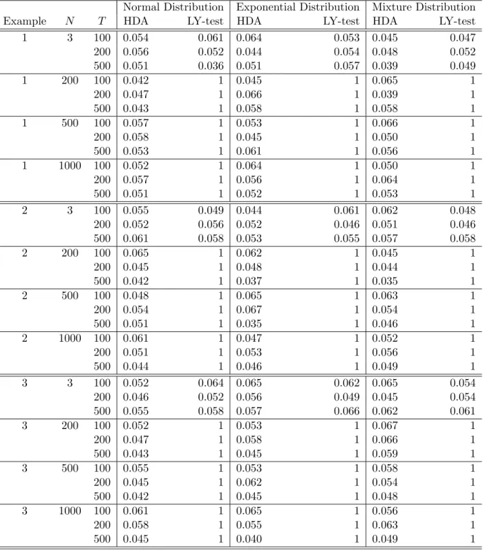
To evaluate the size performance of the HDA test, we set ci = 0 for all i in the above three
examples. Then, three different sample sizes (T = 100,200,500) and four different numbers of stocks (N = 3, 200, 500, 1,000) are considered. For each setting, all simulations are conducted via 1,000 realizations with nominal level α= 5%. The GRS test of Gibbons et al. (1989) and the tests of Pesaran and Yamagata (2012) are only applicable when the factor loadings are constant over time. Hence, we only compare our HDA test with the LY test from Li and Yang (2011).
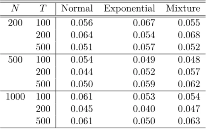
Table 1 presents the sizes of the HDA test across three sample sizes and four different numbers of stocks for Examples 1–3, respectively. Here, the number of interior knots n is determined by the BIC criterion, as discussed in Subsection 2.2, and the order of B-splines is set at 3. The results in Table 1 indicate that HDA performs well regardless of T = 100, 200 or 500, N = 3, 200, 500 or 1,000, and the error distribution being normal, exponential, or a mixture. Hence, HDA is not only applicable to the case N > T, but also robust to various (N, T) specifications and error distributions. It is worth noting that the results of Example 3 yield a similar pattern to those in Examples 1–2. This implies that HDA is also robust to the specification of the factor loadings. In contrast, the LY test exhibits serious size distortion when N is relatively large. For example, the empirical sizes are equal to 1 for
N ≥200. This finding is not surprising since the LY test is not designed for N > T, and it performs well when N = 3. As a result, we only consider HDA in the evaluation of power.
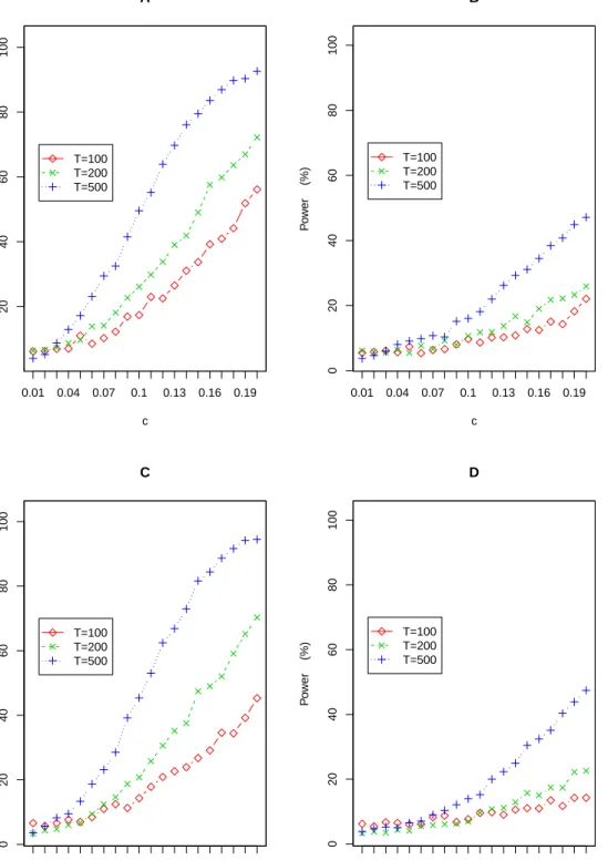
To study the power of the HDA test, we consider the following two different types of alternative hypotheses for Examples 1–2. The first one is the dense alternative under which
αit = cit/T = ct/T for some constant c and i = 1,· · · , N. The second one is the sparse
alternative under whichαit =cit/T =ct/T for some constantcifi≤20; αit = 0, otherwise.
This alternative setting is motivated by the empirical finding of Fan et al. (2015) that the market inefficiency is only induced by a very small portion of stocks. In both alternative settings, the signal strength c ranges from 0 to 0.2 with an increment of 0.01. For the sake of illustration, we only consider the normally distributed random errors withN = 200.
Figures 1 depicts the empirical powers of the HDA test over three sample sizes (T = 100,200,500), two different data generation processes (Examples 1 and 2), two types of alternatives (dense and sparse), and 20 (=0.2/0.01) signals of c. The results indicate that the empirical power of HDA steadily increases to 1 as the signal strength c gets larger. In addition, the power of HDA becomes large as the sample sizeT increases. In sum, the HDA test performs satisfactorily and comparably under both dense and sparse alternatives, and it is indeed consistent.
4.3
Performance of the CC Test
To study the finite sample performance of the CC test, without loss of generality, we consider the case of a single stock (i.e.,N = 1). We adopt the settings given in Examples 1–2, except for βit = 1 +bzt in Example 1 and βijt = 1 +bzt in Example 2 with i = 1. In addition, we
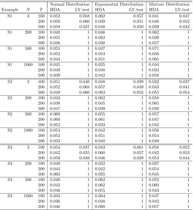
set b = 0 for assessing the size of the test, and b = 0.1 and 0.3 for examining the power of the test. Table 2 reports the test results. From Table 2 we observe that the empirical sizes of the CC test are all around 0.05 regardless of the time lengthT and the error distribution. Furthermore, the empirical power of the CC test increases to 1 asb orT becomes larger. In sum, the CC test performs well in terms of both size and power.
5
Real Data Analysis
In this section, we employ the proposed tests to assess the mean-variance efficiency of both the Chinese and US stock markets. It is worth mentioning that our proposed HDA test is applicable even for N ≫T, which allows us to target a large pool of stocks directly so that there is no need to group a large number of stocks into a small number of portfolios. The goal of this empirical study is two-fold: (i.) investigate the efficiency of the Chinese and US stock markets during the study period; (ii.) explore the differences between the Chinese and US stock markets based on the results of mean-variance efficiency. Since the US stock market is more mature than Chinese stock market, we first study the efficiency of the Chinese stock market and then compare the results with that of the US stock market.
5.1
Data Description
The Chinese stock market data are collected from the WIND database (one of the most authoritative databases in China), which contains securities in the Shanghai-Shenzhen 300 Index. We use this dataset because the 300 stocks in this index are the most frequently traded stocks in China; hence, these data are not significantly impacted by a survivorship bias (see Brown et al., 1995). After eliminating the stocks with missing observations to avoid
analyzing an unbalanced panel, there remain T = 153 weekly observations for each of the
N = 292 stocks from 11/25/2011 to 12/31/2014. As a result, each observation represents a particular firm’s weekly excess return (the stock return minus the risk-free interest rate). The weekly return of the 1-year deposit is chosen to proxy the risk-free interest rate rf t.
Following the literature on the study of the Chinese stock market, we use the Shanghai Composite Index (the value-weighted return on all Shanghai A-share stocks) as the proxy for the market portfolio rmt. Then, according to the definition given by Fama and French
(1993), the factor SMB is the average return of the three smallest portfolios minus the average return on the three biggest portfolios, and the factor HML is the average return on the three highest value stock portfolios minus the average return on the three lowest value portfolios. Note that all the stocks used in this study are listed in the Shanghai and ShenzhenA-share stock market.
To make a comparison with the US stock market, we also collect data for securities in the Standard & Poor’s 500 (S&P 500) index from the period 01/08/2010 to 08/25/2017. After eliminating the assets with missing observations, there remain T = 399 weekly observations for each of the N = 442 firms. The three factors are obtained from Ken French’s data library web page. The one-month US treasury bill rate is chosen as the risk-free rate, and the value-weighted returns on all NYSE, AMEX, and NASDAQ stocks obtained from CRSP are used as a proxy for the market return.
Table 3 reports the descriptive statistics that include the mean, median, and standard deviation (SD) for the market factor, SMB and HML for both the Chinese and US stock markets. According to Table 3, we find that the returns on SMB and HML in the Chinese stock market are much larger than those in the US stock market. It is of interest to note that Aboody and Lev (2000) and Abosede and Oseni (2011), respectively, noticed that SMB and HML can be related to information asymmetry. In addition, Dai et al. (2013) indicated that the Chinese stock market suffers from more information asymmetry, such as insufficient information disclosure mechanisms and regulatory instruments, than stock markets in western countries. Hence, we conjecture that higher information asymmetry in Chinese market maybe leads to the larger observed returns on SMB and HML, but a thorough and rigorous study on this subject needs to be explored in future research and is
not the focus of this paper.
5.2
Are Alphas and Betas Time-Varying?
Before assessing the market efficiency of the Chinese stock market (US stock market), it is reasonable to check whether the alphas and betas are time-varying. To this end, for each individual stock, we employ the CC test to examine the constancy of the alphas and factor loadings in both CAPM and the FF three-factor model. The results show that the p-value for testing the constancy of the alphas and factor loadings in each of the 292 (442) stocks is close to 0, regardless of the model. This strong evidence indicates that the alphas and betas are time-varying in both the Chinese and US stock markets, which suggests that the conditional time-varying factor model is more suitable than the traditional time-invariant factor model.
5.3
Mean-Variance Portfolio Efficiency
We first employ the HDA test to assess the market efficiency of the Chinese stock market based on N = 292 stocks with T = 153 corresponding observations for each stock recorded between 11/25/2011 and 12/31/2014. Specifically, we consider the following rolling window
procedure with window length h = 100 to examine the dynamic movement of the market
efficiency. Due to theoretical considerations,T cannot be too small. Accordingly, the rolling window h cannot be small either. Hence, we consider window length h= 100. For the sake of convenience, we also use h= 100 to study the US stock market.
For each τ ∈ {1,· · · ,153−h}, we separately estimate CAPM and the FF three-factor model using the data from periodτ toτ +h−1. As a result,
rit−rf t = αˆit+ ˆβit(rmt−rf t) + ˆeit (CAP M) ;
rit−rf t = αˆit+ ˆβi1t(rmt−rf t) + ˆβi2tSM Bt+ ˆβi3tHM Lt+ ˆeit (F F)
Based on the estimated residuals ˆeit obtained by separately fitting CAPM and the FF
three-factor model to the data in each window, we calculate the HDA test statistics and their corresponding p-values. Here, the number of interior knots n is determined via BIC discussed in Subsection 2.2, and the order of B-splines is set at 3 for all estimation windows. For the sake of comparison, we also consider the PY test (Pesaran and Yamagata, 2012). The p-values across the 53 (300) windows obtained from the HDA and PY tests by testing the market efficiency of the Chinese (US) stock market based on CAPM and the FF three-factor model are, respectively, presented in Figures 2 and 3, while the descriptive statistics of these p-values are given in Table 4.
For the Chinese market, the left panel in Figure 2 depicts the p-values of the HDA and PY tests for CAPM across the 53 window periods, while the right panel is for FF. According to Figure 2 and Table 4, PY shows a similar pattern to HDA in explaining that the majority of the p-values from FF are larger than those from CAPM. However, these two tests can lead to very different conclusions in terms of market efficiency for some periods under our scrutiny. For example, the left panel in Figure 2 shows that, for 19 window periods (2, 4, 5, 7, 8, 9, 11, 13, 14, 16, 33, 34, 36, 40, 41, 43, 44, 49 and 50), the p-values obtained from HDA in the CAPM model are less than 5%; this indicates that the markets are inefficient over these window periods. In contrast, thep-values obtained from PY in the corresponding window periods are greater than 5%.
We next conduct the analysis for the US stock market data. Panels A and B in Figure 3 depict thep-values of the HDA and PY tests for CAPM and FF, respectively, across the 300 window periods. To highlight the difference between HDA and PY, Panels C and D present the p-values for the sub-window periods ranging from 101 to 150. Table 4 indicates that the averagedp-values obtained from HDA are smaller than those from PY; this can also be seen in Figure 3. In particular, panel D in Figure 3 suggests that, for 8 window periods (108, 110, 111, 112, 134, 135, 149 and 150), the p-values obtained from HDA in the FF model are less than 5%. Accordingly, the markets are inefficient in these window periods. On the other hand, thep-values obtained from PY in those corresponding periods are all greater than 5%. It is also worth noting that the alphas and betas are time-varying, as confirmed by the
CC test in Section 5.2. This, together with the above discussion, implies that HDA is a better and more capable approach than PY to detecting mean-variance inefficiency in these two markets.
In addition to compare HDA and PY, we note from Figures 2 and 3 that most of the
p-values from the FF three-factor model are larger than the 5% significance level, and they are also higher than those from CAPM. Hence, the FF three-factor model is better than CAPM in explaining the mean-variance efficiency of both the Chinese and US stock market. However, in the US stock market these findings are even more prominent than in the Chinese stock market. This suggests that the US stock market is more efficient than the Chinese stock market in terms of mean-variance efficiency. This finding is also confirmed by Table 4; the mean of the p-values from the FF three-factor model obtained for the US stock market is much larger than that for the Chinese stock market.
For robustness check of HDA, we further consider a short window of length h = 60 for both the Chinese and US stock market data as suggested by Pesaran and Yamagata (2012) and a relatively longer window of length h = 200 for the US stock market data; the results yield a similar pattern to that with h = 100. To save space, we present them in the supplementary materials. Finally, although we believe our findings make a contribution to the literature, one avenue of further research would be extending them to account for survival bias when there are missing observations (see Brown et al., 1995).
6
Conclusion
In this paper, we propose the HDA test to examine the market efficiency in conditional time-varying factor models. We also introduce the CC test to assess the constant alphas and factor loadings. Monte Carlo studies demonstrate that both tests perform satisfactorily and the numerical results also support theoretical findings. Moreover, the usefulness of these two tests is illustrated by two empirical examples.