A Probabilistic Approach To Multiple-Instance Learning

(1)

University of Mississippi University of Mississippi

eGrove

Electronic Theses and Dissertations Graduate School

2017

A Probabilistic Approach To Multiple-Instance Learning

Silu Zhang

University of Mississippi

Follow this and additional works at: https://egrove.olemiss.edu/etd Part of the Computer Sciences Commons

Recommended Citation Recommended Citation

Zhang, Silu, "A Probabilistic Approach To Multiple-Instance Learning" (2017). Electronic Theses and Dissertations. 944.

https://egrove.olemiss.edu/etd/944

This Dissertation is brought to you for free and open access by the Graduate School at eGrove. It has been accepted for inclusion in Electronic Theses and Dissertations by an authorized administrator of eGrove. For more information, please contact egrove@olemiss.edu.

(2)

A PROBABILISTIC APPROACH TO MULTIPLE-INSTANCE LEARNING

A Thesis

Presented in Partial Fulfillment of Requirements for the Degree of Master of Science

in the Department of Computer and Information Science The University of Mississippi

by Silu Zhang December 2017

(3)

(4)

ABSTRACT

This study introduced a probabilistic approach to the multiple-instance learning (MIL) problem. In particular, two Bayes classification algorithms were proposed where pos-terior probabilities were estimated under different assumptions. The first algorithm, named Instance-Vote, assumes that the probability of a bag being positive or negative depends upon the percentage of its instances being positive or negative. This probability is estimated using a k-NN classification of instances. In the second approach, Embedded Kernel Density Estimation (EKDE), bags are represented in an instance induced (very high dimensional) space. A parametric stochastic neighbor embedding method is applied to learn a mapping that projects bags into a 2-d or 1-d space. Class conditional probability densities are then estimated in this low dimensional space via kernel density estimation. Both algorithms were evaluated using MUSK benchmark data sets and the results are highly competitive with existing methods.

(5)

TABLE OF CONTENTS ABSTRACT . . . ii LIST OF FIGURES . . . iv LIST OF TABLES . . . v INTRODUCTION . . . 1 METHODOLOGY . . . 5 EXPERIMENTAL RESULTS . . . 9 RELATED WORK . . . 15 DISCUSSIONS . . . 18 CONCLUSIONS . . . 19 BIBLIOGRAPHY . . . 20 VITA . . . 23

(6)

LIST OF FIGURES

3.1 ROC curves obtained by Instance-Vote for (a)MUSK1 and (b)MUSK2. . . 11 3.2 Visualization of (a) MUSK1 and (b) MUSK2 data sets in latent spaces: d= 1

(top) and d = 2 (bottom). Positive and negative bags are colored as red and blue, respectively. . . 12 3.3 Kernel density estimation for d= 1 on (a) MUSK1 and (b) MUSK2. . . 12 3.4 ROC curves obtained by EKDE with d = 1 (top) and d = 2 (bottom) for

(7)

LIST OF TABLES

3.1 Instance-Vote classification accuracy (in %)and AUC with different k. . . 10

3.2 EKDE classification accuracy (in %) and AUC with d= 1 andd= 2 . . . 12

3.3 AUC obtained by the proposed algorithms and other methods on the MUSK data set1_{. . . .} ₁₄

(8)

CHAPTER 1

INTRODUCTION

1.1 Multiple-Instance Learning

In the standard supervised learning, the learner is given a set of training examples where each example is represented as a feature vector and associated with a label. The task is to predict the label of a future example given its feature representation. However, this set-up does not apply when the training examples are grouped into “bags” and the learner only knows whether or not a bag contains a positive example but does not know which one is positive. For example, in the drug activity prediction problem, each drug has more than one conformation with some but not all conformations having the ability to bind to the target. A drug is considered as positive if any of its conformation can bind to the target. As for the training data, only the label for the drug is available, i.e., which conformation that cause a drug to be positive is unknown. Multiple-instance Learning (MIL) is aimed to solve this type of problems. To state the problem in general, a set of grouped examples is called abag, and each example is called aninstance. A bag is considered as positive is any of its instances is positive and negative is none of its instance is negative. The labels in the training set are associated with bags with instance label unknown. The task is to predict the label of an unseen bag based on its instances. In MIL, each instance is represented by a feature vector of a fixed size, while a bag does not necessarily have a feature representation.

MIL has been applied in many scenarios. The first one is drug activity prediction as in the example just given. Each drug is considered as a bag and each conformation is considered as an instance. In this case, only MIL can solve the problem since there is no feature representation for drugs. Another useful application is content-based image retrieval

(9)

and classification. The task is to identify images that contains an object of interest. In this context, each image is considered as a bag and an instance corresponds to a particular region in the image. Although each bag also has a feature representation (i.e., pixels) and can be fitted into a standard supervised learning setting, its performance is not as good as if it is solved by MIL. Some successful cases of MIL in image retrieval are (Maron and Ratan, 1998; Yang and Lozano-Perez, 2000; Zhang et al., 2002). A recent study applied MIL in gene function prediction at the isoform level (Eksi et al., 2013). In this context, a gene can be transcribed into different mRNAs (called isoforms) due to alternative splicing, therefore each gene is referred as a bag and its isoforms are referred as instances. The work is trying to identify which isoform is responsible for the function of its corresponding gene.

1.2 Existing MIL Algorithms

Many MIL algorithms have been proposed (Andrews et al., 2003; Chen et al., 2006; Dietterich et al., 1997; Ray and Craven, 2005; Raykar et al., 2008; Settles et al., 2008; Wang and Zucker, 2000). Notice that the challenge of MIL lies in the fact that, in the training set, the label and feature information does not match, i.e., labels are available only for bags and features are provided only for instances, while a supervised learning algorithms requires both label and feature representation for each training data point. As a result, MIL algorithms usually can be fitted into two categories.

One class of approaches were based upon learning the labels of instances and then labeling the bag using instance label information. The assumption typically used is that a bag is positive if it has at least one positive instance and negative if all of its instances are negative. Dietherich et al. (Dietterich et al., 1997) adapted this assumption to define a axis-parallel rectangle (APR). A bag is positive if one of its instances fall into the APR and negative otherwise. Xu and Frank (Xu and Frank, 2004) used a different assumption that considered all instances equally and independently contribute to a bag’s label. In their algorithm, the bag label was generated by combining the instance-level probability estimates.

(10)

There are also many methods that convert the MIL to a supervised learning problem using a feature mapping. In this way, each bag will have a feature representation. For example, Chen et al. proposed MILES (Multiple-Instance Learning via Embedded Instance Selection) algorithms that maps bags into a instance defined space via bag-instance similarity measurement (Chen et al., 2006). However, feature mapping usually results in increasing in dimensionality. In (Chen et al., 2006), a feature selection method via 1-norm SVM was proposed.

1.3 An Overview of Proposed Approaches

In this study, we developed two Bayes classifiers for MIL. The first approach, named Instance-Vote, predicts a bag label from the predicted labels of instances in the bags. Each instance in the training set is associated with its bag label. To account for the uncertainty introduced by this labeling process, the probability of a bag being positive is estimated by counting instances votes within a bag. A higher number of positive instances in the bag implies a larger chance that the bag is positive. For any new bag, we first use a k-NN classifier to predict the label for each instance in the bag, followed by estimating the probability of the bag being positive via the percentage of the positive instances in the bag.

The second algorithm, named as EKDE (Embedded Kernel Density Estimation) con-verts the MIL to a supervised learning by mapping each bag into a instance-defined space. A parametric nonlinear dimensionality reduction (DR) method, t-SNE (t-Distributed Stochas-tic Neighbor Embedding), is then used to reduce the dimension to 1 or 2 (Note that this also provides a visualization of the data.) Next, the class conditional probability densities are estimated in this low dimensional space by kernel density estimation. Finally, the posterior probability of bag being positive is estimated based on Bayes’ theorem.

The proposed algorithms have the following advantages:

• The Instance-Vote algorithm has an extremely simple model with competitive perfor-mance.

(11)

• The EKDE algorithm has the ability to visualize the data, which provides a better understanding of the data.

The rest of the thesis is organized as follows: Chapter 2 gives the detailed descriptions on each algorithm; Chapter 3 shows the experimental results on MUSK1 and MUSK2 dataset; Chapter 4 summarizes the related work that our MIL algorithms are inspired from; Chapter 5 expands some discussions on the proposed algorithms; Chapter 6 concludes this work.

(12)

CHAPTER 2

METHODOLOGY

2.1 MIL via Instance-Vote

2.1.1 A New Interpolation of Instance Label

The main challenge of MIL is that the label of instances are unknown. The classical MIL assumption describes that a bag is positive if any of its instances is positive and neg-ative otherwise. Here we relax the assumption by allowing negneg-ative bag to contain positive instances. In addition, we assume that the prediction of a bag depends on the probability of observing a positive (or negative) instance within the bag.

In order to predict instance labels, we assign bag label to all its instances in the training set. We then use k-NN classifier to predict instance labels. This above process of generating instance-based training data clearly introduces noise into instance labels. How-ever, the noise can be accounted by the following voting model and the choice of threshold parameter.

2.1.2 Voting for Bag Label

To classify a bag, all its instances cast a vote based on the instance label. We assume that the posterior probability of a bag being positive (or negative) is a monotonically non-decreasing function of the probability of a randomly chosen instance from the bag being positive (or negative), i.e.,

(13)

whereyis the label of bagB,xiis a randomly chosen instance from the bag,f is an unknown

monotonically non-decreasing function. The maximum likelihood estimate of Pr(xi ∈+|B)

is obtained as

Pr(xi ∈+|B) =

m+

m

where m+ _{is the number of positive instances in the bag and} _m _{is the total number of}

instances in the bag.

We use a simple Bayes decision rule which states that bag B is positive if

Pr(y= +|B)>Pr(y=−|B).

Asf is a monotonically non-decreasing function, the above decision rule is equivalent to the

following decision rule:

y=        + if Pr(xi ∈+|B)> θ, − otherwise, (2.1)

for some unknown value of θ, which can determined by cross validation.

2.2 Embedded Kernel Density Estimation

In this approach, we convert MIL problem to supervised learning via feature mapping. We aim to find the probability distributions of positive and negative bags using kernel density estimation and then apply the Bayes decision rule. However, kernel density estimation does not perform well for high dimensional data, since data points are too sparse in high dimensional space. To overcome the problem, we first learn an embedding of the data in a low dimensional latent space (d = 1 or 2) and then apply kernel density estimation in the

latent space. Therefore, we name this approach as Embedded Kernel Density Estimation (EKDE).

(14)

2.2.1 Feature Mapping

We adopt the same method described in Chen et al. (2006) considering its good performance. Each bag is represented by all the instances in the training set via a similarity measurement. The similarity of a bag Bi and an instance xk (the superscript k is used to

represent an instance from the training set, not necessarily from the bagBi) is defined as:

s(Bi, xk) = max j exp(− xij −xk 2 σ2 )

wherexij is thej’th instance in bagBi withj = 1, ..., ni andσ is a predefined scaling factor.

Then bag Bi can be represented as:

[s(Bi, x1), s(Bi, x2), ...s(Bi, xn)]

where n is the total number of instances in the training set. The dimension after feature

mapping is nown, which can be considerably large. Therefore, DR is desired.

2.2.2 Dimensionality Reduction and Visualization

Among all existing DR techniques, a non-linear method t-SNE(t-Distributed Stochas-tic Neighbor Embedding) was chosen due to its prominent performance on visualization Maaten and Hinton (2008). Specifically, we chose the parametric t-SNE since it provides a mapping function from the original space to the low dimensional spacevan der Maaten (2009).

The mapping is learned by training a feed-forward neural network. The dimension was reduced to 1 or 2 such that kernel density estimation can be reliably implemented. Visualization of the data can also be performed at this stage. Although not required by classification, visualization is beneficial for a better understanding of high dimensional data.

(15)

2.2.3 Kernel Density Estimation and Classification

According to Bayes’ theorem, given a bag represented asx, the posterior probabilities

can be computed as

Pr(y= +|x) = p(x|y= +) Pr(y= +)

p(x) ,

Pr(y=−|x) = p(x|y=−) Pr(y =−)

p(x)

where y is the bag label. Assuming bags being i.i.d. , the maximum likelihood estimates of

Pr(y= +) and Pr(y=−) are Pr(y= +) = l + l , Pr(y=−) = l − l

where l+₍_l−_{) is the number of positive(negative) bags in trainning set, and} _l _{is the total}

number of bags in the training set. The class conditional densities p(x|y = +) and p(x|y=

+) can be estimated by kernel density estimation using training data after dimensionality reduction. Then the odd ratio (OR) can be computed as

OR = Pr(y= +|x) Pr(y =−|x) =

p(x|y= +) Pr(y= +)

p(x|y=−) Pr(y=−).

The classifier can make prediction on the bag label y by setting a threshold θ for the odd

ratio (θ= 1 corresponding to the Bayes decision under the estimated posterior):

y=        + if OR> θ, − otherwise. (2.2)

(16)

CHAPTER 3

EXPERIMENTAL RESULTS

3.1 Data Sets

The benchmark datasets MUSK1 and MUSK2 are used in our study. Both datasets are publicly available from UCI Machine Learning Repository (UCI). In these two datasets, each molecule (bag) has more than two conformations (instances). The label of the molecule is “musk” (positive) if any of its conformation is a musk or “non-musk” if none of its confor-mation is a musk. Each conforconfor-mation is represented by 166 features. In MUSK1, there are total 92 molecules with 47 of them labeled as musk and the rest labeled as non-musk. The total number of conformations in MUSK1 is 476. In MUSK2, there are total 102 molecules with 39 of them labeled as musk and the rest labeled as non-musk. The total number of conformations in MUSK2 is 6598.

3.2 Experimental Setup

For the Instance-Vote algorithm, different values of k was tested for k-NN classifier

in instance classification. A default threshold θ= 0.5 was used for bag classification.

For EKDE algorithm, the variance σ2 used in feature mapping was set to 5×104

and 8×104 for MUSK1 and MUSK2, repectively, according to Chen et al. (2006). We used the implementation of parametric t-SNE that is publicly available at Matten. Note that the implementation requires the data input to be normalized. Since the feature mapping in our method yields values between 0 and 1, no further data processing is required. Parameters used in parametric t-SNE are: perplexity = 30, layers = [500 500 2000d] (whered= 1 or 2),

(17)

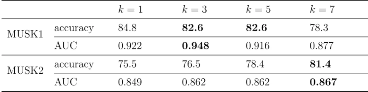
Table 3.1. Instance-Vote classification accuracy (in %)and AUC with different k. k = 1 k = 3 k = 5 k = 7 MUSK1 accuracy 84.8 82.6 82.6 78.3 AUC 0.922 0.948 0.916 0.877 MUSK2 accuracy 75.5 76.5 78.4 81.4 AUC 0.849 0.862 0.862 0.867

kernel was used and the optimal bandwidth was determined by 20-fold cross validation. A default threshold θ = 1 was set for classification.

3.3 Experimental Results

To evaluate the Instance-Vote algorithm, leave-one-out tests were performed at the bag level, i.e., a whole bag of instance were held out for testing. Both classification accuracy and receiver operating characteristic (ROC) curve were used for evaluation. The ROC curve was obtained by varying the threshold θ in equation (2.1) from 1 to 0. The ROC curve was

plotted by pooling all the validation results.

Table 3.1 shows the classification accuracy and area under ROC curve (AUC) for different values of k. The best results are bolded. ROC curves with best AUC, i.e., k = 3

for MUSK1 and k = 7 for MUSK2, are shown in Fig. 3.1. The classification accuracy was

obtained by using a default threshold, i.e., θ = 0.5. However, the ROC curve suggests

that a better classification accuracy could be obtained if the a higher value was chosen for

θ. Specifically, the accuracy for MUSK1 and MUSK2 would be 89.1% and 85.3% if the

correspondingθ was set to 0.75 and 0.71, respectively. This suggests that negative instances

should be given more weights in the vote. It can be explained by the existence of “false positive” instances that should not contribute to the bag label. Similar observation was also presented by Wang Wang and Zucker (2000). Therefore, a potential improvement on the classifier is to optimize the threshold θ via cross validation.

(18)

0.0 0.2 0.4 0.6 0.8 1.0 False Positive Rate

0.0 0.2 0.4 0.6 0.8 1.0 Tr ue P osi ti ve R at e MUSK1 (AUC = 0.948) 0.0 0.2 0.4 0.6 0.8 1.0 False Positive Rate

0.0 0.2 0.4 0.6 0.8 1.0 Tr ue P osi ti ve R at e MUSK2 (AUC = 0.867) (a) (b)

Figure 3.1. ROC curves obtained by Instance-Vote for (a)MUSK1 and (b)MUSK2.

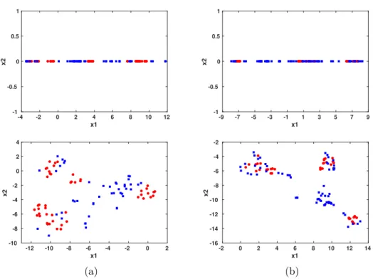
feature mapping, the dimension of the data is 476 for MUSK1 and 6598 for MUSK2, as determined by the total number of instances in the training sets. The dimension is then reduced to 1 or 2 by applying parametric t-SNE. Thus, the embedding of the data can be visualized as shown in Fig. 3.2. The positive bags (MUSK molecules) are shown as red circles and the negative bags (Non-MUSK molecules) are shown as blue squares. The results are satisfying even in 1D, thanks to the superiority of t-SNE on preserving the local structure. We can see that the two classes are separated well for both data sets with minor overlapping in MUSK2. Then a kernel density estimation was performed for both d = 1 and d = 2.

The plots for d = 2 are in 3D, therefore we only show those obtained for d = 1 (Fig. 3.3).

Same colors were used to denote positive and negative bags as in Fig. 3.2. It is clear to see that each class peak at different locations. Finally, the classification results are shown in Table 3.2. Best AUCs were obtained with d = 2 and best classification accuracy were

obtained with d = 1. We also present the ROC curves in Fig. 3.4. The ROC curves were

generated by setting the threshold θ(in equation (2.2)) from ∞ to 0. The ROC curves

of the EKDE algorithm also suggest that a better threshold θ could be used to improve

(19)

-4 -2 0 2 4 6 8 10 12 x1 -1 -0.5 0 0.5 1 x2 -9 -7 -5 -3 -1 1 3 5 7 9 x1 -1 -0.5 0 0.5 1 x2 -12 -10 -8 -6 -4 -2 0 2 x1 -10 -8 -6 -4 -2 0 2 4 x2 -2 0 2 4 6 8 10 12 14 x1 -16 -14 -12 -10 -8 -6 -4 -2 x2 (a) (b)

Figure 3.2. Visualization of (a) MUSK1 and (b) MUSK2 data sets in latent spaces: d

= 1 (top) and d = 2 (bottom). Positive and negative bags are colored as red and blue, respectively. −4 −2 0 2 4 6 8 10 12 x 0.00 0.05 0.10 0.15 0.20 0.25 0.30 0.35 0.40 0.45 p( x| y) positive negative −8 −6 −4 −2 0 2 4 6 8 10 x 0.00 0.05 0.10 0.15 0.20 0.25 0.30 0.35 0.40 p( x| y) positive negative (a) (b)

Figure 3.3. Kernel density estimation for d= 1 on (a) MUSK1 and (b) MUSK2.

Table 3.2. EKDE classification accuracy (in %) and AUC with d= 1 andd= 2

d= 1 d = 2

MUSK1 accuracy 90.2 88.0

AUC 0.969 0.972

MUSK2 accuracy 82.4 80.4

(20)

0.0 0.2 0.4 0.6 0.8 1.0 False Positive Rate

0.0 0.2 0.4 0.6 0.8 1.0 Tr ue P osi ti ve R at e MUSK2 (AUC = 0.886) (a) (b)

Figure 3.4. ROC curves obtained by EKDE withd = 1 (top) andd= 2 (bottom) for MUSK1 (a) and MUSK2 (b) data sets.

(21)

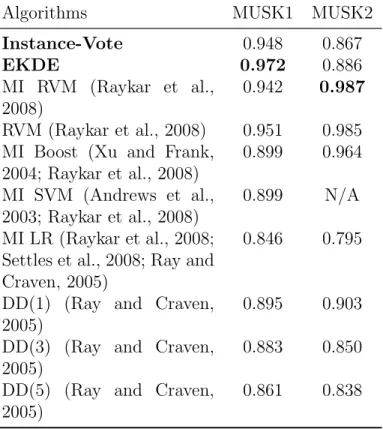
Table 3.3. AUC obtained by the proposed algorithms and other methods on the MUSK data set1_.

Algorithms MUSK1 MUSK2

Instance-Vote 0.948 0.867 EKDE 0.972 0.886 MI RVM (Raykar et al., 2008) 0.942 0.987 RVM (Raykar et al., 2008) 0.951 0.985 MI Boost (Xu and Frank,

2004; Raykar et al., 2008) 0.899 0.964 MI SVM (Andrews et al., 2003; Raykar et al., 2008) 0.899 N/A MI LR (Raykar et al., 2008; Settles et al., 2008; Ray and Craven, 2005)

0.846 0.795

DD(1) (Ray and Craven, 2005)

0.895 0.903 DD(3) (Ray and Craven,

2005)

0.883 0.850 DD(5) (Ray and Craven,

2005)

0.861 0.838

3.4 Comparison with Other Algorithms

The proposed two algorithms (bolded) are compared with other methods in terms of AUC, as shown in Table 3.3. The best AUCs are bolded for MUSK1 and MUSK2. Among all the listed method, Instance-Vote is the simplest and has comparable results with others. This indicates the rationality of the new interpolation of the instance label. The EKDE algorithm outperforms others on MUSK1 and is comparable with other methods on MUSK2.

1_{The proposed algorithms were evaluated by the leave-one-out test while others were based on tenfold}

(22)

CHAPTER 4 RELATED WORK 4.1 From Instance Label to Bag Label

The original assumption of MIL is that a bag is positive if it contains at least one positive instance and negative if no positive instance exits in the bag. Considering the lack of label information at the instances level, this assumption may be too strict to solve the problem. Some researchers such as Xu and Frank (Xu and Frank, 2004) modified the assumption by assuming all instances equally and independently contribute to a bag’s label, which allows negative bags to have positive instances. They proposed two ways to relate instance-level class probability Pr(y|xi) and bag-level class probability Pr(Y|b), specified as

respectively. The interpretation of the above equations is that the bag-level class probability is the arithmetic mean of instance-level probability in (4.1) and geometric mean in (4.2). Our Instance-Vote algorithm is actually a special case of the former, where the instance-level probability Pr(y|xi) is either 1 or 0. However, the performance of our simplified approach is

(23)

4.2 Feature Mapping

The propose of feature mapping is to find a feature representation for bags. We used the same feature mapping method proposed by Chen et al. (Chen et al., 2006). The advantage of this feature mapping is that it does not require or attempt to learn the label information at the instance-level. It uses a similarity measurement to define a bag using all instances in the training data. This seems to be a problem when the training set is large. However, with proper dimensionality techniques, the overall performance is in the leading place among all MIL algorithms.

Note that there are also alternative ways to predict bag label without knowing in-stance label and bag representation. When a k-NN classifier is used, the feature representa-tion of bags is not necessarily needed, as long as the neighborhood informarepresenta-tion is defines, as in the case of Bayesian-kNN and Citation-kNN, where Hausdroff distance is used to define the distance between bags (Wang and Zucker, 2000). However, an explicit feature representation for bags is more general and can be fitted in any supervised model.

4.3 Dimensionality Reduction

A crucial part of the EKDE algorithm is DR, which enables the following KDE to be effective. Although any DR technique can be used, there are some reasons that we chose t-SNE. A key requirement is that the algorithm should be able to learn a explicit mapping function from the original space to the latent space in order to be applied to a classification problem for the sake of efficiency. If the mapping function is unknown, every time to predict a new example, it first need to be added to the existing data and then recompute the mapping in order to get the coordinates of the new example in the low dimensional space. With a learned mapping function, however, the coordinates of a new data point can be calculated easily from the mapping function. Among all existing DR algorithms, t-SNE has the leading performance on most of the tasks as well as a parametric version that is able to learn a mapping function (Maaten and Hinton, 2008; van der Maaten, 2009).

(24)

There are two key features that t-SNE differs other DR algorithms. The first is the objective function, which measures the difference in the distribution of pairwise similarity between the original space and learned latent space. The t-SNE objective function is

C =KL(P||Q) = X i6=j pijlog pij qij ,

where pij and qij are the pairwise similarity in the original space and the latent space,

re-spectively. Another unique feature in t-SNE is that it uses different distribution to measure pairwise similarity in different spaces. In specific, pij is measured using a Gaussian

distri-bution and qij is measured by a Student t-distribution. According to the author, by using

different distribution, t-SNE is able to solve the “crowding problem”, i.e., there is not enough space in the low-dimensional map to accommodate moderately distant data points, which is the main challenge in DR. The unique measurement of pairwise similarity combined with the t-SNE cost function is very likely the main factor that makes t-SNE so successful and widely used.

(25)

CHAPTER 5

DISCUSSIONS

We have shown that the Instance-Vote algorithm is very simple and has competitive performance on the MUSK data sets. However, its weakness is that the performance is very data dependent. Recall in the instance labeling process, noises are introduced. In an extreme case, if the true labels of instances in positive bags are all positive, there will be no incorrectness at all in the labeling process and we would expect this approach to be very successful. In the other extreme, if there is only one positive instance in each positive bag, the noises introduced would be too big to make this approach effective. Therefore some knowledge on the expected number of positive instances in a positive bag would be very helpful on selecting an appropriate MIL algorithm.

As for the EKDE algorithm, it is very attracting to have the capability of data visualization, but the performance is not guaranteed to be better than using features in its original space. Usually the prediction performance will drop as feature dimension is reduced, which is the main reason that t-SNE is more applied in pure data visualization than classification. However, there is always a trade-off between classification accuracy and model simplicity. Anther issue of applying t-SNE in a classification algorithm is the computational cost. The bottle neck of t-SNE is the calculation of pairwise similarities, which requires

O(n2_{) time, where} _n _{is the number of training data points. It is acceptable for relative}

small data sets but does not scale to millions of data points. For pure visualization, it is reasonable and acceptable to approximate the mapping by using a sample of the data, however, a classification algorithm is supposed to use all available training data.

(26)

CHAPTER 6

CONCLUSIONS

In this study, we introduced two algorithms to solve the multiple-instance problem, named as Instance-Vote and EKDE, respectively. The Instance-Vote algorithm departs from existing methods by attaching the bag label to its instances with a new interpolation: a in-stance is positive if it belongs to a positive bag and negative otherwise. This converts inin-stance learning to standard supervised learning and the bag label is determined by the percentage of positive instances it contains. The second algorithm, EKDE, solves the multiple-instance problem by feature mapping. The kernel density estimation is performed in the embedded low dimensional space with the help of parametric t-SNE, a non-linear dimensionality reduc-tion technique aimed at preserving local structure. In this approach, both classificareduc-tion and data visualization can be achieved. We have shown that both algorithms are competitive with other MIL algorithms on benchmark data sets MUSK1 and MUSK2.

(27)

(28)

BIBLIOGRAPHY

(), Uci machine learning repository: Data sets.

Andrews, S., I. Tsochantaridis, and T. Hofmann (2003), Support vector machines for multiple-instance learning, Advances in neural information processing systems, pp. 577– 584.

Chen, Y., J. Bi, and J. Z. Wang (2006), Miles: Multiple-instance learning via embedded in-stance selection,IEEE Transactions on Pattern Analysis and Machine Intelligence, 28(12), 1931–1947.

Dietterich, T. G., R. H. Lathrop, and T. Lozano-P´erez (1997), Solving the multiple instance problem with axis-parallel rectangles, Artificial intelligence, 89(1), 31–71.

Eksi, R., H.-D. Li, R. Menon, Y. Wen, G. S. Omenn, M. Kretzler, and Y. Guan (2013), Sys-tematically differentiating functions for alternatively spliced isoforms through integrating rna-seq data,PLoS computational biology, 9(11), e1003,314.

Maaten, L. v. d., and G. Hinton (2008), Visualizing data using t-sne, Journal of Machine

Learning Research, 9(Nov), 2579–2605.

Maron, O., and A. L. Ratan (1998), Multiple-instance learning for natural scene classifica-tion., in ICML, vol. 98, pp. 341–349.

Matten, L. (), t-sne.

Ray, S., and M. Craven (2005), Supervised versus multiple instance learning: An empirical comparison, inProceedings of the 22nd international conference on Machine learning, pp. 697–704, ACM.

Raykar, V. C., B. Krishnapuram, J. Bi, M. Dundar, and R. B. Rao (2008), Bayesian multiple instance learning: automatic feature selection and inductive transfer, inProceedings of the

25th international conference on Machine learning, pp. 808–815, ACM.

Settles, B., M. Craven, and S. Ray (2008), Multiple-instance active learning, inAdvances in

neural information processing systems, pp. 1289–1296.

van der Maaten, L. (2009), Learning a parametric embedding by preserving local structure,

RBM, 500(500), 26.

Wang, J., and J.-D. Zucker (2000), Solving multiple-instance problem: A lazy learning approach.

(29)

Xu, X., and E. Frank (2004), Logistic regression and boosting for labeled bags of instances,

inPacific-Asia conference on knowledge discovery and data mining, pp. 272–281, Springer.

Yang, C., and T. Lozano-Perez (2000), Image database retrieval with multiple-instance learn-ing techniques, inData Engineering, 2000. Proceedings. 16th International Conference on, pp. 233–243, IEEE.

Zhang, Q., S. A. Goldman, W. Yu, and J. E. Fritts (2002), Content-based image retrieval using multiple-instance learning, inICML, vol. 2, pp. 682–689.

(30)

VITA

Education

B.S. Bioengineering, Zhejiang Univerisity, China, 2011.

M.S. Chemical Engineering, North Carolina State University, 2011.

Employment

Research Assistant, North Carolina State University, 2011–2013. Research Assistant, University of Texas at Dallas, 2013–2015. IT Intern, Fedex Service, 2017

Teaching Assistant, University of Mississippi, Current.

Publications

Khan, M. R., Hayes, G. J., Zhang, S., Dickey, M. D., & Lazzi, G. (2012). A pres-sure responsive fluidic microstrip open stub resonator using a liquid metal alloy. IEEE Microwave and Wireless Components Letters, 22(11), 577-579.

Zhang, S., Zang, P., Liang, Y., & Hu, W. (2014, August). Determination of protein titration curves using Si Nanograting FETs. In Nanotechnology (IEEE-NANO), 2014 IEEE 14th International Conference on (pp. 934-938). IEEE.

Zang, P., Zhang, S., Liang, Y., & Hu, W. (2014, August). Noise suppression with ad-ditional reference electrode for time-dependent protein sensing tests with Si nanograting FETs. In Nanotechnology (IEEE-NANO), 2014 IEEE 14th International Conference on (pp. 930-933). IEEE.

Liang, Y., Zhang, S., & Hu, W. (2015, September). Detection of base pair charges during DNA extension with Si nanowire FETs towards DNA sequencing. In Nanotechnology Materials and Devices Conference (NMDC), 2015 IEEE (pp. 1-2). IEEE.

(31)

Zhang, S., Chen, Y., & Wilkins, D. (2017, May). A Probabilistic Approach to Multiple-Instance Learning. In International Symposium on Bioinformatics Research and Appli-cations (pp. 331-336). Springer, Cham.