CONSUMER-DRIVEN OPERATIONS: EMPIRICAL
AND EXPERIMENTAL STUDIES IN DEMAND
MODELS
A Dissertation
Presented to the Faculty of the Graduate School of Cornell University
in Partial Fulfillment of the Requirements for the Degree of Doctor of Philosophy
by Dayoung Kim
c
2017 Dayoung Kim ALL RIGHTS RESERVED
CONSUMER-DRIVEN OPERATIONS: EMPIRICAL AND EXPERIMENTAL STUDIES IN DEMAND MODELS
Dayoung Kim, Ph.D. Cornell University 2017
The new selling techniques enabled by information technologies in today’s market-places, such as online sales channels, search portals, and review platforms, changed the consumer-driven demand in many ways. Unlike traditional retail competition, mostly driven by product attributes (e.g., quality, price, etc.), these selling techniques based on information technologies have become more important to consider customer behav-ior and its resulting effect in shaping demand, in order for firms to better plan their operational strategies. In this dissertation, we investigate different sources of demand uncertainty and obtain insights into operations of the firms competing in the current marketplace. We develop methods for more accurate estimations of demand in the pres-ence of downstream customers’ choice behavior or social interactions. We adopt the Markov Chain based model to understand customer demand and validate the model us-ing human-subject experiment and field data. We also conduct empirical research to capture online browsing behavior of consumers and provide implications to operational managers.
This dissertation consists of three chapters.
- Chapter 1: The Effect of Social Information on Demand in Quality Competition. This is joint work with Professor Vishal Gaur and Professor Andrew Davis - Chapters 2: Predicting Order Variability in Inventory Decisions: A Model of
Fore-cast Anchoring. This is joint work with Professor Andrew Davis and Professor Li Chen
- Chapter 3: Predicting Purchase Propensity from Online Browsing Behavior. This is joint work with Professor Vishal Gaur
The three chapters are self-contained but are related to one another: Chapter 1 investi-gates the impact of social information on demand uncertainty using experimental work, Chapter 2 explores the sources of amplified demand uncertainty from the downstream buyers’ inventory decisions, and Chapter 3 empirically explores the effect of online browsing behavior on demand prediction and is a work-in-progress. All these chap-ters commonly focus on the behavioral sources of demand endogeneity. Therefore, this dissertation aims to contribute to improve the accuracy of demand estimation by incor-porating those behavioral factors into the models in Operations.
BIOGRAPHICAL SKETCH
Dayoung Kim received a Bachelor’s degree in Business Administration and Master’s degree in Management Science, from Seoul National University. She received her Mas-ter’s and doctoral degree in Operations, Technology and Information Management from SC Johnson College of Business at Cornell University.
ACKNOWLEDGEMENTS
The completion of this dissertation would not have been possible without the support of a number of people throughout this monumental journey. I would first like to express my sincere gratitude to my adviser, Professor Vishal Gaur. His enthusiastic guidance helped shape my identity as a scholar, and his profound insights always made me feel humbled and inspired. It has been a privilege to work with him. I owe my gratitude to amazing committee members as well. I have been extremely fortunate to meet Professor Andrew Davis, a great mentor who has provided me with continuous support and hands-on help. With his attentive guidance, I was able to develop my interest and expertise in behavioral operations. My sincere gratitude goes to Professor Nagesh Gavirneni for his warm encouragement which has been invaluable on both academic and personal level. I am very grateful to Professor Li Chen for his academic guidance and encouragements in many aspects. I would like to thank Professor William Schmidt, Yao Cui, and Lawrence Robinson for their constructive feedback throughout my years of doctoral training that helped me grow as a researcher.
The time I spent at Cornell made me realize how important it is to stay courageous and positive. I feel very fortunate to have met lifelong mentors and friends. Heartfelt thanks go to my fellow sufferers - Junhyun, Xiaobo, Meredith, Xiaoyan, and Zhen - for their comradeship and empathy. I also would like to thank my dearest friends, Lawrence et al., for believing in me and making me laugh even during the hardest times. Last but not least, none of this incredible journey would have been possible if it were not for my family’s endless love and unconditional support. Their love is what keeps me going.
TABLE OF CONTENTS
Biographical Sketch . . . iii
Dedication . . . iv
Acknowledgements . . . v
Table of Contents . . . vi
List of Tables . . . viii
List of Figures . . . ix
1 The Effect of Social Information on Demand in Quality Competition 1 1.1 Introduction . . . 1 1.2 Model . . . 6 1.2.1 Model Description . . . 6 1.2.2 Hypotheses . . . 17 1.2.3 Parameter Estimation . . . 19 1.3 Experimental Design . . . 20 1.4 Results . . . 23 1.4.1 Parameter Estimation . . . 23 1.4.2 Market Share . . . 26 1.4.3 Demand Uncertainty . . . 30 1.4.4 Convergence Speed . . . 34 1.5 Robustness Checks . . . 36
1.5.1 Supporting Alternative Logit Model . . . 36
1.5.2 Treatment with Both Types of Social Information . . . 38
1.6 Conclusion . . . 40
1.7 Appendices . . . 43
1.7.1 Technical Details in Bayesian and WSLS Benchmark . . . 43
1.7.2 Technical Details on Convergence Speed Test . . . 47
2 Predicting Order Variability in Inventory Decisions: A Model of Forecast Anchoring 51 2.1 Introduction . . . 51
2.2 Literature Review . . . 55
2.3 Forecast Anchoring Model . . . 59
2.4 Model Estimation and Validation . . . 62
2.4.1 Parameter Estimation . . . 62
2.4.2 Cross-Study Out-of-Sample Validation . . . 65
2.4.3 Individual Heterogeneity . . . 69
2.5 Conclusion . . . 71
3 Predicting Purchase Propensity from Online Browsing Behavior 74 3.1 Introduction . . . 74
3.2 Data Description . . . 79
3.4 Implication in Operations . . . 88 3.5 Conclusion . . . 89
LIST OF TABLES
1.1 Two parameter model estimates . . . 24
1.2 Four parameter model estimates . . . 25
1.3 Prediction error in the hold-out samples (period 31-40) . . . 26
1.4 Market share of the High-firm under different SI treatments . . . 28
1.5 Average satisfaction rates of all subjects in each treatment, and the sub-jects visiting each firms . . . 29
1.6 Percentage of time switching and expected sojourn time over 40 periods 32 1.7 Stationary probability (π) of the belief transition matrixPand the con-vergence speed measures . . . 34
1.8 Logit regression on the choice of the High-firm by each treatment . . . 37
1.9 Average of subjects’ elicited estimate of service quality (%) for the High and Low-firm . . . 39
1.10 SI promotion strategy recommended to the firms with different quality in competition . . . 42
2.1 Estimated Parameters and Prediction Results for the BK Data . . . 64
2.2 Estimated Parameters of FA Model from Pooled OS Data using the OS Estimates . . . 68
3.1 Summary statistics of the purchase data from three companies . . . 80
3.2 Summary Statistics of the sessions . . . 81
3.3 Length of Active Engagement . . . 82
3.4 User- and Session- level Logit Regression on the Conversion . . . 84
LIST OF FIGURES
1.1 Transition diagram: transitions between the hidden belief states and the visit probability . . . 12 1.2 Transition diagram between the 8 states ofM(S). . . 12 1.3 Preliminary simulation result: Expected market share and the variance
of High-firm with respect to the weight on recency biasα . . . 15 1.4 Preliminary simulation result: Expected market share and the variance
of High-firm with respect to the own learning propensityh . . . 15 1.5 Demand uncertainty under different types of SI (standard deviation)
under Large-gap (left) and Small-gap (right) treatment . . . 31 1.6 Percentage of frequent switchers and loyal consumers under different
SI treatments . . . 33 1.7 Bootstrapped probability distribution of second-largest eigenvalues of
estimated transition matrices: Solid lines are from the transition ma-trices estimated using the first 15 periods, dashed lines are from the transition matrices estimated using the latter 25 periods. . . 49 2.1 Observations from BK and Predictions by the Forecast Anchoring (FA)
and Bounded Rationality (BR) Models . . . 66 2.2 Cross-Study Out-of-Sample Validation: Mean (left) and Variability
(right) Fit of OS Data using the BK Estimates . . . 67 2.3 Within-Study Validation of the Estimates: Mean (left) and Variability
(right) Fit of OS Data . . . 68 2.4 Scatter Plots of Estimates: Subject-LevelλandσΛDistribution of BK
(left) and OS (right) data . . . 70 3.1 CDF of Time Between Clicks . . . 83 3.2 The Number of Repeated Buyers . . . 86
CHAPTER 1
THE EFFECT OF SOCIAL INFORMATION ON DEMAND IN QUALITY COMPETITION
1.1
Introduction
In the services industry where a firm’s true quality is not explicitly known to consumers, social information generated through the interaction of people plays a critical role in determining which firm to visit. Often times, this social information is depicted to consumers in different ways. For instance, Urbanspoon.com lists the ‘most popular’ restaurants in town, whereasZocdoc.comdisplays doctors according to ‘quality ratings’ by patients. In these examples, the overall popularity rankings and number of reviews contain market share-based information reflecting the choices of consumers, whereas the average product ratings and reviews contain quality-based information. This raises the question as to whether consumers respond differently to various aspects of social information, affecting a firms’ demand characteristics in alternative ways. If so, it is im-portant that firms understand these differing impacts on demand so that they can make better operational and planning decisions. Furthermore, it may also help a firm deter-mine whether they should strategically choose which type of information to promote to their customers through their own social media outlets. In this study, we investigate the effects of different types of social information on consumers’ choice between firms, and their resulting impact on the firms’ market shares and demand uncertainties.
Empirical evidence suggests that social information plays a significant role in how consumers choose among firms. For example, periodic surveys conducted by Nielsen illustrate that consumers consider earned recommendations from friends and family as the most trustworthy source of information followed by information posted on
brand-managed (owned) websites and consumer opinions posted online as the most reliable source of information [55]. Additionally, a growing academic literature demonstrates that humans, when making decisions, learn and are influenced by information in dif-ferent ways (e.g. [30, 16]). Thus, it is important for firms to understand the effect that social information has on consumers’ choices for visiting firms, and how this then af-fects their demand characteristics for better operational decision making. However, in practice, it is difficult for firms to make this assessment for two reasons: (i) they often have access to only partial data, i.e., visits by customers to their stores, but not the visits to competitors’ stores, and (ii) customers are presented with more than one type of social information simultaneously, so that their effects are difficult to disentangle. This chapter addresses this problem by conducting a controlled laboratory experiment in which dif-ferent types of social information are presented to different treatment groups of subjects and their subsequent choice behavior is analyzed.
In the operations management literature, there has been recent work on the role of social information and its impact on consumers’ choices (e.g. [74], [58], [39], and [69]). Additionally, fields such as economics and marketing have incorporated social learning into consumer choice models ([27, 5, 3]). The marketing literature collectively identifies the key dimensions of social communication that determine the effectiveness of social information as the source, the volume, and the valence: the source of information indi-cates where the information is coming from, the volume of information indiindi-cates how much information on the firm is available, and the valence indicates positivity or nega-tivity of the contents delivered through social information. However, much of this work neglects to distinguish between different characteristics of firms disclosed by social in-formation, such as the number of reviews for a firm versus the average quality rating of a firm.1 Of the few select works that are an exception to this, Park et al. [60] take a
1Some papers in marketing distinguish between the volume of social information and consumers’ observational learning on others’ choices. We consider that both the volume of information and the
theoretical approach to investigating the impact of different types of social information on demand. They find that the market share of competing firms can change when a consumer’s recency bias interacts with her weight on different types of social informa-tion. From an empirical standpoint, Chen et al. [22] investigate the effect of two types of social information using data fromAmazon.com. Some other studies exhibit conflict-ing evidence on how the different types of information influence the performance of the firms, e.g., [33, 23] and [47]. We contributes to this literature by developing a behavioral Hidden Markov chain model of consumer choice and conducting a controlled human-subject experiment that permits us to tease out the effect of two common, but different, types of social information on consumers’ choices. Markov-chain based choice models have been used recently in the revenue management problems when consumers make choices from product assortments [11]. A Hidden Markov Model (HMM) has also been used by [2] in modeling of individual consumer behavior based on the concept of a con-version funnel in online advertisements that captures a consumer’s deliberation process. We apply our model to the data collected from the experiment to assess the usefulness of social information as well as differences in individual-level consumer behavior with and without social information.
We begin our study by developing a Markov chain-based choice model for a con-sumer choosing between two firms. The model yields theoretical predictions for the firms’ demand characteristics, such as their expected market shares, and demand un-certainty in the steady state. These theoretical predictions then serve as a basis for our behavioral hypotheses for consumers’ choices under social information, which we then directly test in our experiment. We then design a 2x3 between-subject experiment to represent two situations of quality competition and three scenarios regarding social in-formation. Each participant acts as a consumer choosing between two firms offering
different service quality levels that are unknown to the consumer. In the first factor, we manipulate the difference in the average service quality levels between the two firms to represent a large or a small difference. In the second factor, we vary the type of so-cial information provided to consumers. Specifically, in a baseline set of treatments, no social information is provided, and consumers learn strictly from their own decisions and outcomes. In a second set of treatments, we supplement this with ‘share-based’ so-cial information, which illustrates the percentage of people that visited each firm in the previous round. And in a third set of treatments, we provide ‘quality-based’ social infor-mation, which depicts the percentage of people that received a satisfactory experience from each firm in the previous round. A novel aspect of our design is that consumers are divided into cohorts and all of the social information provided is based on all con-sumers’ actual decisions in a particular cohort in a particular round, and displayed to each subject in real time.
Our main experimental result is that quality-based information and share-based in-formation have contrasting effects on a firm’s demand characteristics as well as con-sumers’ realized satisfaction, depending on whether the difference in service quality competition is large or small. First consider the scenario where there is a large dif-ference in service quality between the firms. Under quality-based information, a firm with higher service quality achieves a 22% increase in market share (from 70.0% to 85.6%), and further benefits from lower demand uncertainty, compared to the case with-out any social information. Furthermore, a high-quality firm can take advantage of the increased chance of providing positive consumer experiences. Our data show that con-sumers’ dependence on social information affects average consumers’ satisfaction rate, thus affecting the market share and profitability altogether. However, under share-based information, interestingly, there is almost no benefit to the higher quality firm, only in-creasing market share by 1% (from 70.0% to 70.8%). In contrast, for the scenario where
there is a small difference in service quality, and quality-based information is provided, then the firm with (marginally) higher market share actually experiences adecreaseof 9% in market share (from 56.7% to 52.1%), compared to when there is no social in-formation. Given our duopoly setting, this last result implies that the firm with lower service quality, can actually benefit from providing quality-based social information to consumers.
We proceed to utilize our data to examine the mechanism for this outcome at an indi-vidual consumer level. We find that, for both levels of service competition between the firms, quality-based information leads to less switching by consumers (between firms) than share-based information. In fact, quality-based information leads to a higher per-centage of ‘loyal’ consumers. Thus, quality-based social information can benefit both firms, from an operational standpoint, through generating more stable consumer behav-ior and more predictable demand. On the other hand, share-based social information leads to a more intense switching behavior and shorter sojourn times at firms. In short, consumers do react to share-based social information, but it does not improve the market share of the higher quality firm or satisfaction obtained by consumers.
Because our experiment is designed to present the two types of social information separately, we also conduct an experimental treatment that presents both types of so-cial information to consumers simultaneously, when the service quality gap between the firms is large. We find that the behavior of consumers, and the corresponding firms’ demand characteristics, are virtually identical to those observed when only quality-based information is provided. In particular, the market share for the higher quality firm is 85.7% when both types of social information are provided, whereas the market share under only quality-based information, as previously noted, is 85.6%. This pre-liminary evidence indicates that when both types of social information are displayed
to consumers, quality-based social information may actually crowd out the effects of share-based information.
Our study provides a number of managerial implications. First, by understanding how different types of social information affect consumers’ choices, firms are able to generate more accurate predictions of market share and demand uncertainty. This trans-lates into improved operational planning decisions. A second implication stems from the fact that firms increasingly spend a sizable fraction of their marketing budgets in managing their own social media. For instance, Sephora has a social media budget of several million dollars, which it spends on its Facebook page as well as a network on its own home page [67]. Interestingly, the firm chooses to promote share-based informa-tion on its products on its Facebook page. Our work provides guidance to firms as to the type of social information that can be beneficial to them in increasing market share, de-creasing demand uncertainty, and improving overall profitability, relative to their current competitive positions.
1.2
Model
We represent a consumer’s learning and choice behavior in this problem as a Markov Chain. We use the model to test hypotheses on the individual-level consumer behavior and construct aggregate characteristics of the demand faced by firms.
1.2.1
Model Description
We consider a fixed population of N identical consumers choosing between two firms,
in all respects except their service quality. Letqs∈(0,1) denote the true average service
quality of firms. When a consumer visits firms, her experience is measured as a binary outcome of either satisfaction (1), or dissatisfaction (0) realized fromBernoulli(qs).
We assume that: (1) There are only two firms in the market. We make this assump-tion for parsimony of the model and ease of design of the experiment. (2) The average service quality of firm 1 is higher than that of firm 2 (q1 > q2) without loss of generality.
We use the terms ‘firm’ and ‘store’ interchangeably throughout the chapter. (3) Con-sumers do not know the true average service qualities of the firms. Instead, they decide which firm to visit in each time period by forming beliefs based on prior experiences and social information. (4) Consumers are ex-ante identical. As time evolves, they be-come heterogeneous through differences in experiences and choices. (5) Consumers use exponential smoothing to update their beliefs. In addition, they may suffer from recency bias when choosing which firm to visit.
Because consumers are ex-ante identical, we first model the choice behavior of a single representative consumer and omit the corresponding index. LetSt =(At,Y1t,Y2t)
denote the state of the representative consumer at the start of timet, whereAt,Y1t,and
Y2t are the binary variables. Through the first variable,At, we represent the consumer’s
overall belief about which firm is better at the beginning of periodtbased on her learning up to timet−1. WhenAt = 1, the consumer believes that firm 1 has better quality. In
this case, we call the consumer’s belief as the (G)ood state, because her perception is in line with the true average service level of the firms. WhenAt =0, the consumer believes
that firm 2 has better quality, and we call this belief as the (B)ad state.
The second variable,Y1t, denotes the most recent service outcomes experienced by
the consumer from the firm 1. If the consumer visited firm 1 att−1 and was satisfied, thenY1t = 1; if the consumer visited firm 1 at t−1 and was dissatisfied, Y1t = 0; and
if the consumer did not visit firm 1 at t − 1, Y1t = Y1,t−1. And Y2t similarly denotes
the most recent service outcome experienced by the consumer from firm 2. Y1t and
Y2t together represent the consumer’s most recent service outcomes from both firms.
These three binary variables define the consumer’s state at t, (At,Y1t,Y2t) = St ∈
S = {(G,1,1),(G,1,0),(G,0,1),(G,0,0),(B,1,1),(B,1,0),(B,0,1),(B,0,0)}. Since their values are undefined att = 1, we initialize the model by assuming that the con-sumer is equally likely to be in one of the eight states att =1. Subsequently,Y1t andY2t
are observed from the data, butAt is a latent (hidden) state variable. We will construct a
maximum likelihood distribution of the consumer’s latent state as a function of observed outcomes, social information, and own experience information available to her.
Also let Vt ∈ {1,2} denote the visit choice made by the representative consumer
at time t. This visit choice and outcome probability together determine the state St+1.
We specify howAt evolves over time as a function of historical experiences in Section
2.1.1, explain how a consumer decides Vt given state St in Section 2.1.2, and define
social information in Section 2.1.3.
2.1.1. Belief Formation
Let P = [pGG , pGB ; pBG , pBB] denote the transition probabilities from the belief
states in one time period to the next. For instance, pGB defines the probability of a
consumer changing her belief fromAt = 1 toAt = 0, i.e., (G)ood to (B)ad for firm 1. We
use two types of information to update At: own experience and social learning. Thus,
we decomposePinto a weighted sum of two matrices, Po andPs, which jointly allow
the switching of beliefs via a consumer’s(o)wnexperience and(s)ocialinformation.
P= pGG pGB pBG pBB =(1−β)· Po+β· Ps, (1.1)
own experience in forming her belief. We use subscripts o and s to denote own and social information, respectively, throughout the paper.
To define Po and Ps, we adopt leakage probabilities, h and g ∈ (0,1), that allow
belief switching from one state to the other when new information is not aligned with the prior belief. We define h as the own learning propensity, i.e., the probability of switching belief via own experience, and g as thesocial learning propensity, i.e., the probability of switching belief via social information.
First, consider the belief update mechanism based on the consumer’s own observa-tions. If the consumer’s experience at timetdoes not coincide with her belief, then she changes her belief with probabilityh, otherwise her belief remains unchanged. Mathe-matically, Po= 1−hI{Bo} hI{Bo} hI{Go} 1−hI{Go} , (1.2)
whereI{·} = 1 when the consumer’s experience att is inconsistent with her prior belief
at timet. I{Bo} = 1 andI{Go} = 0 when (1) Vt = 1 and dissatisfied, or (2) Vt = 2 and
satisfied. On the other hand,I{Bo} = 0 andI{Go} = 1 when (1)Vt = 1 and satisfied, or (2)
Vt =2 and dissatisfied.
For example, suppose a consumer’s prior belief at timetis G (At = 1) at the
begin-ning of the periodt. If she chooses to visit firm 1 and is satisfied or chooses to visit firm 2 and is dissatisfied, her experience att reinforces her prior belief that firm 1 is better. Thus, her posterior belief is unchanged. On the other hand, if the customer chooses to visit firm 1 and is dissatisfied or chooses to visit firm 2 and is satisfied, her experience attallows her belief to be switched to B (At =0) with probabilityh. Thus,hrepresents
The belief update mechanism through social information is defined in the same way asPs. Mathematically, Ps = 1−gI{Bs} gI{Bs} gI{Gs} 1−gI{Gs} , (1.3)
whereI{·} = 1 when the social information attis inconsistent with the consumer’s prior
belief at timet. I{Bs} = 1 andI{Gs} = 0 when social information at time tfavors firm 2.
Likewise,I{Bs} = 0 and I{Gs} = 1 when social information favors firm 1. We define the
modeling of social information in Section 2.1.3.
With these two probabilities, we rewrite the transition matrix (1.1) as follows:
P= β(1−gI{Bs})+(1−β)(1−hI{Bo}) βgI{Bs}+(1−β)hI{Bo} βgI{Gs}+(1−β)hI{Go} β(1−gI{Gs})+(1−β)(1−hI{Go}) . (1.4)
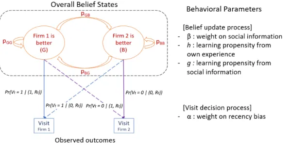
Therefore, the consumer’s overall belief update depends on the three behavioral pa-rameters: β captures weight on social information over own information, h captures responsiveness to her own experience, andgcaptures responsiveness to social informa-tion. For example, consider a consumer with prior beliefGat the beginning of periodt
who chooses to visit firm 2 and is satisfied. If she disregards social information (β= 0), then with probability hshe switches her belief to Bafter that period. However, if this consumer gets more positive social information about firm 1 (i.e., better reputation than firm 2) and disregards her own experience (β = 1), then she sticks to her prior belief that firm 1 is better (G) with probability one. More likely is the case that the consumer gives weight to both her own experience and social information (0 < β < 1). Then the transition probability in our model becomesP=β·
1 0 g 1−g +(1−β)· 1−h h 0 1 . 2.1.2. Visit Decision
To define the visit probability, letRt = Y1t−2Y2t+1 ∈ {0,0.5,1}combine the recency
vari-ables Y1t and Y2t to represent ‘which firm is better’ from the most recent service
en-counter. Previous research in sequential learning shows that human decision makers are prone to recency bias, and respond to both their most recent experience and overall past experience [30, 43, 51]. Evidence also indicates that the past outcomes, except the most recent outcome, have a similar impact on future choices [28, 54]. Although exponen-tial smoothing gives a higher weight to more recent experiences, it differs from recency bias. Therefore, we allow a consumer to associate a higher weight with her most recent experiences given her overall belief. Thus, we model the probability of visiting firm 1 in time periodtgiven current state (At,Y1t,Y2t) as:
Pr(Vt = 1|(At,Y1t,Y2t))= (1−α)·At +α·Rt, (1.5)
where α ∈ [0,1] measures the extent of recency bias. Ifα = 0, the consumer’s visit decision is driven purely by her overall belief (that is updated through own and social learning), if α = 1, the choice is purely myopic, and if 0 < α < 1, the consumer is influenced by her overall belief, yet exhibits recency bias at the same time.
Figure 1.1 shows the transition diagram between the belief states, the outcome (visit) probability, and the related behavioral parameters in this process.
If we alternatively, expand this to our eight-state Markov Chain, the consumer’s decision process and learning can be captured as in figure 1.2 shows our that captures the consumer’s decision process and learning.
Now, we show the complete transition matrix and store visit probabilities in this Markov chain. Expanding the consumer’s visiting probability of firm 1 conditional on the statex,v1
x is defined as following.
v11= Pr(visit firm 1 |(G,1,1))=(1−α)·1+α· 12 =1−0.5α
Figure 1.1: Transition diagram: transitions between the hidden belief states and the visit probability
v13= Pr(visit firm 1 |(G,0,1))=(1−α)·1+α· 01 =1−α v14= Pr(visit firm 1 |(G,0,0))=(1−α)·1+α· 12 =1−0.5α v15= Pr(visit firm 1 |(B,1,1))=(1−α)·0+α·12 =0.5α v16= Pr(visit firm 1 |(B,1,0))=(1−α)·0+α·11 =α v17= Pr(visit firm 1 |(B,0,1))=(1−α)·0+α·01 =0 v18= Pr(visit firm 1 |(B,0,0))=(1−α)·0+α·12 =0.5α
Again, a consumer’s visit probability of firm 2 given the state x, v2x, is 1− v1x. This
structure in current configuration imposes a consumer’s higher likelihood of revisiting the firm with satisfactory experience. For example,v13 = 1−αrenders that a consumer is not likely to choose firm 1 with certainty even if her prior belief is G, but with positive probability 1−α. The probability of visiting firm 1 decreases with the weight on the most recent experience, however, this decrease in probability is smaller inv1
1, if her most
recent experience from the firm 1 was also satisfactory.
It is notable that own learning propensity is embedded with probability h. For instance, if the consumer was dissatisfied from firm 1 while the belief being G, she switches her overall belief to B with probability h. This gives us 8 × 8 transition matrix Pby combining the store visit probabilities and the switching propensity. Let
P = [[PGG,PGB],[PBG,PBB]], where PGB defines the transition sub-matrix from states
G to B and PGG,PBG, and PBB have analogous definitions. The values of the transition
probabilities are: PGG = v11q1+v21q2(1−h) v12(1−q2) v11(1−q1)(1−h) 0 v2 2q2(1−h) v12q1+v22(1−q2) 0 v12(1−q1)(1−h) v1 3q1 0 v13(1−q1)(1−h)+v23q2(1−h) v23(1−q2) 0 v1 4q1 v 2 4q2(1−h) v 1 4(1−q1)(1−h)+v 2 4(1−q2)
PGB= v21q2h 0 v11(1−q1)h 0 v22q2h 0 0 v12(1−q1)h 0 0 v13(1−q1)h+v23q2h 0 0 0 v24q2h v14(1−q1)h PBG= v15q1h v25(1−q2)h 0 0 0 v16q1h+v26(1−q2)h 0 0 v17q1h 0 0 v27(1−q2)h 0 v18q1h 0 v28(1−q2)h PBB= v15q1(1−h)+v25q2 v52(1−q2)(1−h) v15(1−q1) 0 v26q2 v16q1(1−h)+v62(1−q2)(1−h) 0 v16(1−q1) v17q1(1−h) 0 v17(1−q1)+v27q2 v72(1−q2)(1−h) 0 v1 8q1(1−h) v28q2 v18(1−q1)+v28(1−q2)(1−h)
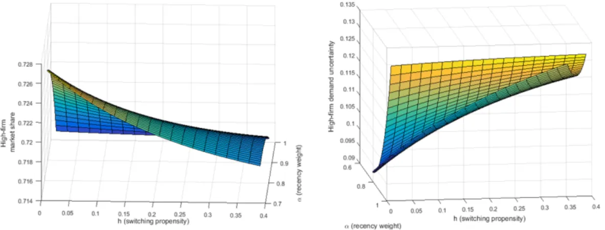
This completes the description of the eight-state Markov chain model of consumer behavior in response to previous service experiences. Using the stationary distribution of this model, we can conduct preliminary simulation to generate the steady-state market share and the variance of the High-firm. Figure 1.3 and 1.4 show the impact of theαand
hon predicted demand. Figure 1.3 shows that the long-term market share of High-firm decreases and the variance increases with more weight on recency bias (α). Figure 1.4 shows that the long-term market share of High-firm decreases and the variance increases with higher learning propensity (h).2
For instance, consider the transition probability from (G,1,0) to (B,1,1), which has a value ofPr(Visit Firm 2 |state = (G,1,0))·q2·h. In order for this transition to occur,
2These simulation results display non-monotonicity due to the non-linearity of our model. Thus, we report only the reasonable range of parameters in the Figure 1.3 and 1.4.
Figure 1.3: Preliminary simulation result: Expected market share and the variance of High-firm with respect to the weight on recency biasα
Figure 1.4: Preliminary simulation result: Expected market share and the variance of High-firm with respect to the own learning propensityh
the consumer must choose to visit firm 2 and experience satisfaction. This probability is Pr(visit the firm 2 | state = (G,1,0))·q2. Further, the consumer, who previously
believed that firm 1 had better quality, changes her belief from G to B with probability
h. Combining these steps of the decision process gives us the transition probability. This characterizes the consumer’s decision process affected by a two-fold memory structure with (1) an (unobserved) overall belief formed by past experiences up to timet, and (2)
the most recent experience (observed) from a consumer’s visit to each firm.
2.1.3. Social Information
To model social information (SI, hereafter), we partition the N consumers into disjoint subsets that represent social networks. We retrieve two different types of social informa-tion from the network and provide them to consumers separately at the end of periodt. The first type, ‘share-based’ SI, is defined as the percentage of consumers in a network who visit each firm. This information gives an estimate of market share of each firm in the network, or equivalently, the average of visit probabilities of consumers in the network, in periodt. We say that share-based SI favors firm 1 (firm 2) if the observed market share of firm 1 (firm 2) is higher than that of firm 2 (firm 1), and is ambiguous if market shares are identical.3 The second type, ‘quality-based’ SI, is defined as the percentage of consumers in a network who had satisfactory outcomes at the two firms. This information provides estimates ofq1andq2from the experiences of consumers in
the network in periodt. Quality-based SI is undefined if no consumer in the network visited a firm in periodt. Similar to share-based SI, we say that quality-based SI favors firm 1 (firm 2) if the observed average satisfaction from firm 1 (firm 2) is higher than that from firm 2 (firm 1), and is ambiguous if satisfaction rates are identical.4 Thus, we incorporate these two different types of social information in the belief formation for each consumer.
Social information introduces a complexity that the transition matrix of a consumer is a function of the states and transitions ofallconsumers in her network. Thus, the states and transitions of consumers are correlated with each other. We simulate this correlation in our experiment by generating social information dynamically in each period using the
3We say that 50% visited firm 1 and 50% visited firm 2.
4We report the satisfactions from each firm as it is, so it does not matter when they are identical. If no consumers choose one firm, we just say no one visited that firm.
actual choices and visit outcomes of consumers. Thus, the experiment moves lock step from one time period to the next.
This completes the description of our model. It is a parsimonious model with only four parameters to be estimated. We considered alternative formulations of learning from historical experiences, but the state space of the model explodes quickly. Even a regression-based robustness test of our model (presented in Section 1.5.1) requires more parameters than the Markov chain model. The simplified binary states of belief of our model reflect the real-world where consumers often remember only the superior-ity/inferiority of a firm relative to its competitors rather than keeping track of each firm’s quality level in absolute scales. By keeping the dimension of the state space minimal, our model is parsimonious, yet it predicts demand, and captures the salient aspects of a consumer’s probability of visiting a store, namely, the overall beliefs about quality and the recency bias. Moreover, in forming the overall belief, two learning components from the consumer’s own experience and social information are integrated into the latent state variable.
1.2.2
Hypotheses
Our first hypothesis tests the validity of the model. We hypothesize that consumers are susceptible to recency bias, but also form beliefs using own and social information, and utilize these beliefs in their store visit choice.
Hypothesis 1
(i) Consumers demonstrate moderate levels of recency bias (α > 0), and own-learning propensity (h>0).
social-learning propensity (g> 0).
Based on this hypothesized behavior of consumers, we can characterize demand by computing the following metrics from the estimated model: (1) the market share of each firm, (2) the variance of its demand, and (3) the speed of convergence of demand distribution to the steady state. We hypothesize that the availability of social information improves these metrics for the higher quality firm, i.e., firm 1.
Hypothesis 2
Comparing the marketplace under social information with the marketplace without so-cial information, the High-firm
(i) realizes a higher market share,
(ii) realizes a lower variance of demand, and
(iii) has a faster rate of convergence of its market share to the steady state value.
To set up this hypothesis, we reason as follows. When consumers are not exposed to SI, their learning is from own experiences alone. However, a consumer visits only one firm in each period, and thus, can update beliefs about one firm in each period. When they are exposed to SI, human subjects will utilize the increased availability of information (β > 0). Further, both types of social information are correlated with the true quality of the firms. Thus, consumers exposed to SI will learn at a faster rate that firm 1 is the higher quality firm. Moreover, their choices will be correlated with each other, which would lead to a higher market share for firm 1 and a lower variance of demand. Finally, when a consumer is exposed to SI, it may increase the relative weight on beliefs and decrease the extent of recency bias α. This factor would also result in higher market share and lower variance of demand for firm 1.
benchmarking our experimental results against outcomes from two models in the lit-erature: the Wins-Stay-Lose-Shift (WSLS) model [63] and Bayesian learning [9, 31]. WSLS consumers, at one extreme, are fully myopic and respond to the most recent ex-perience only. Bayesian learners, at the other extreme, utilize all previous exex-periences. Both these models are based on own experiences; they do not incorporate social infor-mation.
1.2.3
Parameter Estimation
We estimate the parameters of our model using maximum likelihood estimation (MLE). Our data set consists of the observed visit decisions, satisfaction outcomes, and social information for all consumers for all t. Thus, we compute the likelihood of observed visit decisions as a function of the model parameters and maximize it using the data set.
Letπitbe a vector denoting a probability distribution defined over the state spaceSof
the Markov chain for consumeriin periodt. We callπitas the belief-state probabilities.
To initialize the model, we assume that each consumer has an equal probability of being in any of the eight states att =1, and moreover, she has an equal probability of visiting either firm. Subsequently, the visit decisions and outcomes allow us to defineI{Go},I{Bo},
I{Gs}, and I{Bs} for all consumers in all periods. Using these values and the transition
matrix defined in (1.4), the new belief-state probabilities can be computed iteratively in period t+ 1 from πit. The next step is the setting up of the likelihood function. The
likelihood of consumer i visiting firm 1 in period t is given by P
Sit∈Sπit(Sit)Pr(Vit =
1 | Sit). Likewise for the likelihood of visiting firm 2. Thus, the likelihood is also
calculated iteratively as a function of the evolving belief-state probabilities, historical outcomes, and historical social information up to periodt−1. Next, we determine the
parameters that jointly maximize the loglikelihood of observed visit choices. ˆ α,β,ˆ h,ˆ gˆ = arg max α,β,h,g X i,t
logL(α, β,h,g;Vit,Y1it,Y2itfor alli,t)
= arg max α,β,h,g
X
i,t
logPr(Vit|α, β,h,g).
We estimated the parameters using both a constrained non-linear optimization method and grid search. Both methods yielded consistent results. The estimated parameters are discussed in Section 1.4.1.
After parameter estimation, we calculate the long-term market share, variance of de-mand, and rate of convergence towards steady state for each firm. Withα, β,h,g > 0, we have an irreducible, aperiodic, and regular Markov Chain on the finite state space. Therefore, there exists a stationary distributionπ =limt→∞πit. This stationary
probabil-ity of the hidden belief states and the visit probabilities (1.5) allow us to calculate the long-run market share and variance of demand for firm 1. Additionally, the convergence speed of πit toπ is determined by the size of the second-largest eigenvalue, λ2, of the
transition matrix. This metric shows how quickly a consumer’s belief-state probability converges to its stationary distribution. It thus indicates how fast a firm benefits from social information compared to the scenario without social information. We compute the convergence speeds under different treatments in our model in Section 1.4.4 and we explain in Appendix 1.7.2 why the second-largest eigenvalue (SLE) determines the convergence speed.
1.3
Experimental Design
We design our experiment to replicate the setting defined in Section 1.2. Each subject plays the role of a consumer choosing among two stores competing through their service
quality. In each round, after a subject chooses to visit a store, the computer returns either Satisfaction or Dissatisfaction from the chosen store, generated by a Bernoulli distribution, where the mean service quality levels of each firm,q1andq2, are unknown
to the consumer.
The experiment follows a between-subject design. Each subject participates in one treatment among 2×3 possible combinations given by two different quality competition settings and three information settings. For the quality competition settings, we use two different sets of mean service levels (q1,q2)= (0.8,0.5), which we refer to as alarge-gap
competition condition and (q1,q2) = (0.55,0.5), referred to as asmall-gapcompetition
condition. To investigate the effect of different types of SI, we use three information settings: (1) a control treatment with no SI (2) a share-based information treatment, and (3) a quality-based information treatment. In the share-based treatment, in each period, we provide subjects with the percentage of visitors to each firm as additional feedback, e.g., “For this period, 30% of your acquaintances visited store A, and 70% of your acquaintances visited store B.” In the quality-based treatment, in each period, we display the satisfaction rate of consumers for each firm, e.g., “For this period, 60% of your acquaintances who visited store A experienced satisfaction, and 20% of your acquaintances who visited store B experienced satisfaction.” Thus, we distinguish be-tween two different kinds of social information that are typically available to consumers in practice.
As mentioned previously, in the SI treatments, we interactively collect the decisions made by the subjects in each period to provide information in the following period, instead of using pre-generated outcomes. Using real-time information of the actual sub-jects’ choices/experiences better captures the true process of SI generation in practice. Moreover, we randomize the social network in each period. Specifically, each session of
the experiment consists of 18 subjects, who are randomly placed into a group of nine in each period. In the treatments with SI, after each round, all of the decisions are collected from the eight other people in a subject’s group and used as the SI for that subject. Thus, after each period of decision making, each subject is presented with not only her own service encounter but also certain social information regarding eight other subjects. We inform subjects that all feedback provided, including the information on others’ visits and experiences, is generated from their actual choices and real-time experiences in the laboratory.
There are 36 subjects in each of the six treatments. A subject’s main task is to choose either store A or B on the computer screen in each time period. This decision task is conducted for 40 periods. The arrangement of displaying high- and low- quality store as store A or B on screen is randomized across subjects (which is unknown to them). For the duration of the experiment, subjects can observe their history of choices, outcomes, and SI, when applicable. After completing 40 periods of decision making, we ask the subjects to provide their own estimate of service quality of each firm. To maintain incentive compatibility for this post-experiment question, we award subjects additional earnings if their answer lies within a certain range of the true average service quality.
Subjects in our experiment were recruited from a university located in the northeast U.S. The average total compensation was approximately $20 per participant. Each time a subject receivedsatisfactionfrom her visit choice, one point was given, corresponding to $0.50. These earnings were totaled across the 40 rounds and added to a $5 partic-ipation fee. Each session lasted about 40 minutes, and the software was programmed using the z-Tree system [29]. Instructions, screen shots, and more details about our experimental design are available upon request.
1.4
Results
In this section we first report the parameters of our Markov chain model, estimated us-ing the experimental data, in subsection 1.4.1, and conclude on Hypothesis 1. Then, we summarize our three demand characteristics of interest (market share, demand uncer-tainty, and convergence speed), in subsections 1.4.2, 1.4.3, and 1.4.4, and conclude on each component of Hypothesis 2.
1.4.1
Parameter Estimation
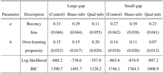
In Table 1.1, we first report the two-parameter model estimation results, without consid-eration of SI (i.e. h = g = 0). The behavioral parameters, all significant, demonstrate that consumers show moderate levels of recency bias and learning propensity under all treatments. Moreover, the presence of SI appears to create a difference in the amount of recency bias. For instance, for both levels of service competition, large-gap and small gap, α is lower under quality-based SI, indicating that consumers are less susceptible to a recency bias when quality-based SI is provided. Also, note that, when interpreting the magnitude of the estimates, only comparisons across different types of SI within a particular level of service competition are meaningful (since different values ofq1 and
q2are used in different service competition treatments).
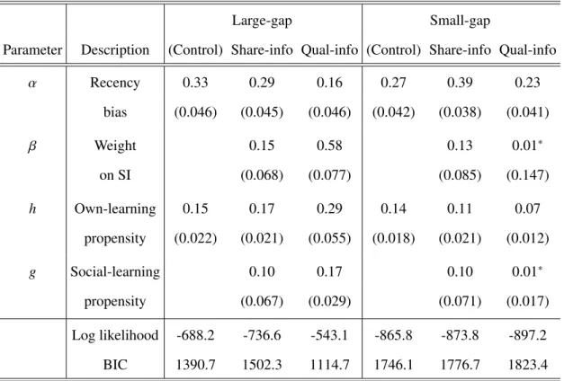
In Table 1.2, we report the estimate results using all four parameters. Note that the most striking effect of social learning exists under quality-based SI under large-gap competition. Under this treatment, consumers utilize quality-based SI significantly (β = 0.58), and display relatively low recency bias (α= 0.16). We also observe higher own-learning (h = 0.29) and social-learning (g = 0.17) propensities than the other
Table 1.1: Two parameter model estimates
Large-gap Small-gap
Parameter Description (Control) Share-info Qual-info (Control) Share-info Qual-info
α Recency 0.33 0.29 0.11 0.27 0.39 0.23 bias (0.046) (0.044) (0.055) (0.042) (0.038) (0.041) h Own-learning 0.15 0.15 0.20 0.14 0.11 0.07 propensity (0.022) (0.017) (0.020) (0.018) (0.020) (0.012) Log likelihood -688.2 -738.6 -557.0 -865.8 -874.9 -897.2 BIC 1390.7 1491.7 1128.2 1746.1 1764.3 1808.9
Note: All parameters are significant withp<0.01. Standard errors from inverse Hessian matrix are in parentheses.
treatments, which means a consumer’s overall belief transition is actively influenced by both learning from their own recent experience and via the social information about others’ experiences.
In all four SI treatments, in Table 1.2, we continue to observe that consumers’ belief switching is more influenced by their own experience than others (h > g). In addi-tion, SI is utilized by consumers under share-based SI treatments (β > 0), despite the fact that this information does not directly signal the true service quality of the firms. However, when we compare the overall fit in Table 1.2 to that in Table 1.1, it would appear as though including the two SI-related parameters,βandg, only improves the fit in quality-based SI under large-gap competition, which is evidenced by the smaller BIC value. Furthermore, a series of Likelihood Ratio tests confirms that the four parameter model, which explicitly incorporates the impact of SI, is preferred in the quality-based SI treatment with large-gap competition (p<0.001).
Table 1.2: Four parameter model estimates
Large-gap Small-gap
Parameter Description (Control) Share-info Qual-info (Control) Share-info Qual-info
α Recency 0.33 0.29 0.16 0.27 0.39 0.23 bias (0.046) (0.045) (0.046) (0.042) (0.038) (0.041) β Weight 0.15 0.58 0.13 0.01∗ on SI (0.068) (0.077) (0.085) (0.147) h Own-learning 0.15 0.17 0.29 0.14 0.11 0.07 propensity (0.022) (0.021) (0.055) (0.018) (0.021) (0.012) g Social-learning 0.10 0.17 0.10 0.01∗ propensity (0.067) (0.029) (0.071) (0.017) Log likelihood -688.2 -736.6 -543.1 -865.8 -873.8 -897.2 BIC 1390.7 1502.3 1114.7 1746.1 1776.7 1823.4
Note:∗Parameters are not statistically significant. Standard errors from inverse Hessian matrix are in
parentheses.
the model at an individual level. Unsurprisingly, there is some heterogeneity in the estimates among subjects, but the average values of the parameters do not deviate sig-nificantly from the aggregate-level estimates presented above. Therefore, to summarize, Hypothesis 1 -(i)is fully supported - subjects demonstrate moderate levels of recency bias and own-learning propensity, whereas Hypothesis 1 -(ii) is partially supported -consumers directly respond to quality-based SI when there is a large-gap in the level of service competition.
Prediction Accuracy of the Model
One important way in which firms can benefit from understanding the SI-induced change in consumer behavior is by improving their demand forecasting. Here, we report the predictive performance of our model by simulating the choice paths of consumers. Using the estimated parameters from Table 1.2, we generate the simulated choice paths of consumers, and thus, predict the market share.
Table 1.3: Prediction error in the hold-out samples (period 31-40)
Large-gap Small-gap
(Control) Share-info Qual-info (Control) Share-info Qual-info
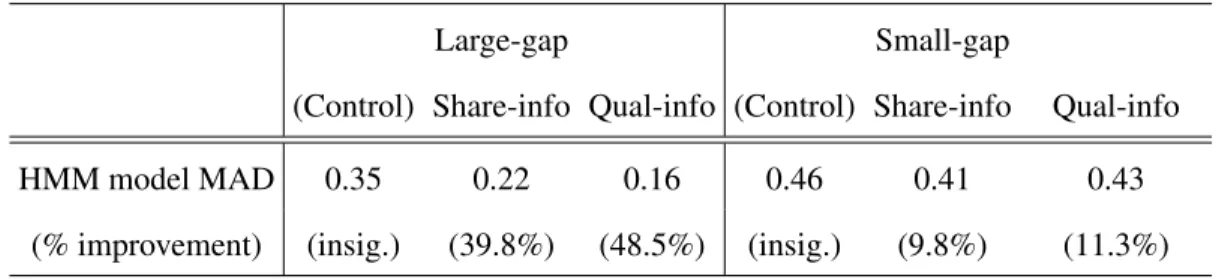
HMM model MAD 0.35 0.22 0.16 0.46 0.41 0.43
(% improvement) (insig.) (39.8%) (48.5%) (insig.) (9.8%) (11.3%)
Note: “% improvement” compared to the WSLS prediction (no improvement under control group).
In Table 1.3, we present the mean-absolute deviations (MAD) of the model’s (HMM) prediction to the observations in periods 31-40. It also illustrates the percent improve-ment from the model’s predictions compared to that of the WSLS consumers’ simulated choice paths. One can immediately observe that the prediction errors are smaller under SI treatments, and that, with SI, the model better explains the choice behavior of con-sumers compared to the WSLS prediction. Particularly, the prediction accuracy of the model increases considerably with the presence of SI under large-gap competition.
1.4.2
Market Share
To understand the consequences of this behavior on the firms, we next turn to firm-level demand characteristics. Our first firm-level demand characteristic of interest is average
market share. Given that the proportion of consumers choosing the High-firm and Low-firm sums up to one, for presentation purposes, we report only the High-Low-firm’s market share. In Table 1.4, we provide the average market share of the High-firm in each treat-ment, along with two benchmarks: the predicted market share if consumers followed a Win-Stay-Lose-Shift (WSLS) strategy (α = 1), or behaved like perfect Bayesian con-sumers (α = 0).5 As seen in Table 1.4, under both competition levels, the market share of the High-firm in the control treatment falls between the predicted market share of WSLS and Bayesian consumers – human subjects chose the High-firm more frequently than WSLS consumers, but not as often as Bayesian consumers. Turning to the SI treatments, it is interesting to note that the average market share of the High-firm in the quality-based information treatment under large-gap competition (85.6%), is nearly identical to the Bayesian prediction (86.6%), whereas under small-gap competition, it is almost the same (52.1%) as the WSLS prediction (52.5%).
To conclude on Hypothesis 2 -(i), we must compare the average market share of the High-firm under different types of SI (Table 1.4). Beginning with the share-based infor-mation treatments, one can see that the average market share of the High-firm is virtually identical to the control treatment, for both levels of competition. However, the average market share under quality-based information is significantly different compared to the control treatment, albeit in opposite directions, depending on the level of competition. In particular, under large-gap competition, the average market share with quality-based information is 85.6%, which is significantly higher than both the control and share-based SI conditions (t-tests, both p < 0.01). On the other hand, under small-gap competition, the market share of the High-firm under quality-based information is actually lower than the control treatment, weakly significantly so (t-test,p<0.10). Note that this final result implies that the Low-firm, under small-gap competition may benefit from quality-based
Table 1.4: Market share of the High-firm under different SI treatments
SI treatment Large-gap Small-gap
(Control) 70.0% 56.7% (1.2%) (1.0%) Share-based info 70.8% 58.1% (2.0%) (1.3%) Quality-based info 85.6%∗∗∗ 52.1%∗∗ (1.4%) (1.3%) Bayesian benchmark 86.6% 62.9% (2.0%) (0.8%) WSLS benchmark 67.6% 52.5% (1.8%) (1.7%)
Note:∗∗p<0.01,∗p<0.1 t-tests comparing SI treatments to Control. Standard errors over time in
parentheses.
information, as a reduction in the High-firm’s market share increases the market share of the Low-firm, from 43.4% (High-firm 56.7%) to 47.9% (High-firm 52.1%). Therefore, Hypothesis 2 -(i)is partially supported, for quality-based information under large-gap competition.
The contrasting market share results under large and small-gap competition in the quality-based information treatment warrants additional discussion, and can be under-stood by returning to the behavioral parameter estimates in Table 1.2. Specifically, re-call that consumers’ actively use quality-based SI under large-gap competition, but not small-gap competition. This implies that a firm’s promotion of quality-based informa-tion can magnify the impact of the actual quality gap between the competitors with respect to their market share. Thus, quality-based information can overly detriment the
Low-firm under large-gap competition, but provide potential benefits under small-gap competition, relative to the firm’s true quality difference with its competitor.
Consumer Satisfaction
Increased market share is clearly desired by firms, but with it comes an additional benefit when there is SI. That is, a higher market share allows a firm a better chance of providing a satisfactory experience for consumers, which not only impacts a consumer’s willing-ness to revisit the same firm, but also re-generates positive social influence for others. Indeed, when positive information is naturally generated through satisfactory outcomes, as in our setting, the market share can further favor one of the competing firms.
Table 1.5: Average satisfaction rates of all subjects in each treatment, and the sub-jects visiting each firms
Large-gap Small-gap
Description (Control) Share-info Qual-info (Control) Share-info Qual-info
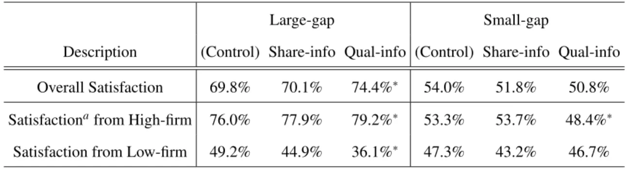
Overall Satisfaction 69.8% 70.1% 74.4%∗ 54.0% 51.8% 50.8%
Satisfactionafrom High-firm 76.0% 77.9% 79.2%∗ 53.3% 53.7% 48.4%∗
Satisfaction from Low-firm 49.2% 44.9% 36.1%∗ 47.3% 43.2% 46.7%
Note:∗p<0.01, significant difference with the subjects in other SI treatments.
Table 1.5 depicts the overall satisfaction rates of consumers who visit each firm, by treatment. One interesting observation is that the satisfaction rates for each firm, which theoretically should be the same across different SI treatments, within the same level of quality competition, show systematic differences. Consider the second and third rows of numbers, which report the average satisfaction rate of from subjects from each firm. One might note that all of these numbers are below the firms’ true average service qualities, and, in certain SI conditions, the Low-firm achieves an exceptionally low
sat-isfaction rate. This is because consumers do not switch randomly between firms, rather, they may be more inclined to switch after a failed service (and depending on the SI). For example, in the quality-based information treatment in large-gap competition, the consumer satisfaction rate from the Low-firm is only 36.1%, and this is considerably lower than the consumer satisfaction under the control treatment in large-gap competi-tion, 49.2%. Instead, the average satisfaction rate should be close to 50%. However, in general, when a consumer visits the Low-firm, there is a relatively higher likelihood of receiving a dissatisfactory experience. Combined with quality-based SI, the consumer may also receive positive information about the High-firm, causing the consumer to switch to the High-firm. Once at the High-firm, however, there is a lower likelihood of a dissatisfactory experience, and to see SI that would cause them to switch back to the Low-firm. The net result is that the High-firm can achieve an even greater advantage in terms of providing satisfactory experiences to consumers, under quality SI in large-gap competition.
This result is consistent with Park et al. [60], as a low estimate of service quality leads to longer time between a consumer’s subsequent visits, and so, less occasion to learn the service quality offered by a firm. We conclude that under the circumstances where consumers are not well informed about the true service level offered by firms, their dependence on SI affects the chances for firms to provide satisfaction to consumers, thus affecting the market share and profitability altogether.
1.4.3
Demand Uncertainty
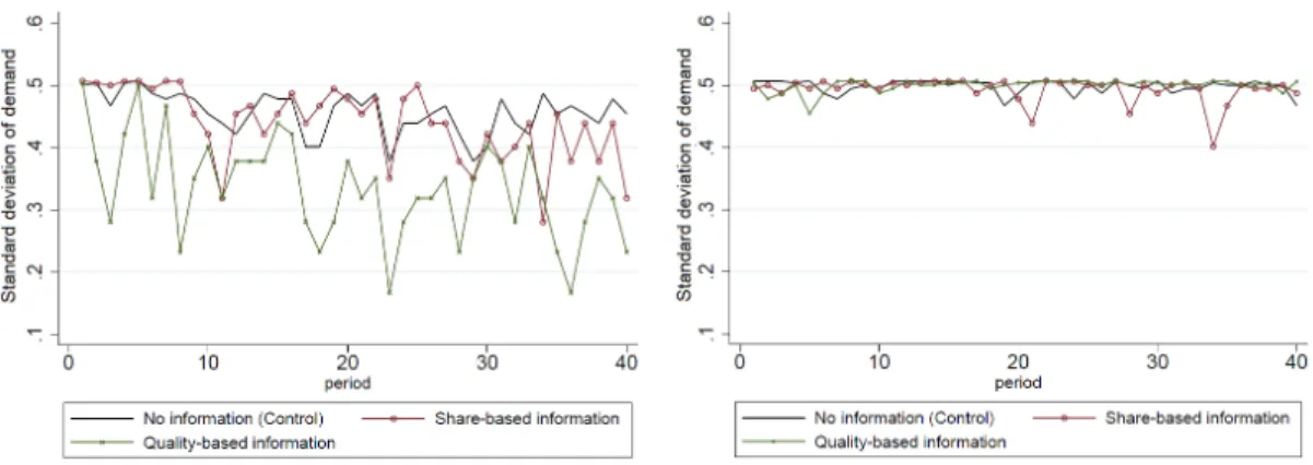
Our second firm level characteristic of interest pertains to the uncertainty of demand. Figure 1.5 plots the standard deviation of demand (market share) over time. One can see
Figure 1.5: Demand uncertainty under different types of SI (standard deviation) under Large-gap (left) and Small-gap (right) treatment
that demand uncertainty varies across SI treatments. In particular, under quality-based information, for all decision periods, we observe a significant reduction in demand un-certainty in large-gap competition (t-tests, across all p < 0.01). Combining this with our previous findings on average market share implies that, when the firm with sig-nificantly higher quality promotes quality-based information, it not only benefits from increased market share, but from reduced demand uncertainty as well. In such a case, the Low-firm will lose a significant portion of its consumers to its competitor, achieve considerably lower market share, and also face higher demand uncertainty. Therefore, like the impact of SI on market share, Hypothesis 2 -(ii), which states that the vari-ance of demand will be reduced with social information, is partially supported, under quality-based information with large-gap competition.
Switching Behavior
To further investigate demand uncertainty, we also looked into the individual consumers’ choice behavior (since the variance of demand only captures the number of visitors rather than the composite of consumers). To this end, the left-hand side of Table 1.6 shows how frequently an average consumer switches between firms, and the right-hand
side of Table 1.6 shows the average time each subject spends in one firm before switch-ing, along with the predictions according to the Bayesian and WSLS benchmarks (the right hand side can be interpreted as the averageSojourn timebetween transitions among the states out of 40 total periods).
Table 1.6: Percentage of time switching and expected sojourn time over 40 peri-ods
% of time switching Ei(S o journ time)
Large-gap Small-gap Large-gap Small-gap
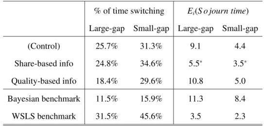
(Control) 25.7% 31.3% 9.1 4.4
Share-based info 24.8% 34.6% 5.5∗ 3.5∗
Quality-based info 18.4% 29.6% 10.8 5.0
Bayesian benchmark 11.5% 15.9% 11.3 8.4
WSLS benchmark 31.5% 45.6% 3.5 2.3
Note:∗p<0.01 for t-tests with the control treatment.
Compared to the theoretical benchmarks, in Table 1.6, it appears that subjects stay in one firm longer than the WSLS consumers, but shorter than the Bayesian consumers, on average across all treatments. Comparing treatments to one another, under share-based information, average sojourn time is significantly lower than the other treatments, both in large-gap and small-gap competition. Furthermore, while not depicted, we find that all of the subjects in the share-based information treatment switched at least once, whereas some subjects never switched at all in the other treatments.
Taking this analysis a step further, we label the subjects who stay in one firm more than 10 consecutive periods on average, i.e., individuals withE(S o journ time)>10, as ‘Loyal consumers,’ and subjects who switch frequently, i.e., withE(S o journ time)< 2, as ‘Frequent switchers.’ We present the percentage of these subjects in each treatment in
Figure 1.6: Percentage of frequent switchers and loyal consumers under different SI treatments 13.9% 8.3% 0.0% 19.4% 22.2% 16.7% 22.2% 11.1% 36.1% 8.3% 0.0% 5.6% 0% 5% 10% 15% 20% 25% 30% 35% 40%
Control Share-based info Quality-based info Control Share-based info Quality-based info
Large-gap Small-gap
Frequent switchers, Ei(sojourn)<2 Loyal consumers, Ei(sojourn)>10
Frequent switchers, Ei(sojourn)<2
Loyal consumers, Ei(sojourn)>10
Figure 1.6. As one can see, in the quality-based information treatment under large-gap competition, more than 35% of subjects behave like loyal customers, on average. On the other hand, in the share-based information treatment, the proportion of loyal customers is the lowest, for both levels of competition (11% under large-gap, 0% under small-gap). This evidence suggests that quality-based information boosts loyalty for the High-firm under large-gap competition, whereas share-based information reduces loyal customers and promotes switching regardless of the level of competition.6
6To test whether the deviation from Bayesian choice can be explained by subjects’ most recent expe-rience and by SI, we use a Logit model withP(Deviation f rom Bayes Choice =1|Xi) as a dependent
variable, which captures only (unnecessary) switching of subjects to a firm with lower estimate of service quality each period. We observed that the exploration to the Low-firm decreases with the most recent satisfaction from the High-firm, and increases with the recent satisfaction from the Low-firm. More in-terestingly, both of the SI types significantly affected the result: share-based information increases this exploration to the firm with the lower estimate of service quality, whereas positive quality-based informa-tion from the High-firm decreases unnecessary switching. This evidence confirms that overall deviainforma-tions from the Bayesian choices increase under share-based information, whereas the valence of quality-based information directly impacts the switching of the consumers.
1.4.4
Convergence Speed
We now consider our third demand characteristic, by analyzing the convergence speed of the transition probability (between the unobserved belief states of our model).
Table 1.7 reports the convergence measures based on our current model assumption where the demand is formed by unobserved belief states (G or B). In the long run, how the overall belief states of aggregate consumers settles to its equilibrium determines the market share convergence speed.
Table 1.7: Stationary probability (π) of the belief transition matrixPand the con-vergence speed measures
Competition treatment SI treatment
Stationary dist. Minimum periods SLE
π=[πG, πB] forP ∈ {π±0.01} λ2
(Control) [ 0.666 , 0.334 ] 26 periods 0.847
Large-gap Share-based info [ 0.717∗, 0.283 ] 25 periods 0.843
Quality-based info [ 0.791∗, 0.209 ] 18 periods 0.782
(Control) [ 0.531 , 0.469 ] 28 periods 0.864
Small-gap Share-based info [ 0.562 , 0.438 ] 35 periods 0.889
Quality-based info [ 0.512 , 0.488 ] 54 periods 0.929
Note:∗Limit probability of overall belief being G,π
G, is significantly higher thanE(Rt) observed from data.
SLE represents “second-largest eigenvalue.”
First, in Table 1.7 note that the stationary distribution of the overall belief being G, for large-gap competition, is highest in quality-based SI (πG =0.791), and in small-gap
competition, is highest in share-based SI (πG = 0.562). With the behavioral parameter
estimates in Table 1.2, and the different information set of each subject, we reconstructed the belief-transition probabilities Puniquely under different treatments, such that the limit probabilities and the convergence speed to equilibrium vary across treatments. A
higher stationary probability of the overall belief being G leads to a frequent visit to the High-firm. In short, the results here are consistent with our previous observations that the market share is highest in quality-based SI under large-gap competition, and high-est in share-based SI under small-gap competition (recall Table 1.4, which illustrated average market share by treatment).
Second, continuing in Table 1.7, consumers’ overall belief status converges to its stationary probability quickest in quality-based SI under large-gap competition. In par-ticular, within 18 periods, belief switching probabilities converge within the bound of 0.01 from the limit probabilities. The second-largest eigenvalue (SLE) is also smallest in this treatment (λ2 = 0.782), providing further support for fastest convergence to
sta-bility, making the demand forecast easier in earlier periods (please see Appendix 1.7.2 for a further discussion and technical details).
Third, in Table 1.7, note that the speed of the belief converging to equilibrium is significantly slower with SI treatments under small-gap competition. This is due to the average quality being similar between firms, under small-gap competition, and thus, the SI generated based on consumers’ experience naturally exhibits relatively higher variance. Therefore, this potentially leads to non-informative SI, and does not improve consumer learning and the settlement of beliefs.
In sum, our convergence analysis allows us to conclude that Hypothesis 2 -(iii) is supported under quality-based information in the large-gap competition treatment, but not across all SI treatments. Faster convergence speed is driven by the fact that, in our analyses on market share, the presence of quality-based information significantly favors the High-firm, which is compounded by a moderated recency bias and increased learning propensities, particularly under large-gap competition.