A bayesian approach to model-based clustering for panel probit models

(1)

econ

stor

www.econstor.eu

Der Open-Access-Publikationsserver der ZBW – Leibniz-Informationszentrum Wirtschaft

The Open Access Publication Server of the ZBW – Leibniz Information Centre for Economics

Nutzungsbedingungen:

Die ZBW räumt Ihnen als Nutzerin/Nutzer das unentgeltliche, räumlich unbeschränkte und zeitlich auf die Dauer des Schutzrechts beschränkte einfache Recht ein, das ausgewählte Werk im Rahmen der unter

→ http://www.econstor.eu/dspace/Nutzungsbedingungen nachzulesenden vollständigen Nutzungsbedingungen zu vervielfältigen, mit denen die Nutzerin/der Nutzer sich durch die erste Nutzung einverstanden erklärt.

Terms of use:

The ZBW grants you, the user, the non-exclusive right to use the selected work free of charge, territorially unrestricted and within the time limit of the term of the property rights according to the terms specified at

→ http://www.econstor.eu/dspace/Nutzungsbedingungen By the first use of the selected work the user agrees and declares to comply with these terms of use.

zbw

Leibniz-Informationszentrum Wirtschaft

Aßmann, Christian; Boysen-Hogrefe, Jens

Working Paper

A bayesian approach to model-based

clustering for panel probit models

Economics working paper / Christian-Albrechts-Universität Kiel, Department of Economics, No. 2009,03

Provided in cooperation with:

Christian-Albrechts-Universität Kiel (CAU)

Suggested citation: Aßmann, Christian; Boysen-Hogrefe, Jens (2009) : A bayesian approach to model-based clustering for panel probit models, Economics working paper / Christian-Albrechts-Universität Kiel, Department of Economics, No. 2009,03, http://hdl.handle.net/10419/27738

(2)

D

a bayesian approach to model-based

clustering for panel probit models

by Chrisitan Aßmann and Jens Boysen-Hogrefe

(3)

A Bayesian approach to Model-Based Clustering for

Panel Probit Models

Christian Aßmann∗

Institute of Statistics and Econometrics, Christian-Albrechts-Universit¨at Kiel, Germany

Jens Boysen-Hogrefe

Kiel Institute for the World Economy, Germany

April 15, 2009

Abstract

Consideration of latent heterogeneity is of special importance in non linear models for gauging correctly the effect of explaining variables on the dependent variable. This paper adopts the stratified model-based clustering approach for modeling latent heterogeneity for panel probit models. Within a Bayesian framework an estimation algorithm dealing with the inherent label switching problem is provided. Determination of the number of clusters is based on the marginal likelihood and out-of-sample criteria. The ability to decide on the correct number of clusters is assessed within a simulation study indicating high accuracy for both approaches. Different concepts of marginal effects incorporating latent heterogeneity at different degrees arise within the considered model setup and are directly at hand within Bayesian estimation via MCMC methodology. An empirical illustration of the developed methodology indicates that consideration of latent heterogeneity via latent clusters provides the preferred model specification compared to a pooled and a random coefficient specification.

JEL classification: C11; C23; C25

Keywords: Bayesian Estimation; MCMC Methods; Panel Probit Model; Mixture Modelling

∗_{Corresponding author. Tel.: +49-431-8803399; fax: +49-431-8807605.} E-mail address:

(4)

1 Introduction

The consideration of latent heterogeneity in panel models with relative short time horizons is of special importance in order to gauge correctly the influence of variables suggested by theory on the dependent variable. The often adapted strategy for linear models of pooling and computation of heteroscedastic or cluster robust variance estimates can not be applied to panel probit models for several reasons. In the presence of latent heterogeneity the pooled estimator is not guaranteed to be consistent, see Cameron and Trivedi (2005), and the computation of cluster robust variance estimates requires a sufficiently large number of observations per cross section. Furthermore, the natural approach of using fixed effects is often problematic since it causes the occurrence of an incidental parameter problem, see Lancaster (2000) for a general review and Greene (2004a) for a discussion focused on limited dependent variable models. Other common approaches to model latent heterogeneity are random coefficient specifications, which employ distributional assumptions on the heterogeneity and assume the orthogonality of latent heterogeneity and explaining variables, see Revelt and Train (1998), Mehndiratta (1996) and Ben-Akiva and Bolduc (1996) for applications.1 Alternatively, Fr¨uhwirth-Schnatter and Kaufmann (2008) suggest a stratified model-based clustering approach to deal with latent heterogeneity in the data generating process.2

Within this paper, the strategy to model latent heterogeneity via clustering, where the identifica-tion of clusters and affiliaidentifica-tion of panel members to clusters is simultaneously undergone to parameter estimation, is provided for panel probit models. Latent clusters for panel probit models have been considered by Greene (2004b) and Greene and Hensher (2003) in the context of maximum likelihood estimation. However, maximum likelihood estimation possibly fails to provide an accurate assess-ment of parameter uncertainty arising from genuine multimodality of the likelihood as discussed by Celeux (1998).

Hence, within this paper a Bayesian estimation approach is pursued, which is able to gauge pa-rameter uncertainty correctly in the presence of genuine multimodality via inspection of the posterior distribution. These advantages of the Bayesian approach are accompanied by the difficulty of label switching stemming from the invariance of the likelihood to relabeling of the clusters.3 As noted by Stephens (2000) dealing with label switching in Bayesian estimation is often done via incorporation of an identifiability constraint ensuring formal separation of the symmetric modes of the parameter space. Unfortunately, an identifiability restriction will possibly not suppress label switching

suffi-1_{Note that latent heterogeneity can also be addressed in non-parametric estimation environments, which are not}

subject of this paper.

2_{See Fraley and Raftery (2002) for a review of model based clustering in non-time series data.}

3_{In a maximum likelihood approach this problem is avoided as a single maximum (out of all symmetric ones) is}

(5)

ciently, since separation of the parameter space may only be weak causing poor parameter estimates. This paper employs a relabeling algorithm based on Stephens (2000) to deal with label switching, which is extended to deal with the considered model feature of stratified cluster probabilities.4

A further advantage of Bayesian estimation via MCMC methodology is the direct accessibility of a wide range of estimates of marginal effects incorporating latent heterogeneity at different de-grees. Since the MCMC methodology provides draws from the posterior distributions of parameters, estimates of marginal effects as moments thereof are easily calculated. In contrast to maximum like-lihood based estimation also the distributions of the marginal effects are directly accessible allowing to gauge the robustness of theoretical implications under latent heterogeneity.

Next to estimation conditionally on the number of clusters, the problem of determining the number of clusters is addressed within this paper. Several strategies to determine the number of cluster components are analyzed. Based on the MCMC output we use the marginal likelihood as a natural benchmark for assessing model fit. However, computation of the marginal likelihood asks for special efforts to ensure the accuracy of the involved numerical integration techniques. Therefore, we contribute an easy implementable alternative approach to assess model fit via a cross validation experiment.5 Thereby, our approach extends the range of available cluster strategies towards a Bayesian analysis of multivariate panel probit mixture models. We provide a simulation study highlighting the properties of these model selection devices.

Our results suggest via the conducted simulation study the ability of the marginal likelihood and the cross validation approach to select the correct number of clusters. In the empirical application using the data set of Bertschek and Lechner (1998) on firm innovation, we find that a model with 3 clusters is preferred and that it provides a better fit compared to a pooled or random coefficient specification. Implications for gauging theoretical issues are discussed in the context of marginal effects incorporation latent heterogeneity at different degrees.

This paper is hence organized as follows. Section 2 reviews the panel probit framework with random coefficients and stratified model based clustering. In Section 3 the Bayesian estimation methodology, the relabeling algorithm, the approach to calculate the marginal likelihood, and the considered cross validation design for determining the number of clusters are provided. The methods to identify the number of clusters are assessed within a simulation study in Section 4. An empirical

4_{See Handcock et al. (2007) for an application of the relabeling algorithm in the absence of meaningful identifiability}

constraints.

5_{Procedures for determining the number of clusters in finite mixture models are discussed in related contexts. Chen}

and Khalili (2008) discuss a penalized likelihood approach for univariate mixtures. Dunson et al. (2008) analyze a semi-parametric approach for univariate mixture models without stratified cluster probabilities. Ihswaran et al. (2001) employ approximate Bayes factors. Heard et al. (2006) contribute a hierarchical analysis for Bayesian curve fitting, while Ray and Lindsay (2008) analyze determination with a non-parametric quadratic risk approach.

(6)

illustration is given in Section 5, where the developed methodology is applied on the data set of Bertschek and Lechner (1998). Section 6 concludes.

2 Model Formulation

The setup of a pooled panel probit model is given as follows. Letyitdenote the observed dichotomous

variable, where i= 1, . . . , N, and t= 1, . . . , T. A link between observed explaining factors and the observed binary variables is provided via the latent variabley∗_it

yit =    1, ify_it∗ >0, 0, ify∗ it≤0, (1) where y∗_it=Xitβ+eit (2)

andeitis an independent identically normal distributed error term with unit variance. Pooling yields

the likelihood LP(Y|θ, X) = N Y i=1 T Y t=1 Φ [(2yit−1)Xitβ], (3)

where Φ(·) denotes the cumulative distribution function of a standard normal distribution.

An often considered approach to account for latent heterogeneity is to model random coefficients, see Train (2003). Henceβ is modeled as unit specific random variable

βiiid∼ N(b, W), (4)

whereW denotes the covariance matrix of the random coefficients andbdenotes the common mean vector for all individuals. This results in a likelihood function given as

LRC(Y|θ, X) = N Y i=1 Z Rp "_T Y t=1 Φ [(2yit−1)Xitβi] # f(βi|b, W)dβi, (5)

where p denotes the dimension of the vector of random coefficients. We will refer to this kind of modeling heterogeneity as a benchmark for modeling latent heterogeneity within the empirical illustration.

Alternatively, latent heterogeneity can be incorporated via latent clusters. Model-based clustering assumes a given number of cluster, where members of a cluster share the same parameters. Define

S = {Si}Ni=1, k = 1, . . . , K indicating the cluster membership for each individual. Conditional on

the cluster membership the latent model is given as

(7)

providing the joint density function f(Y|θ, X, S) = N Y i=1 T Y t=1 Φ [(2yit−1)XitβSi]. (7)

Fr¨uhwirth-Schnatter and Kaufmann (2008) propose two distinct ways in modeling the probabilis-tic structure of cluster membership. An a priori ignorant approach is to assume

Pr(Si =k|η1, . . . , ηK) =ηk, (8)

where ηk, k = 1, . . . , K −1 and ηK = 1−PKk=1−1ηk are the relative group sizes assumed to be

unknown parameters to be estimated. Alternatively, the probability of cluster membership may depend on certain unit specific factors, hence the probability is parameterized as a multinomial logit model given as Pr(Si=k|{γk}K_k₌₁−1, zi) = exp{ziγk} 1 +PK−1 k=1 exp{ziγk} . (9)

The individual specific variables zi stratifies hence the probability for a panel unit to belong to

cluster k.6 _{The logit structures coincides with the unconditional approach, when}_z

i includes only a

constant. Variables inzi may help to assign cluster membership. The model likelihood is given as

LC(Y|θ, X) = N Y i=1 K X k=1 "_T Y t=1 Φ ((2yit−1)Xitβk) Pr(Si=k|{γk}Kk=1−1, zi) # . (10)

Given these possibilities to consider latent heterogeneity within probit models different concepts for marginal effects arise. Conceptually, the marginal effect summarizing all parameters withinθ is given as

∂

∂xPr(y= 1|x=x, θ), (11)

where the function form of the derivative depends on the considered model structure for incorporation of latent heterogeneity. For the pooled model specification, the marginal effect is well known to be

M EP =φ(xβ)β, (12)

where φ(·) denotes the density of the standard normal distribution. For the model specification incorporating latent heterogeneity via random coefficients, the marginal effect takes the form

M ERC =

Z

φ(xβi)βif(βi|b, W)dβi, (13)

(8)

where the above given integral can be solved numerically or analytically, when assuming a normal distribution for the distributionf(βi|b, W).7 When latent heterogeneity is considered via modeling

of latent clusters, two concepts apply for assessment of marginal effects. First, a cluster specific measure is given as

M ECS =φ(xβk)βk, k= 1, . . . , K, (14)

while a cluster robust concept is8

M ECR= K

X

k=1

φ(xβk)βkPr(S=k|z,{γk}K_k₌₁−1). (15)

This set of different concepts are derived as measures for marginal effects and allow to gauge the influence of variables on the probability of an event under consideration of different forms of latent heterogeneity.9

3 Model Estimation

The inclusion of model structures capturing latent heterogeneity provides estimation problems, which are especially accessible to Bayesian estimation via MCMC methodology namely Gibbs sampling including Metropolis-Hastings updates. Using data augmentation, see Tanner and Wong (1987), the parameter vector is augmented to include the panel member specific cluster indices, which simplifies sampling from all other full conditional distributions.

Genuine estimation problems in the context of the model based clustering framework as a special type of mixture model are referred to in the literature as label switching and genuine multi modality, see Stephens (2000) and Fr¨uhwirth-Schnatter (2004). Label switching refers to the invariance of the likelihood under relabeling of clusters. The involved problem of label identification can be handled in different ways. The first solution is based on setting an identifying restriction on the parameter space, which hinders label switching. While the restrictions may be easily implemented it is important to find a restrictions, which efficiently separates the parameter space. If one chooses a restriction on parameters, which are almost identical within the clusters, the label switching problem is possibly still

7_{Note that the numerical solution is provided as a byproduct of the employed estimation routine, namely Gibbs}

sampling. However, the analytical solution is to be preferred for reasons of storing capacities and prevention of approximation errors.

8_{Alternatively to conditioning on a point} _z_{, the unconditional probability can be used (Pr(}_S ₌ _k_{) instead of}

Pr(S=k|z)).

9_{Note that also individual specific marginal effects might be interest, which can readily calculated based on individual}

(9)

present especially within the multivariate clustering considered here.10 Alternatively, as suggested by Stephens (2000), the output of the unconstrained Gibbs sampler can be post screened. These relabeling algorithms provide a decision theoretic tool to decide on the identification of clusters. While an identifiability constraint hindering label switching is not a priori known and hence chosen arbitrarily, the use of an relabeling device for post screening is computationally more demanding, but based on a decision theoretic criterion to deal with label switching.

Based on a finite sample argument, genuine multi modality is not accessibly to maximum like-lihood estimation and would hinder a correct assessment of parameter uncertainty. In contrast, posterior inference allows to display the occurrence of multimodality and hence provides a correct assessment of sample uncertainty in estimation yielding a further advantage of a Bayesian estimation approach.

The following sections provide the unconstrained sampler for the considered model framework. Furthermore, the relabeling algorithm for post screening, and the computation of the marginal likelihood using bridge sampling and the out-of-sample experiment are presented. One might argue that the need for the additional calculation steps - the relabeling algorithm, the bridge sampler, and for the out-of-sample experiment - to get interpretable parameter estimates and a model selection device is a drawback of the Bayesian approach. It is true that relabeling is an additional complication which is prevented by the use of maximum likelihood estimation techniques but model selection, namely the determination of the number of clusters causes additional conceptional problems with the maximum likelihood approach, too. Testing for the number of clusters within the maximum likelihood approach would run into a nuisance parameter problem and e.g. the asymptotic χ2 -distribution for the LR test statistic would not be valid.11 These drawbacks of the frequentistic approach have already been noted by Geisser and Eddy (1979) who introduce in the literature the use of resampling strategies in a Bayesian context allowing for non-nested model comparison.

Furthermore, the Bayesian approach also allows direct comparison with non-nested models like the comparison between a cluster and a random coefficient model.

10_{To soften the problem of choosing a restriction a priori, the empirical literature suggests hence to choose the}

identifying restrictions on the basis of pre runs of the unconstrained Gibbs sampler.

11_{In contrast to the nuisance parameter problem occurring for structural break analysis where general asymptotic}

results have been derive by e.g. Andrews and Ploberger (1994), derivation of general results for testing the number of clusters is possibly hindered via the non availability of a natural ordering of clusters.

(10)

3.1 Estimation algorithm

This section presents the analysis of the considered model framework for a given number of clus-ters.12 Comparison of model specifications is then based on the marginal likelihood of different models. Bayesian estimation is concerned about the posterior distribution of the parameter vector

θsummarizing all model parameters

p(θ|Y, X, Z)∝ L(Y|X, Z, θ)π(θ), (16)

where π(θ) denotes the prior distribution. Assuming prior independence of parameters concerning the conditional mean and parameters governing cluster membership allows to specify a multivariate normal prior of the parameters concerning the conditional mean.

Given the cluster indices estimation of the parameters within a cluster corresponds to the case of the pooled panel probit model which is straightforward to estimate in terms of the approach suggested by Albert and Chib (1993). The posterior distribution is augmented to include the latent variable

y∗

it. Given this augmentation Gibbs sampling can be applied to obtain draws from the posterior

distribution via iterative sampling from the closed form full conditional distributions. Additionally for the cluster model the Gibbs sampler is enhanced by two steps where the cluster indices are augmented and the parameters governing the cluster probabilities are drawn. The Gibbs sampling scheme has the following structure.

Step I Sample the latent variabley∗

it from a truncated normal with mean and variance

µy∗

it =XitβSi, σyit∗ = 1, (17)

where the truncation sphere is (−∞,0) if yit = 0 and (0,∞) if yit = 1. βk denotes the

parameter vector of cluster k, while individualibelongs to cluster k: βSi =βk.

Step II Sampleβkfrom the linear regression setup given byYk∗=Xkβk+Efrom a multivariate normal

with moments Σβk = (X ′ kXk+ Ω−_β_k1)−1, µβk = Σ −1 βk(X ′ kYk∗+ Ω−βk1ψβk), (18)

whereby Ωβk denotes the prior variance covariance matrix of betak and ψβk its prior mean

vector. Y∗

k represents the latent variables of all individuals in cluster k. Step II is done for

each cluster.

Step III Sample the cluster indicatorSi for each individual from a discrete distribution, where the full

conditional probability is given as

Pr(Si=k|Y, X, Z, θ)∝ " _T Y t=1 Φ ((2yit−1)Xitβk) # exp{ziγk} 1 +PK−1 k=1 exp{ziγk} . (19)

(11)

Step IV Simulation of the parameters governing the cluster probabilities is straightforward in case of the ignorant setup. The full conditional distribution is proportional to a Dirichlet distribution with parameters given as

p1= N X i=1 I(Si= 1), . . . , pK= 1− K−1 X k=1 pk (20)

In case of the multinomial logit parameterization no direct sampling is possible. Hence, we adopt a Metropolis-Hastings scheme, see Chib and Greenberg (1995) for an introductive re-view, and use as a jumping distribution a normal distribution, where the meanµ∗is obtained via maximization of the posterior distribution given by the implicit likelihood of cluster prob-abilities and prior distribution over γ1, . . . , γK−1 and the covariance Σ∗ as the corresponding

inverted Hessian. Denote γ = (γ1, . . . , γK−1). A candidate draws is then accepted with

prob-ability min      QN i=1 exp{ziγ∗_Si} 1+PK−1 k=1 exp{ziγ∗_k}exp{−.5(γ ∗₋_ψ γ)′Ω−γ1(γ∗ −ψγ)−.5(γ−µ∗)′Σ∗−1(γ−µ∗)} QN i=1 exp{ ziγk} 1+PK−1 k=1 exp{ziγk} exp{−.5(γ−ψγ)′Ωγ−1(γ−ψγ)−.5(γ∗−µ∗)′Σ∗−1(γ∗−µ∗)} ,1      .(21)

This specific choice of the jumping distribution showed favorable acceptance rates compared to simpler random walk chains and provided only moderate autocorrelation within the draws.

3.2 Relabeling algorithm

Relabeling algorithms have been introduced within the literature on finite mixture models by Celeux (1998) and can be motivated via a decision theoretic approach. Relabeling is performed via min-imizing the risk to misreport a draw from the Gibbs output. We adapt the relabeling algorithm suggested by Stephens (2000) for clustering inference in the context of stratified clustering within the panel probit model. Nevertheless, some discussion with respect to the severity of the label switching problem shall be provided. Label switching is connected to the following stylized sam-pling event. By incident two parameter vectors linked to two distinct clusters characteristics change, i.e. denoting one as the first and one as second, the first reflects the properties of the second and vice versa. The probability of such an event is the smaller the larger the parameter space is and the more distinct the cluster characteristics are. Since the parameter vectors have changing characteristics, individuals within the panel are regrouped into the clusters. Label switching can also be induced via an incidental regrouping of individuals into clusters. However, the larger the number of individuals is, the more unlikely is a complete regrouping of all members belonging to a certain cluster. Thus, the larger the parameter space and the more panel members are considered the less frequent is label switching to be observed within the Gibbs sampling sequences. Given this, we provide the relabeling

(12)

algorithm in the following for the most general model specification, where latent heterogeneity is modeled via clusters.

LetP(θ) denote the matrix of classification probabilities (pik(θ)) given as

pik(θ) = Pr(Si =k|Y, X, Z, θ)∝ "_T Y t=1 Φ ((2yit−1)Xitβk) # exp{ziγk} 1 +PK−1 k=1 exp{ziγk} f(βk|bk, Wk). (22)

The Kullback-Leibler divergence is operationalized to measure the loss involved in reporting and cluster assignmentQgiven as the matrixqik when the true distribution on clustering isP(θ). It has

the form KL(Q;θ) = n X i=1 K X k=1 pik(θ) log pik(θ) qik . (23)

Given an initial choice of relabelingv1, . . . , vR, e.g. using the raw output from the Gibbs sampler,

the relabeling algorithm consists then out of the following steps.

Step 1: ChooseQas Q= arg min R X r=1 n X i=1 K X k=1 pik(vr(θ(r))) log ( pik(vr(θ(r))) qik ) , (24)

which is achieved via setting

qik= 1 R R X r=1 pik(vr(θ(r))). (25)

Step 2: Choosevr to minimize n X i=1 K X k=1 pik(vr(θ(r))) log ( pik(vr(θ(r))) qik ) , (26)

which is achieved in the present context of application via consideration of allK! possibilities for eachvr,r = 1, . . . , R.

The algorithm converges to the optimal fix point in the present context, where 20 iterations are found to ensure convergence. Some caveats apply with respect to storing requirements. Since the full augmented parameter vector must be stored, storing capacities must be cautiously provided, since the most general specification with shrinkage within clusters requires saving ofR×N×K×p

draws. Based on the relabeled and screened MCMC output, estimates of parameters and marginal effects are directly available as averages from this output.

(13)

3.3 Calculating the Marginal Likelihood via Bridge Sampling

Bridge sampling offers a conceptually straightforward method to calculate the Marginal Likelihood, see Fr¨uhwirth-Schnatter (2004). It has its particular advantages in the presence of multimodality and label switching as it does not depend on a certain density region of the posterior like the method of Chib (1995) and Chib and Jeliazkov (2001). The Marginal Likelihood is the normalizing constant of the posterior distribution of the model parameters. The non-normalized posterior can be denoted as

p∗(θ|Y) =L(Y|θ)π(θ), (27)

whereL(Y|θ) represents the likelihood andπ(θ) represents the prior. Then the normalized posterior is given as

p(θ|Y) = p

∗₍_θ|Y₎

p(Y) . (28)

Now assumeq(θ) which is a simple approximation of the posterior p(θ|Y) with known normalizing constant. Furthermore, assumeα(θ) to be an arbitrary function fulfilling:

Z

α(θ)p(θ|Y)q(θ)ν(dθ)>0. (29)

Bridge-sampling is based on the following result:

1 = Eq(α(θ)p(θ|Y))

Ep(α(θ)q(θ))

, (30)

which can be transformed into

p(Y) = Eq(α(θ)p

∗₍_θ|Y₎₎

Ep(α(θ)q(θ))

, (31)

due to Equation (28). A consistent estimator of the marginal likelihood is then given by

ˆ p(Y) = L −1PL l=1α(˜θ(l))p∗(˜θ(l)|Y) M−1PM m=1α(θ(m))q(θ(m)) , (32)

where expectations are replaced by sample averages, ˜θ(l) _{are draws from the auxiliary density} _q₍_θ₎

and θ(m) _{are draws from the before noted posterior sampler namly the same draws of the}

MCMC-Algorithm used for estimation of the model parameters. The estimator in Equation (32) is called a general bridge-sampler. By chosing different functionsα(·) some special cases arise.13 If one applies

α(θ) = 1/q(θ) the bridge-sampling estimator is an importance sampling estimator:

ˆ p(Y) =L−1 L X l=1 p∗(˜θ(l)_|Y₎₎ q(˜θ(l)₎ . (33)

13_{The approach of Gelfand and Dey (1994) for calculating the marginal likelihood corresponds to the choice}_α₍_θ_{) =}

(14)

Meng and Wong (1996) discuss the asymptotically optimal choice ofα(θ) and propose the use of

α(θ)∝ 1

Lq(θ) +M p(θ|Y). (34)

While p(θ|Y) is unknown as the marginal likelihood is unknown and has to be replaced by its estimate Meng and Wong (1996) propose an iterative procedure to estimate the marginal likelihood and thereby the posterior integrational constant. In the k-th step of the iteration the posterior is estimated by ˆ p(θ|Y) = p ∗₍_θ|Y₎ ˆ pk−1(Y) , (35)

where ˆpk−1(Y) results from the following recursion:

ˆ pk(Y) = ˆpk−1(Y) L−1PL l=1 ˆ p(˜θ(l)_|_Y₎ Lq(˜θ(l)₎₊_M_p_ˆ_(˜_θ(l)_|_Y₎ M−1PM m=1 q(θ(m)₎ Lq(θ(m)₎₊_M_p_ˆ₍_θ(m)_|_Y₎ . (36)

The necessary importance density q(·) is constructed using Rao-Blackwellisation as proposed by Gelfand and Smith (1990). This ensures the capability of the employed importance density to deal with the possibly occurring multi-modality of the underlying function. It is hence given as

q(˜θ(l)) = 1 H T X h=1 K−1 Y k=1 f(˜γ_k(l)|m(γhk)) K Y k=1 f( ˜β(_kl)|m(_βh) k), (37)

wheref(·|·) denote the full conditional distribution and{m(γhk), m

(h)

βk}

H

h=1 denote a random resample

of the MCMC output to gain the all integrating constants of the of the full conditional distributions. Since integrating constant is not known analytically forf(˜γ_k(l)|·), it is approximated via the involved MH-algorithm, compare Step IV, Section 3.1. Mind, theLdraws (ofS) to calculate the importance density can be obtained by resampling the MCMC output. As Fr¨uhwirth-Schnatter (2004) points out convergence is achieved quickly (after 5 iterations in our application), where starting values for the recursion can be gained from the importance sampling approach. Formally, we assume convergence achieved, when the difference in marginal likelihood values is less than 1e−3.

3.4 Cross validation for determining the number of clusters

The marginal likelihood provides a consistent measure of the goodness of fit, which is adequate for non-nested model comparison. However, the high dimensional integration problem arising within the computation of the marginal likelihood, which is necessarily based on numerical approximations via simulation methods, makes it attractive to consider alternative measures of goodness of fit. A common approach is to use the predictive ability of a model to assess its fit.14 Typically, to forecast

(15)

a binary variable in a probit model the cdf of the latent model (here: given the cluster indication, see Equation 38) is calculated and checked whether it exceeds 0.5. If so the model predicts a one, i.e.

I[Pr(y∗_it≥0|yit= 1, Si) = Φ(XitβSi)>0.5] (38)

By the ROC measure Egan (1975) provides an extension. Based on the predictive performance of the model under consideration, it comprises the set{a(w), b(w)}, {w: 0≤w≤1}, where

a(w) = 1− 1 N T N X i=1 T X t=1 I[Pr(y∗_it≥0|yit= 1, Si)> w] (39) b(w) = 1 N T N X i=1 T X t=1 I[Pr(y∗_it≥0|yit= 0, Si)> w]. (40)

The ROC graph assesses therefore the predictive performance for alternative values of the prediction threshold ranging from 0 to 1, and not just 0.5.15

We apply the simple forecasting criterion as well as the ROC in a cross validation setup to prevent overfitting.16 _{This is done as follows: The sample is split along its time dimension into a estimation}

and a prediction part. We run a modified Gibbs sampler where the distributions of the parameters and the cluster indicators solely depend on the observations of the estimation part. Additionally within each Gibbs run the values of the latent models of the observations of the prediction part are calculated (given the current draw of the parameter vector as well as of the cluster indicators). Afterwards, these values are averaged over all Gibbs runs and are than used to gain forecasts and the ROC measure. Thereby, the problem of relabeling is prevented, as the value of the latent model is unchanged by relabeling.

4 Simulation Study

We assess via a simulation study the accuracy of the marginal likelihood concept to identify the correct number of clusters and compare it with an alternative model selection device based on forecasting accuracy in an out-of-sample experiment. The simulation study is performed for two panel sizesA and B. Within panel size A time dimension is T = 10 and the number of individuals isN = 50, whereas panel sizeB isT = 5 andN = 500. For each of the two panel sizes we assume a probit model with two explaining variables and a constant of the right hand side of the latent model, i.e.

yit∗ =XitβSi+eit, (41)

15_{In fact the above mentioned probabilities are replaced in empirical analysis by the relative frequencies obtained}

via computation of the predictive probabilities for each single observations.

(16)

with Xit = [1 x(1)it x

(2)

it ], where we generally assume that the individuals belong to either of three

unobservable clusters denoted by Si. All together, we generate for the two panel sizes 500

repe-titions from 11 parameter scenarios. Thereby, the 11 parameter scenarios reflect different cluster constellations ranging from a pooled scenario up to a scenario with 3 clusters and stratified cluster probabilities. For each repetition in each parameter scenario we estimate panel probit models as-suming 1 through 4 clusters. The prior assumptions employed throughout the simulation study are given in Table (1).

The scenarios are generated in the following manner. For panel sizeA and B the corresponding regressors x(1)_it , x(2)_it and zi are drawn once from standard normal distributions each. Firstly, we

draw from the logit distribution (with parameters {γk}K_k₌₁−1) the cluster number of individual i.

After obtaining the cluster membership the dependent variable is drawn from the corresponding probit model. By setting the cluster specific parameters in some scenarios to the same values the number of clusters are reduced to one (pooled) and two clusters. We consider furthermore different degrees of inhomogeneity between clusters to illustrate how much inhomogeneity is necessary for proper identification of different clusters. We measure the degree of inhomogeneity present within the data sets via computation of a global measure of inhomogeneity given as

IH = con X p=1 K X k=1 (βp_k−βp)2ηk, (42)

wherecondenotes the number of regressors andηidenotes unconditional cluster probability of cluster

i. However, to provide a more accurate view on the present latent heterogeneity, we accompany the global measure of inhomogeneity via the set of pairwise inhomogeneity measures, i.e. the inhomogene-ity between two distinct clusters. Note also in case of stratified cluster probabilities inhomogeneinhomogene-ity is present also within the parameters of these probabilities, which we assess similarly as above via the logit coefficients.

4.1 Marginal Likelihood

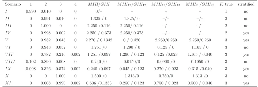
Table (2) gives the results of the simulation study in terms of the relative frequency, the marginal likelihood criterium chooses the corresponding number of clusters (1 through 4) for panel size A. Column 10 gives the true number of clusters. In Scenario I the marginal likelihood estimate for the true (pooled) model is in almost all cases higher than for the models with clusters. The model selection approach is at least well suited to reject the hypotheses of clustered data. If the simulated data is clustered the ability of the model selection approach to detect the right number of clusters is mixed and depends on the degree of homogeneity between the clusters and on whether one regards explaining variables for the (stratified) clustering.

(17)

Data in Scenarios II through IV are simulated from two clusters. In almost all cases the right number of clusters are estimated even when as in Scenario III and IV the heterogeneity between clusters is rather low. In ScenarioV three clusters exist, however the parametersβ are identical for two of them. Thus, these clusters are only different with respect to the logit part or the individuals in two of the three cluster behave like each other but for different reasons. The model selection can hardly detect the right number of clusters. It seems to be mainly driven by differences in β. In Scenarios V I and V II three clusters different inγ and β are assumed. However, the heterogeneity between two of theses clusters is rather low (M IH13= compare to scenario III). Again the model

selection procedure identifies only two clusters in most cases, but results improve if the conditioning information in the logit regression is taken into account. Thus it is advisable to do an one step analysis instead of a two step procedure, where in the first step clusters are estimated and in a second step logit parameters are estimated conditional on inferred states. This is even stressed in the assessment of ScenariosV III and IX where the heterogeneity between the β coefficients of the clusters is even lower, so that in a reasonable number of simulation runs (about 10 %) the marginal likelihood criterium even favors a pooled model in both scenarios. In ScenarioV III the true number of clusters is detected only in very few simulation runs due to the high similarity betweenβ1 andβ2

(M IH12= 0.015). In ScenarioIX when the logit specification is taken into account the number of

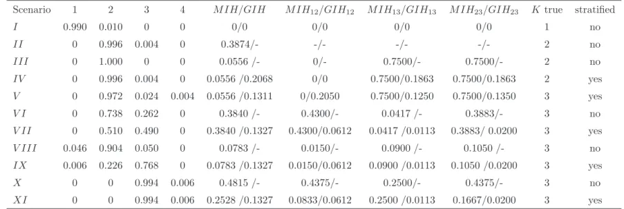
right model selections rises above 50 %. Finally, Scenarios X and XI provide an analysis for three rather heterogeneous cluster. Accordingly, the model selection procedure detects in almost all cases the true number of cluster. Qualitatively these results do not heavily depend on the structure of the data as the results for panel sizeB given in Table (3) show. They allow mainly the same conclusions as the results given for panel size A.

4.2 Cross validation approach

In this paragraph the results of the assessment of the marginal likelihood are compared to out-of-sample prediction criteria for model selection. We run an out-of-out-of-sample prediction exercises. The sample is spilt along time into an estimation sample containing 80 % of the observations of the whole sample while the remaining 20 % are to be forecasted. To expand the number of forecasts this partition (and thereby the forecasting exercise) is done five times in that way that all observations are once part of the forecasting sample. Results are averaged over this five different partitions.

Note that this approach allows the use of the unrestricted Gibbs-Sampler without application of relabeling to reach sensible results. In each Gibbs run we apply the set of sampled parameters on the covariates of the observations to be forecasted to obtain a forecast of the binary variable in each run.17

(18)

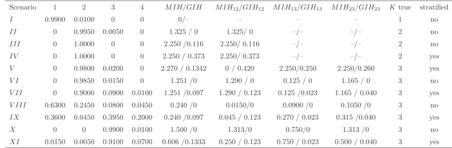
The forecasting distributions are thus byproducts of the Gibbs output. If the estimated probability exceeds 0.5, a one is taken as forecast for this observation and compared to the actually observed. Additionally, the ROC measure is calculated allowing for different probability borders in forecasting (hence, the popular approach with 0.5 is a special case of the ROC approach). The forecasts are done for the same models and scenarios as in the case of the marginal likelihood assessment. The number of clusters is then determined by the best model according to the forecasting and the ROC criterion respectively. Tables (4) and (6) report the relative frequencies the above explained criteria decide on the specific number of clusters in Panel size A.

Both, the forecasting and the ROC criterion provide very similar conclusions compared to the marginal likelihood. Thus the case of homogenity with no clusters is detected almost with certainty (scenario I). The same is true with two true clusters (scenarios II through IV) and with three true clusters if the heterogenity of the clusters is high enough (scenarios X and XI), whereby the marginal likelihood shows considerable less dispersion in the two latter scenarios. In scenarios V

through V II both criteria give advice to two clusters in more than 90 percent of the cases. While the marginal likelihood also has a high tendency to advice two clusters in these scenarios the rate of true selections is higher than for both competitors. Finally, in scenarios V II and IX the the most pronounced differences between the model selection criteria occur. The forecasting criterion has a high tendency to neglect the heterogeneity in 63 percent and 36 percent, respectively, it tends to just one cluster. The marginal likelihood and the ROC approach both have the same median: In scenario

V III both prefer two clusters mostly. Whereby the ROC approach has a higher dispersion. In 19 percent of the cases it chooses the right number of cluster, but in 26 percent of the cases it assumes just one clsuter and in 10 percent even four clusters. In scenarioIX the number of cases, where the true cluster dimension is detected is with 58 percent similar to the marginal likelihood approach, but here the ROC has a tendency to overfitting and more often signals four cluster. Tables (5) and (7) provide the results for Panel size B. Qualitatively the results are mainly unchanged. To some degree the dispersion of the decisions is a bit less and results are a bit improved in that sense for the ROC approach.

5 Empirical Illustration

The usefullness of model based clustering for modeling latent heterogeneity shall be illustrated using the data set studied in Bertschek and Lechner (1998). The data set is well known in the empirical literature and Greene (2004b) documents the presence of a considerable degree of latent heterogeneity within the data. The following listing gives the variables used for analysis, for a detailed description,

(19)

see Bertscheck and Lechner (1998):

yit= 1 if a product innovation was realized by firm iin year t, 0 otherwise;x2it Log of industry

sales in DM;x3itImport share=ratio of industry imports to (industry sales plus imports;x4itRelative

firm size = ratio of employment in business unit to employment in the industry (times 30);x5it FDI

share = Ratio of industry foreign direct investment to (industry sales plus imports);x6it Productivity

= Ratio of industry value added to industry employment;x7it Raw materials sector=1 if the firm is

in this sector; x8it Investment goods sector=1 if the firm is in this sector.

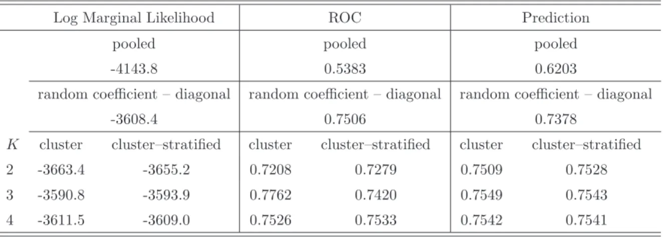
The data set contains 1270 firms, where the time dimension covers the five years from 1984 to 1988. Based on the insight delivered by the simulation study in the previous section, we consider the marginal likelihood analysis and the out-of-sample analysis with partitioning along the time dimension for determination of the number of latent clusters. The results are provided in Table (8). Comparison of the pooled specification with the specification incorporating random coefficients via the marginal likelihood shows the random coefficients specification to be very strongly preferred according to Jeffreys’ scale, see Jeffreys (1961). Consideration of latent heterogeneity via model based clustering asks for specifying the number of clusters. Table (8) gives the corresponding marginal likelihoods for models with two, three, and four clusters. For each number of cluster stratified and non stratified cluster specific probabilities have been considered. The marginal likelihood reveals that the consideration of three cluster in conjunction with non stratified cluster probabilities is the preferred model specification.

A similar conclusion is drawn on the basis of the performed out-of-sample prediction experiment. For both out-of-sample experiments with sample partitioning along the time dimension the ratio of correctly predicted observations and the ROC measure is the highest for the model specification incorporating latent heterogeneity via estimation of three latent clusters with non stratified cluster probabilities. Thus, also the empirical illustration provides evidence for the accuracy of the here proposed cross validation strategy for deciding on the preferred number of latent clusters.

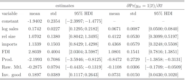
To reveal the impact of the considered forms of latent heterogeneity on gauging the impact of variables on the dependent variable firm innovation, we focus discussion on the implied different marginal effects. With respect to empirical results, Table (9) provides the pooled estimation results. All variables show significant influence on the dependent variable. Furthermore, marginal effects show that higher sales, larger size, higher import ratio and foreign direct investment, as well as membership in investment good branch have positive effect on the patent activity. Negative effects on patent activity are documented for productivity and the raw materials sector.

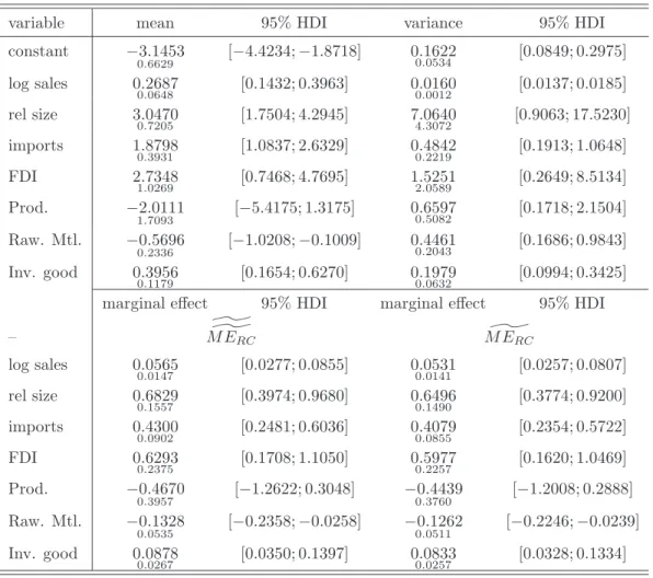
Incorporation of latent heterogeneity via random coefficients provides some significant changes with respect to the influence some variables exhibit on patent activity. Bayesian estimation results

(20)

are shown in Table (10).18 In specific, the productivity of a firm has no longer positive influence on the patent activity. The corresponding heterogeneity robust (in the sense of the random coefficient specification) marginal effect is not different from zero at conventional levels. The marginal effect for this specification using a numerical solution to the involved integral is computed as

^ ^ M ERC = 1 R R X r=1 1 N N X i=1 φ(xβ_i(r))β_i(r), (43)

where β_i(r), r = 1, . . . , R denote the posterior draws including the random coefficients. Using an analytical solution to the integration provides an estimate computed as

^ M ERC = 1 R R X r=1 exp{−.5(b(r)_′W−1,(r)_b(r)₎₋₍_W−1,(r)_b(r)₎_′_[_x′x₊_W−1,(r)_]−1₍_W−1,(r)_b(r)₎₎_} (2π)−.5det(W(r))−.5(det (x′x+W−1,(r))).5(x′x+W−1,(r))−1(W−1,(r)b(r)).(44) The estimation results corresponding to the estimation of three clusters are given in Table (11). Estimates are based on post screened Gibbs output. Figure (1) gives the posterior draws before post screening exhibit potentially multimodality and label switching. The post screened Gibbs output is given in Figure (2). It is seen that label switching has not been present in the Gibbs output, however slight genuine multi modality might be present, as shown in Figure (3) displaying the estimated posterior densities.19

With respect to empirical results, the preferred cluster specification provides an alternative ac-count of latent heterogeneity and recommends alternative interpretation of results. Consideration of latent heterogeneity via latent clusters allows to gain several insights with respect to the marginal ef-fects when latent heterogeneity is present. At first, cluster specific marginal efef-fects can be considered. These can be readily derived from the screened Gibbs output as

^ M EC = 1 R R X r=1 φ(xβ_k(r))β_k(r), k= 1, . . . , K (45)

and are based on cluster specific meansxk. However, generally no knowledge on cluster membership

is available. Therefore, of interest is also the distribution of marginal effects within the whole sample. Note that an heterogeneity robust average effect can be computed based on weighted averages of

18_{The random coefficient model has two blocks of parameters. The first block are the means of the random parameters}

and the second its variances. For the first block of parameters we assume a priori a multivariate normal distribution and for the second block we assume a Wishart distribution, the prior moments are given in Table (1). The Gibbs sampler is used to get inference on parameters and marginal effects.

19_{Numerical optimization routines to perform a Maximum Likelihood estimation yield differing results depending}

(21)

the draws given as ^ M ECR = 1 R R X r=1 K X k=1 w_k(r)φ(xβ_k(r))β_k(r), (46)

wherew_k(r)denotes the fraction of individuals in clusterkin Gibbs iterationr. Alternatively tow(_kr)

a conditional probability can be used, for example Pr(Si = k|x,{γ_k(r)}K_k₌₁−1). Draws of the cluster

specific marginal effects are hence weighted with the number of individuals, which are in this cluster for the considered draw. Table (12) gives the corresponding results.

While both, the random coefficient and the model-based clustering approach aim at a general representation of latent heterogeneity, several differences between the two specification are revealed, when comparing marginal effects. While within the population robust marginal effects given in Table (12) based on the latent cluster specification only log sales, relative firm size, and investment good sector have substantial influence on firm innovation, the random coefficient approach also exhibits substantial effect of imports and foreign direct investment. Furthermore, besides these qualitative differences, also quantitative differences for relative size and imports are revealed. In contrast very similar marginal effects are documented for log sales and the investment good sector indicator, see also the pooled specification in Table (9). These findings suggest that not all variables capture latent heterogeneity to the same extent. When looking at cluster specific marginal effects with estimation results being provided in Table (13), these provide insight into to what extent the clusters are distinct. Interestingly, within the cluster labeled as second all variables show substantial influence on firm innovation, however at a quantitative level differing from the pooled specification. For the first cluster only log sales and relative firm size are documented to have substantial impact, while for the third cluster log sales and the investment good sector influence firm innovation substantially. These different patterns provide insight into different latent cluster specific firm types, for which a pooled specification does not provide valid inference of the relationship between firm innovation and economic determinants thereof.

Given the latent cluster specification being the preferred model, comparison between cluster specific and random coefficient marginal effects suggests that the underlying normal distribution for latent heterogeneity does not allow to represent the full extent of the latent heterogeneity present within the considered empirical illustration. Thus, the empirical example reveals the importance to consider modeling latent heterogeneity in different manners.

6 Conclusion

This paper provides Bayesian estimation procedures for panel probit models incorporating model based clustering. Based on the different forms of incorporating latent heterogeneity, we provide

(22)

a discussion of different concepts of marginal effects. Furthermore, we discuss the issue of model selection with respect to the number of clusters. While the marginal likelihood is typically the preferred device for model selection in a Bayesian framework we propose the use of a cross-validation approach based on the ROC measure. The latter approach is less demanding than the marginal likelihood as it only needs the implementation of the Gibbs sampler and no further algorithms like the bridge sampler which is used for calculating the marginal likelihood. The results of a simulation study show that given the presence of a certain degree of inhomogeneity, both concepts correctly identifies the true number of latent clusters. Due to the high degree of complication in calculation marginal likelihoods for panel probit models the cross-validation approach seems to be a reasonable model selection tool. As a side result we find that stratified cluster probabilities perform overall better than non-stratified cluster probabilities, thus a one step procedure is preferred against possible two step procedures, where in a first step clusters are determined and in a second step a multinomial model is estimated.

Within the chosen empirical application we find strong evidence for latent heterogeneity captured via latent clusters. Based on the different forms of latent heterogeneity one arrives at different conclusions concerning the impact of explaining variables on the dependent variable conceptualized via marginal effects. This is a strong case for the class of models applied here and for the Bayesian approach to handle this class of models, as the Bayesian approach is able to deal with genuine multi modality and provides a consistent tool for model selection.

Acknowledgements

The authors thank Sylvia Fr¨uhwirth-Schnatter for helpful advice concerning the construction of the Rao-Blackwellized importance density and Roman Liesenfeld for thoughtful discussion.

(23)

References

[1] Albert, J. and S. Chib: 1993, ‘Bayesian Analysis of Binary and Polychotmous Response Data’. Journal of the American Statistical Association 88, 669–679.

[2] Andrews, D. W. K. and W. Ploberger: 1994, ‘Optimal Tests When a Nuisance Parameter Is Present Only under the Alternative’. Econometrica62(6), 1383–1414.

[3] Aßmann, C.: 2007, ‘Determinants and Costs of Current Account Reversals under Heterogeneity and Serial Correlation’. Economic Working Paper No. 2007-17, CAU Kiel.

[4] Ben-Akiva, M. and D. Bolduc: 1996, ‘Multinomial Probit with a logit kernel and a general parametric specification of the covariance structure’. Working paper, Department of Civil Engineering, MIT. [5] Bertschek, I. and M. Lechner: 1998, ‘Convenient estimators for the panel probit model’. Journal of

Econometrics87(2), 329–372.

[6] Cameron, C. and P. Trivedi: 2005,Microeconometrics: Methods and Applications. Cambridge University Press.

[7] Celeux, G.: 1998, ‘Bayesian inference for mixtures: the label switching problem’. COMPSTAT pp. 227–232.

[8] Chen, J. and A. Khalili: 2008, ‘Order Selection in Finite Mixture Models With a Nonsmooth Penalty’. Journal of the American Statistical Association 103(484), 1674–1683.

[9] Chib, S.: 1995, ‘Marginal Likelihood from the Gibbs output’. Journal of the American Statistical Asso-ciation 90(432), 1313–1321.

[10] Chib, S. and E. Greenberg: 1995, ‘Understanding the Metropolis-Hastings Algorithm’. The American Statistician49(4), 327–335.

[11] Chib, S. and I. Jeliazkov: 2001, ‘Marginal Likelihood from the Metropolis-Hastings Output’. Journal of the American Statistical Association96(453), 270–281.

[12] Dunson, D., A. Herring, and A. Siega-Riz: 2008, ‘Bayesian Inference on changes in response densities over predictor clusters’. Journal of the American Statistical Association 103(484), 1508–1517.

[13] Egan, J.: 1975,Signal Detection Theory and ROC analysis, Series in Cognition and Perception. Academic Press, New York.

[14] Fraley, C. and A. Raftery: 2002, ‘Model-Based Clustering, Discriminant Analysis, and Density Estima-tion’. Journal of the American Statistical Association97, 611–631.

[15] Fr¨uhwirth-Schnatter, S.: 2004, ‘Estimating marginal likelihoods for mixture and Markov switching mod-els using bridge sampling techniques’. The Econometrics Journal7, 143–167.

[16] Fr¨uhwirth-Schnatter, S. and S. Kaufmann: 2008, ‘Model-Based Clustering of Multiple Time Series’. Journal of Business & Economic Statistics26(1), 78–89.

(24)

[17] Geisser, S. and W. Eddy: 1979, ‘A predictive approach to model selection’. Journal of the American Statistical Association74(365), 153–160.

[18] Gelfand, A. E. and D. K. Dey: 1994, ‘Bayesian model choice: Asymptotics and exact calculations’. Journal of Royal Statistical Society B56, 501514.

[19] Gelfand, A. E. and A. Smith: 1990, ‘Sampling based approaches to calculating marginal densities’. Journal of the American Statistical Society85, 398–409.

[20] Greene, W.: 2004a, ‘The behaviour of the maximum likelihood estimator for limited dependent variable models in the presence of fixed effects’. Econometrics Journal7, 98–119.

[21] Greene, W.: 2004b, ‘Convenient estimators for the panel probit model: Further results’. Empirical Economics 29, 29–47.

[22] Greene, W. and D. Hensher: 2003, ‘A latent class model for discrete choice analysis: contrast to a mixed logit’. Transportation Research Part B37, 681–698.

[23] Handcock, M., A. E. Raftery, and J. Tantrum: 2007, ‘Model-based clustering for social networks’.Journal of the Royal Statistical Society A170(2), 301–354.

[24] Heard, N. A., C. C. Holmes, and D. A. Stephens: 2006, ‘A Quantitative Study of Gene Regulation Involved in the Immune Response of Anopheline Mosquitoes: An Application of Bayesian Hierarchical Clustering of Curves’. Journal of the American Statistical Society101(473), 18–29.

[25] Ishwaran, H., L. F. James, and J. Sun: 2001, ‘Bayesian Model Selection in Finite Mixtures by Marginal Density Decomposition’. Journal of the American Statistical Association 96(456), 1316–1332.

[26] Jeffreys, H.: 1961,Theory of probability. Oxford: Clarendon Press.

[27] Lancaster, T.: 2000, ‘The incidental parameter problem since 1948’. Journal of Econometrics95, 391– 413.

[28] Mehndiratta, S.: 1996, ‘Time-of-day effects in inter-city business travel’. Ph.D. thesis, University of California, Berkeley.

[29] Meng, X.-L. and W. H. Wong: 1996, ‘Simulating ratios of normalizing constants via a simple identity: A theoretical exploration’. Statistica Sinica6, 831860.

[30] Ray, S. and B. G. Lindsay: 2008, ‘Model selection in high dimensions: a quadratic-risk-based-approach’. Journal of the Royal Statistical Society, Series B70(1), 95–118.

[31] Revelt, D. and K. Train: 1998, ‘Mixed Logit with repeated choices’.Review of Economics and Statistics 80, 647–657.

[32] Stephens, M.: 2000, ‘Dealing with the label switching in mixture models’.Journal of the Royal Statistical Society B62(4), 795–809.

[33] Stone, M.: 1974, ‘Cross-validatory choice and assessment of statistical predictions’.Journal of the Royal Statistical Society B36, 111–147.

(25)

[34] Tanner, M. and W. Wong: 1987, ‘The calculation of posterior distributions by data augmentation’. Journal of the American Statistical Association 92(398), 528–540.

(26)

Tables

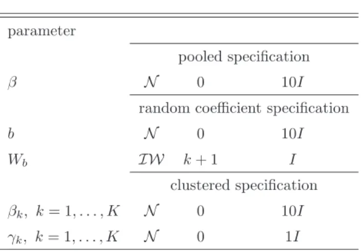
Table 1: Prior distributions

parameter

pooled specification

β N 0 10I

random coefficient specification

b N 0 10I

Wb IW k+ 1 I

clustered specification

βk, k= 1, . . . , K N 0 10I

(27)

Table 2: Simulation Study - Model selection via marginal likelihood - Panel size A

Scenario 1 2 3 4 M IH/GIH M IH12/GIH12 M IH13/GIH13 M IH23/GIH23 K true stratified

I 0.990 0.010 0 0 0/– – – – 1 no II 0 0.991 0.010 0 1.325 / 0 1.325/ 0 –/– –/– 2 no III 0 1.000 0 0 2.250 /0.116 2.250/ 0.116 –/– –/– 2 no IV 0 0.998 0.002 0 2.250 / 0.373 2.250/ 0.373 –/– –/– 2 yes V 0 0.952 0.048 0 2.270 / 0.1342 0 / 0.420 2.250/0.250 2.250/0.260 3 yes V I 0 0.948 0.052 0 1.251 /0 1.290 / 0 0.125 / 0 1.165 / 0 3 no V II 0 0.782 0.216 0.002 1.251 /0.097 1.290 / 0.123 0.125 /0.023 1.165 / 0.040 3 yes V III 0.102 0.890 0.008 0 0.240 /0 0.0150/0 0.0900 /0 0.1050 /0 3 no IX 0.098 0.326 0.574 0.002 0.240 /0.097 0.045 / 0.123 0.270 / 0.023 0.315 /0.040 3 yes X 0 0 1.000 0 1.500 /0 1.313/0 0.750/0 1.313 /0 3 no XI 0 0.008 0.990 0.002 0.606 /0.1333 0.250 / 0.123 0.750 / 0.023 0.500 / 0.040 3 yes

Notes: Simulation of 500 data sets for each scenario I–XI. Scenarios are described in Section xx. For each scenario the columns denotes the relative frequency the marginal likelihood decided for a specific number of clusters. Ktrue denotes the true number of clusters within the scenarios. IH denotes the inhomogeneity of the specified cluster specific parameters.

(28)

Table 3: Simulation Study - Model selection via marginal likelihood - Panel size B

I 0.990 0.010 0 0 0/0 0/0 0/0 0/0 1 no II 0 0.996 0.004 0 0.3874/- -/- -/- -/- 2 no III 0 1.000 0 0 0.0556 /- 0/- 0.7500/- 0.7500/- 2 no IV 0 0.996 0.004 0 0.0556 /0.2068 0/0 0.7500/0.1863 0.7500/0.1863 2 yes V 0 0.972 0.024 0.004 0.0556 /0.1311 0/0.2050 0.7500/0.1250 0.7500/0.1350 3 yes V I 0 0.738 0.262 0 0.3840 /- 0.4300/- 0.0417 /- 0.3883/- 3 no V II 0 0.510 0.490 0 0.3840 /0.1327 0.4300/0.0612 0.0417 /0.0113 0.3883/ 0.0200 3 yes V III 0.046 0.904 0.050 0 0.0783 /- 0.0150/- 0.0900 /- 0.1050 /- 3 no IX 0.006 0.226 0.768 0 0.0783 /0.1327 0.0150/0.0612 0.0900 /0.0113 0.1050 /0.0200 3 yes X 0 0 0.994 0.006 0.4815 /- 0.4375/- 0.2500/- 0.4375/- 3 no XI 0 0 0.994 0.006 0.2528 /0.1327 0.0833/0.0612 0.2500 /0.0113 0.1667/0.0200 3 yes

(29)

Table 4: Simulation Study - Model selection via Forecasting Criterion (T) - Panel size A

I 0.9900 0.0100 0 0 0/– – – – 1 no II 0 0.9950 0.0050 0 1.325 / 0 1.325/ 0 –/– –/– 2 no III 0 1.0000 0 0 2.250 /0.116 2.250/ 0.116 –/– –/– 2 no IV 0 1.0000 0 0 2.250 / 0.373 2.250/ 0.373 –/– –/– 2 yes V 0 0.9800 0.0200 0 2.270 / 0.1342 0 / 0.420 2.250/0.250 2.250/0.260 3 yes V I 0 0.9850 0.0150 0 1.251 /0 1.290 / 0 0.125 / 0 1.165 / 0 3 no V II 0 0.9000 0.0900 0.0100 1.251 /0.097 1.290 / 0.123 0.125 /0.023 1.165 / 0.040 3 yes V III 0.6300 0.2450 0.0800 0.0450 0.240 /0 0.0150/0 0.0900 /0 0.1050 /0 3 no IX 0.3600 0.0450 0.3950 0.2000 0.240 /0.097 0.045 / 0.123 0.270 / 0.023 0.315 /0.040 3 yes X 0 0 0.9900 0.0100 1.500 /0 1.313/0 0.750/0 1.313 /0 3 no XI 0.0150 0.0050 0.9100 0.0700 0.606 /0.1333 0.250 / 0.123 0.750 / 0.023 0.500 / 0.040 3 yes

(30)

Table 5: Simulation Study - Model selection via Forecasting Criterion (T) - Panel size B

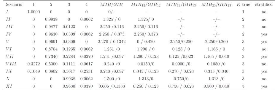
I 1.0000 0 0 0 0/– – – – 1 no II 0 0.9938 0 0.0062 1.325 / 0 1.325/ 0 –/– –/– 2 no III 0 0.9877 0.0123 0 2.250 /0.116 2.250/ 0.116 –/– –/– 2 no IV 0 0.9630 0.0309 0.0062 2.250 / 0.373 2.250/ 0.373 –/– –/– 2 yes V 0 0.9691 0.0309 0 2.270 / 0.1342 0 / 0.420 2.250/0.250 2.250/0.260 3 yes V I 0 0.8704 0.1235 0.0062 1.251 /0 1.290 / 0 0.125 / 0 1.165 / 0 3 no V II 0 0.7346 0.2284 0.0370 1.251 /0.097 1.290 / 0.123 0.125 /0.023 1.165 / 0.040 3 yes V III 0.3272 0.5000 0.1111 0.0617 0.240 /0 0.0150/0 0.0900 /0 0.1050 /0 3 no IX 0.1049 0.0802 0.5617 0.2531 0.240 /0.097 0.045 / 0.123 0.270 / 0.023 0.315 /0.040 3 yes X 0 0 0.9938 0.0062 1.500 /0 1.313/0 0.750/0 1.313 /0 3 no XI 0 0 0.9630 0.0370 0.606 /0.1333 0.250 / 0.123 0.750 / 0.023 0.500 / 0.040 3 yes

(31)

Table 6: Simulation Study - Model selection via ROC Graph - Panel size A

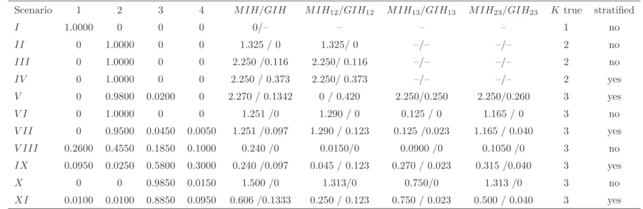
I 1.0000 0 0 0 0/– – – – 1 no II 0 1.0000 0 0 1.325 / 0 1.325/ 0 –/– –/– 2 no III 0 1.0000 0 0 2.250 /0.116 2.250/ 0.116 –/– –/– 2 no IV 0 1.0000 0 0 2.250 / 0.373 2.250/ 0.373 –/– –/– 2 yes V 0 0.9800 0.0200 0 2.270 / 0.1342 0 / 0.420 2.250/0.250 2.250/0.260 3 yes V I 0 1.0000 0 0 1.251 /0 1.290 / 0 0.125 / 0 1.165 / 0 3 no V II 0 0.9500 0.0450 0.0050 1.251 /0.097 1.290 / 0.123 0.125 /0.023 1.165 / 0.040 3 yes V III 0.2600 0.4550 0.1850 0.1000 0.240 /0 0.0150/0 0.0900 /0 0.1050 /0 3 no IX 0.0950 0.0250 0.5800 0.3000 0.240 /0.097 0.045 / 0.123 0.270 / 0.023 0.315 /0.040 3 yes X 0 0 0.9850 0.0150 1.500 /0 1.313/0 0.750/0 1.313 /0 3 no XI 0.0100 0.0100 0.8850 0.0950 0.606 /0.1333 0.250 / 0.123 0.750 / 0.023 0.500 / 0.040 3 yes

(32)

Table 7: Simulation Study - Model selection via ROC Graph - Panel size B

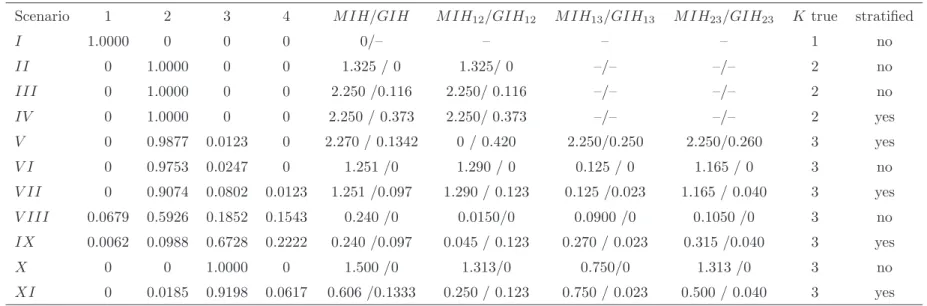
I 1.0000 0 0 0 0/– – – – 1 no II 0 1.0000 0 0 1.325 / 0 1.325/ 0 –/– –/– 2 no III 0 1.0000 0 0 2.250 /0.116 2.250/ 0.116 –/– –/– 2 no IV 0 1.0000 0 0 2.250 / 0.373 2.250/ 0.373 –/– –/– 2 yes V 0 0.9877 0.0123 0 2.270 / 0.1342 0 / 0.420 2.250/0.250 2.250/0.260 3 yes V I 0 0.9753 0.0247 0 1.251 /0 1.290 / 0 0.125 / 0 1.165 / 0 3 no V II 0 0.9074 0.0802 0.0123 1.251 /0.097 1.290 / 0.123 0.125 /0.023 1.165 / 0.040 3 yes V III 0.0679 0.5926 0.1852 0.1543 0.240 /0 0.0150/0 0.0900 /0 0.1050 /0 3 no IX 0.0062 0.0988 0.6728 0.2222 0.240 /0.097 0.045 / 0.123 0.270 / 0.023 0.315 /0.040 3 yes X 0 0 1.0000 0 1.500 /0 1.313/0 0.750/0 1.313 /0 3 no XI 0 0.0185 0.9198 0.0617 0.606 /0.1333 0.250 / 0.123 0.750 / 0.023 0.500 / 0.040 3 yes

(33)

Table 8: Model Comparison – Log Marginal Likelihood and Out-of-Sample Prediction

Log Marginal Likelihood ROC Prediction pooled pooled pooled -4143.8 0.5383 0.6203

random coefficient – diagonal random coefficient – diagonal random coefficient – diagonal -3608.4 0.7506 0.7378

K cluster cluster–stratified cluster cluster–stratified cluster cluster–stratified 2 -3663.4 -3655.2 0.7208 0.7279 0.7509 0.7528 3 -3590.8 -3593.9 0.7762 0.7420 0.7549 0.7543 4 -3611.5 -3609.0 0.7526 0.7533 0.7542 0.7541

(34)

Table 9: Pooled Specification

estimates ∂Pr(yit= 1|x)/∂x

variable mean std 95% HDI mean std 95% HDI constant -1.9402 0.2354 [−2.3997;−1.4775] – – – log sales 0.1742 0.0227 [0.1295; 0.2182] 0.0671 0.0087 [0.0500; 0.0840] rel size 1.0702 0.1380 [0.8042; 1.3495] 0.4122 0.0530 [0.3099; 0.5197] imports 1.1339 0.1503 [0.8429; 1.4298] 0.4368 0.0579 [0.3248; 0.5508] FDI 2.8039 0.4004 [2.0304; 3.5987] 1.0801 0.1541 [0.7816; 1.3851] Prod. -2.1993 0.7086 [−3.5946;−0.8125] -0.8472 0.2729 [−1.3858;−0.3131] Raw. Mtl. -0.2875 0.0794 [−0.4435;−0.1319] -0.1108 0.0306 [−0.1709;−0.0509] Inv. good 0.1897 0.0389 [0.1117; 0.2643] 0.0731 0.0150 [0.0430; 0.1020]

(35)

Table 10: Random Coefficient Specification – diagonal

variable mean 95% HDI variance 95% HDI constant −3.1453 0.6629 [−4.4234;−1.8718] 00..16220534 [0.0849; 0.2975] log sales 0.2687 0.0648 [0.1432; 0.3963] 00..01600012 [0.0137; 0.0185] rel size 3.0470 0.7205 [1.7504; 4.2945] 74..06403072 [0.9063; 17.5230] imports 1.8798 0.3931 [1.0837; 2.6329] 00..48422219 [0.1913; 1.0648] FDI 2.7348 1.0269 [0.7468; 4.7695] 12..52510589 [0.2649; 8.5134] Prod. −2.0111 1.7093 [−5.4175; 1.3175] 00..65975082 [0.1718; 2.1504] Raw. Mtl. −0.5696 0.2336 [−1.0208;−0.1009] 00..44612043 [0.1686; 0.9843] Inv. good 0.3956 0.1179 [0.1654; 0.6270] 00..19790632 [0.0994; 0.3425]

marginal effect 95% HDI marginal effect 95% HDI – M E^^RC M E^RC log sales 0.0565 0.0147 [0.0277; 0.0855] 00..05310141 [0.0257; 0.0807] rel size 0.6829 0.1557 [0.3974; 0.9680] 00..64961490 [0.3774; 0.9200] imports 0.4300 0.0902 [0.2481; 0.6036] 00..40790855 [0.2354; 0.5722] FDI 0.6293 0.2375 [0.1708; 1.1050] 00..59772257 [0.1620; 1.0469] Prod. −0.4670 0.3957 [−1.2622; 0.3048] −00.3760.4439 [−1.2008; 0.2888] Raw. Mtl. −0.1328 0.0535 [−0.2358;−0.0258] −00.0511.1262 [−0.2246;−0.0239] Inv. good 0.0878 0.0267 [0.0350; 0.1397] 00..08330257 [0.0328; 0.1334]

(36)

Table 11: Parameter Estimates Cluster Specification – K = 3

k= 1 k= 2 k= 3

variable mean / std 95% HDI mean / std 95% HDI mean / std 95% HDI constant −2.0456 0.7034 [−3.4881;−0.7273] −02..73404621 [−3.8931;−1.0214] −16..49343776 [−9.8281;−3.8364] log sales 0.2650 0.0706 [0.1315; 0.4092] 00..16610659 [0.0353; 0.2937] 00..36011227 [0.1375; 0.6265] rel size 4.6454 1.0988 [2.8024; 7.1186] 00..87934529 [0.1927; 2.0339] 10..23756160 [0.1941; 2.5098] imports 0.8145 0.4472 [−0.0596; 1.6886] 20..23865168 [1.2560; 3.2895] 11..56183235 [−1.3657; 3.6694] FDI 1.1766 1.4908 [−1.7619; 4.2059] 21..26703647 [0.1173; 5.7940] 32..27799830 [−3.6103; 7.9629] Prod. −1.0736 2.6381 [−6.0471; 4.0568] −21..54246256 [−7.3004; 1.9024] 02..13372981 [−4.5534; 5.2717] Raw. Mtl. −0.3785 0.2245 [−0.8244; 0.0430] −00..39099065 [−1.7077;−0.2057] 01..61091467 [−2.5092; 2.8301] Inv. good 0.1725 0.1274 [−0.0830; 0.4233] 00..43551291 [0.1833; 0.6896] 00..75985579 [0.1884; 2.8471] γ1/γ2/γ3 0.4597 0.0449 [0.3687; 0.5441] 00..33870385 [0.2640; 0.4144] 00..20160340 [0.1316; 0.2666] 33

(37)

Table 12: Marginal Effects in Population

marginal effect 95% HDI constant – – log sales 0.0550 0.0183 [0.0193; 0.0898] rel size 0.1922 0.0955 [0.0362; 0.3861] imports 0.2712 0.1665 [−0.0654; 0.5680] FDI 0.6361 0.4553 [−0.3405; 1.4273] Prod. 0.0023 0.3433 [−0.6755; 0.8056] Raw. Mtl. 0.1102 0.1152 [−0.0944; 0.3345] Inv. good 0.0922 0.0330 [0.0293; 0.1581]

(38)

Table 13: Cluster Specific Marginal Effects –K = 3

k= 1 k= 2 k= 3

variable mean / std 95% HDI mean / std 95% HDI mean / std 95% HDI constant −0.3157 0.1082 [−0.5234;−0.1017] −00..28619766 [−1.5493;−0.4234] −00..28705672 [−1.0147;−0.0500] log sales 0.0406 0.0112 [0.0186; 0.0619] 00..06350252 [0.0147; 0.1129] 00..03200182 [0.0017; 0.0644] rel size 0.7132 0.1190 [0.4770; 0.9391] 00..34421652 [0.0925; 0.7422] 00..11350790 [−0.0148; 0.2680] imports 0.1280 0.0675 [−0.0010; 0.2660] 00..89211879 [0.5253; 1.2609] 00..15571347 [−0.0593; 0.4086] FDI 0.1886 0.2135 [−0.2018; 0.6451] 00..85805052 [0.0491; 2.0094] 00..30233551 [−0.2702; 1.0138] Prod. −0.1921 0.4089 [−1.0165; 0.5783] −00..94905491 [−2.7600; 0.7454] 00..01932293 [−0.4603; 0.5594] Raw. Mtl. −0.0562 0.0305 [−0.1179; 0.0043] −00..14303319 [−0.6459;−0.0837] 00..03640959 [−0.1945; 0.2123] Inv. good 0.0276 0.0187 [−0.0091; 0.0638] 00..17240478 [0.0787; 0.2660] 00..06140285 [0.0113; 0.1192] 35

(39)

Figures

0 1 2 x 104 −6 −5 −4 −3 −2 −1 0 1 K=1 0 1 2 x 104 −0.1 0 0.1 0.2 0.3 0.4 0.5 0.6 0 1 2 x 104 0 2 4 6 8 10 0 1 2 x 104 −2 −1 0 1 2 3 0 1 2 x 104 −6 −4 −2 0 2 4 6 8 0 1 2 x 104 −15 −10 −5 0 5 10 0 1 2 x 104 −2 −1.5 −1 −0.5 0 0.5 1 0 1 2 x 104 −0.6 −0.4 −0.2 0 0.2 0.4 0.6 0.8 0 1 2 x 104 −6 −4 −2 0 2 K=2 0 1 2 x 104 −0.2 −0.1 0 0.1 0.2 0.3 0.4 0.5 0 1 2 x 104 −2 −1 0 1 2 3 4 0 1 2 x 104 0 1 2 3 4 5 0 1 2 x 104 −5 0 5 10 15 0 1 2 x 104 −15 −10 −5 0 5 10 0 1 2 x 104 −3 −2 −1 0 1 0 1 2 x 104 −0.2 0 0.2 0.4 0.6 0.8 1 1.2 0 1 2 x 104 −15 −10 −5 0 K=3 0 1 2 x 104 −0.2 0 0.2 0.4 0.6 0.8 1 1.2 0 1 2 x 104 −5 0 5 0 1 2 x 104 −10 −5 0 5 10 0 1 2 x 104 −15 −10 −5 0 5 10 15 0 1 2 x 104 −15 −10 −5 0 5 10 15 0 1 2 x 104 −10 −5 0 5 10 0 1 2 x 104 −1 0 1 2 3 4 5