Sharif University of Technology
Scientia Iranica
Transactions A: Civil Engineering www.sciencedirect.com
Reliable pavement backcalculation with confidence estimation
K. Gopalakrishnan
a,∗,
H. Papadopoulos
baDepartment of Civil, Construction and Environmental Engineering, Iowa State University, Ames, IA 50011, USA bDepartment of Computer Science and Engineering, Frederick University, Nicosia 1036, Cyprus
Received 1 August 2011; revised 6 September 2011; accepted 1 November 2011
KEYWORDS Confidence machine; Conformal prediction; Hedging; Pavement; Backcalculation; Inverse analysis; Falling weight deflectometer.
Abstract Conformal Prediction (CP) is a novel machine learning concept which uses past experience to determine precise levels of confidence in new predictions. Traditional machine learning algorithms, such as Neural Networks (NN), Support Vector Machines (SVM), etc. output simple, bare predictions without an indication (confidence) of how likely each prediction is of being correct. However, in real-world problem domains, it is highly desirable to have predictions complemented with a tolerance interval to assess their credibility and accuracy. CP can be thought of as a strategy built on top of a machine learning algorithm to hedge its predictions with valid confidence. In this paper, a NN Regression (NNR) model is used to derive a decision rule for the inverse prediction of non-linear pavement layer moduli from Non-Destructive Test (NDT) deflection data. A CP is then implemented for the NNR decision rule and tested on an independent data set to demonstrate its error calibration properties. It is shown that CP can be used to derive reliable pavement moduli predictions without compromising the accuracy of the NNR decision rule but with control of the risk of error.
©2012 Sharif University of Technology. Production and hosting by Elsevier B.V.
1. Introduction
1.1. Problem description
Pavement engineers diagnose the structural condition of roads by conducting a Non-Destructive Test (NDT) and deter-mining the moduli or stiffness of pavement layers from NDT de-flection data through an inverse process (typically referred to as backcalculation). The Falling Weight Deflectometer (FWD) test is the most commonly employed NDT, which simulates a load pulse induced by a truck moving at moderate speeds, and mea-sures the deflections in the pavement using sensors radiating from a loading plate attached to the test device. The pavement
∗Corresponding author.
E-mail address:[email protected](K. Gopalakrishnan).
layer stiffness determined through inverse analysis is a relative indicator of pavement condition, and is also used in estimating the remaining life of the pavement and in the design of pave-ment rehabilitation alternatives.
In recent years, several Artificial Intelligence (AI) based techniques have been proposed for the inverse analysis of pavement systems [1], starting with the use of Neural Networks (NN) for predicting pavement layer moduli from synthetically generated pavement deflection basins using an elastic layered analysis [2]. More recently, Ceylan et al. [3] reported on the development of a comprehensive suite of NN models for the prediction of nonlinear, stress-dependent pavement layer moduli from a Finite Element (FE) generated synthetic database.
But, so far, all AI methods developed for the prediction of pavement layer moduli from NDT data yield only a ‘bare’ predictive value, and do not report on the credibility and accuracy of information. Without knowing the confidence of predictions, it is difficult to measure and control the risk of error associated with the predictions. Thus, decisions cannot be taken rationally unless this uncertain nature of the problem domain is taken into account. For instance, in weather forecasting, the Probability of Precipitation figures are more commonly used rather than simple bare predictions of ‘rain’ or ‘no rain’ [4]. This is also true in forecasting structural failures or in the non-destructive assessment of pavement systems where levels of misdiagnosis risk need to be understood.
1026-3098©2012 Sharif University of Technology. Production and hosting by
doi:10.1016/j.scient.2011.11.018
Open access under CC BY-NC-ND license.
Elsevier B.V.
Peer review under responsibility of Sharif University of Technology.
1.2. Conformal prediction
Conformal Prediction (CP) provides a promising framework that yields prediction coupled with confidence estimation [5–10]. When predictions are made with confidence, it has to be ensured that they are reliable by matching the forecast levels of confidence with the actual outcome [11]. For instance, in the same example of weather forecasting, if the actual frequency of outcome is approximately greater or equal to the forecasting level of confidence, say 95%, then the forecaster is said to be well-calibrated.
CP is theoretically founded on the algorithmic randomness theory and provides provably valid confidence measures based only on the assumption that the data in question are identically and independently distributed (i.i.d.). It has been shown to be well-calibrated for on-line learning [7]. It has also been demonstrated as well-calibrated empirically for several off-line learning problems [4]. A useful property of CP is that it allows direct control of the risk of prediction error by calibration to a specified confidence level. This is made possible due to its ability to make hedged or uncertain predictions to achieve a higher probability of success.
Conformal Predictors (CPs) are built on top of standard Machine Learning algorithms (referred to as underlying algo-rithms) used for outputting bare predictions. To date, many CPs have been developed based on popular conventional al-gorithms, such as Support Vector Machines [5,12], k-Nearest Neighbours [13], Neural Networks [14], Evolutionary Algo-rithms [15], Ridge Regression [16], k-Nearest Neighbours Regression [17] and Neural Networks Regression [17]. Some examples of real life problems, where CPs have been applied successfully, are classification of leukaemia subtypes [4], early detection of ovarian cancer [18], diagnosis of acute abdom-inal pain [19], assessment of stroke risk [20], prediction of plant promoters [21] and the estimation of effort for software projects [22].
The Transductive Conformal Prediction (TCP) approach, originally developed by Gammerman et al. [5], and some of its variants have, in general, the disadvantage of being computa-tionally inefficient. Saunders et al. [23] as well as Gammerman and Vovk [6] proposed much more efficient versions of TCP. Papadopoulos et al. [24,25] introduced Inductive Conformal Prediction (ICP), a computationally efficient CP approach for re-gression and classification, respectively, which performs induc-tive instead of transducinduc-tive inference. The biggest advantage of ICP is that it is as efficient as the corresponding underlying al-gorithm [14].
In this paper, a Neural Networks Regression ICP (NNR-ICP) approach is developed for making hedged predictions of pavement layer moduli with predefined confidence levels. In contrast to the original NNR method, which outputs ‘bare’ predictions of pavement layer moduli, every prediction output by NNR-ICP is a set of possible values denoted as the ‘prediction region’ or ‘prediction interval’ (also known as the tolerance interval) from which the credibility and accuracy of pavement layer moduli predictions can be estimated. Although numerous AI-based pavement moduli inverse methodologies have been developed in the past, this is the first time the risk of prediction error is understood and possibly controlled, which has practical implications in the context of mechanistic-based pavement analysis and design.
2. Neural Networks Regression (NNR) inverse pavement moduli prediction model: underlying algorithm
This study will focus on flexible pavement systems. A typical three-layered flexible pavement structure consists of a Hot-Mix
Asphalt (HMA) surface layer, a granular base layer consisting of unbound aggregates, and the bottommost layer consisting of subgrade soils.
The Elastic Layered Programs (ELPs) used in the analysis and design of flexible pavements consider the pavement as an elas-tic multi-layered media, and assume that pavement materi-als are linear-elastic, homogeneous and isotropic. However, the unbound granular materials and fine-grained subgrade soils, referred to as pavement geomaterials, do not follow a lin-ear stress–strain behavior under repeated traffic loading. The non-linearity or stress-dependency of resilient modulus for un-bound granular materials and cohesive fine-grained subgrade soils has been well established [26,27]. Unbound aggregates exhibit a stress hardening type behavior whereas fine-grained subgrade soils show a stress-softening type behavior.
2.1. Neural Networks Regression (NNR) methodology
Over the years, NNs have emerged as successful computa-tional tools for studying a majority of pavement engineering problems [1,2,28]. In the development of the mechanistic-empirical pavement design guide for the American Associa-tion of State Highway and TransportaAssocia-tion Officials (AASHTO), NNs have been recognized as non-traditional yet very power-ful, computing techniques and were used in preparing the con-crete pavement analysis package. Recent research studies at Iowa State University have focused on the development of NN based forward and backcalculation type highway flexible pave-ment analysis models to predict critical pavepave-ment responses and layer moduli, respectively [2].
The basic element in Neural Networks is a processing ele-ment (artificial neuron). An artificial neuron receives informa-tion (signal) from other neurons, processes it, and then relays the filtered signal to the other neurons [29]. The receiving end of the neuron has incoming signals, in1
,
in2, . . . ,
inn. Each of them is assigned a weight, which is given based on experience and which may change during the training process. The summa-tion of all weighted signal amounts yields the combined input quantity,Ik. The combined input quantity,Ik, is then sent to a pre-selected transfer function (sometimes called an activation function),T, and a filtered output,ok, is generated in the outgo-ing end of the artificial neuron,k, through the mapping of the transfer function. The process can be written in the form of the following equations: Ik=
n
i=1w
ikini,
(1) ok=
T(
I).
(2)There are several types of transfer function that can be used, including sigmoid, threshold and Gaussian functions. The transfer function most often used is the sigmoid function. The sigmoid function can be represented by the following equation: T
(
I)
=
11
+
exp(
−
ϕ
I)
,
(3)where
ϕ
=
positive scaling constant, which controls the steepness between the two asymptotic values, 0 and 1 [29]. The Backpropagation(BP) learning algorithm is the most commonly used NN training algorithm in which the network learns the relationship between stipulated input–output data pairs in a supervised manner. In the BP learning algorithm, the error energy used for monitoring the progress toward convergence is the generalized value of all errors, which is calculated by the least-squares formulation, and represented by a Mean Squared Error (MSE) as follows [30]:MSE
=
1 MP p
1 m
k=1(
dk−
yk)
2,
(4)whereykanddkare actual and desired outputs, respectively,M is the number of neurons in the output layer andPrepresents the total number of training patterns. Other performance measures, such as the Cross-Entropy Error (CE), Root Mean Squared Error (RMSE), Average Absolute Error (AAE), etc. are also used.
2.2. Data set generation
A multilayer feedfoward Neural Network with a BP learning algorithm was employed in developing an inverse pavement layer prediction model. The goal is to simulate FWD loading, using a numerical model for a wide variety of layer thicknesses and combinations of layer moduli encountered in the field, resulting in a comprehensive synthetic solution set. A 2-D axi-symmetric FE program (Raad and Figueroa 1980) developed at the University of Illinois and commonly used in the structural analysis of flexible pavements was employed to generate a comprehensive synthetic database of moduli-deflection solutions for wide ranges of layer thickness and layer moduli. Numerous research studies have validated that the FE model [31] used in this study provides a realistic pavement structural response prediction for both highway and airfield pavements by incorporating stress-sensitive geo-material models, the typical hardening behaviour of nonlinear unbound aggregate bases, the softening nature of subgrade soils under increasing stress states, and Mohr-Coulomb failure criteria to limit material strength.
The synthetic database of FE solutions constituted the training and testing sets for developing NNR-based models for the rapid inverse prediction of flexible pavement layer moduli. A generic three-layer flexible pavement structure consisting of a HMA surface layer, an unbound aggregate base layer, and a subgrade layer was modeled using the FE software. The top surface HMA layer was characterized as a linear elastic material with Young’s Modulus, EHMA, and Poisson ratio,
ν
. The K–θ
model [32] was used as the non-linear characterization model for the unbound aggregate layer:ER
=
K(θ/
po)
n,
(5)whereER is resilient modulus (MPa),
θ
=
σ
1+
σ
2+
σ
3=
σ
1+
2σ
3=
bulk stress,pois the unit reference pressure (1 kPa or 1 psi) used in the model to make the stresses non-dimensional, andK andnare multiple regression constants obtained from repeated load triaxial test data on granular materials. Based on the work reported by Rada and Witczak [33],K andnmodel parameters can be correlated to characterize the non-linear stress dependent behavior with only one model parameter. Thus, good quality granular materials, such as crushed stone, show higherKand lowernvalues whereas the opposite applies for lower quality aggregates.Fine-grained subgrade soils were modeled using the com-monly used bilinear resilient modulus model [27]:
ER
=
ERi=
K1·
(σ
d−
σ
di)
forσ
d< σ
diER
=
ERi=
K2·
(σ
d−
σ
di)
forσ
d> σ
di,
(6)where ERi is the ‘‘breakpoint’’ resilient modulus,
σ
d is the breakpoint deviator stress(σ
d=
σ
1−
σ
3), σ
diis the breakpoint deviator stress, and K1 and K2 are statistically determined coefficients from laboratory tests.ERi can be used to classify fine-grained subgrade soils as being soft, medium or stiff.Based on extensive repeated laboratory testing data at the University of Illinois, Thompson and Robnett [34] indicated that ERi, typically associated with a repeated deviator stress of about 41 kPa (6 psi), is a good indicator of the subgrade soil’s resilient modulus.
Thus, HMA modulus, EHMA, granular base K–
θ
model parameterK, and the subgrade break-point resilient moduli, ERi, were used as the layer stiffness inputs for all the FE runs. A 40 kN wheel load was applied at a uniform pressure of 552 kPa over a circular area of radius 150 mm simulating the FWD loading. A comprehensive FE synthetic database was generated by varying the HMA layer thickness (in the range of 75–400 mm), aggregate base layer thickness (in the range of 100–550 mm),EHMA (in the range of 6.9–41.5 GPa),K (in the range of 21–82 MPa) andERi(in the range of 7–105 MPa) for NN training and testing. The ranges of pavement layer properties used in developing the FE synthetic database are summarized inTable 1. Independent datasets were used for NN training and testing. The training dataset was comprised of 28,000 records and an independent set of 1500 records were used for testing the developed NN models.Several network architectures with two hidden layers were trained. Overall, the training and testing Mean Squared Errors (MSEs) decreased as the networks grew in size with an increasing number of neurons in the hidden layers. The error levels for both the training and testing sets matched closely when the number of hidden nodes approached 60.
2.3. Final decision rule
In this study, the 8-60-60-1 architecture (8 inputs, two hidden layers with 60 neurons each and 1 output) was chosen as the best architecture for the NNR inverse model based on its lowest training and testing Mean Squared Errors (MSEs) in the order of 1
×
10−4(corresponding to a Root Mean Squared Error ([RMSE) of 0.3%) for both output variables, HMA layer moduli (EHMA) and non-linear subgrade layer moduli (ERi). Separate NN models were developed for predicting each of the pavement layer moduli.The eight inputs in the best-performance NNR architec-ture (8-60-60-1) include the six FWD surface deflections (D0
,
D300,
D600,
D900,
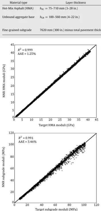
D1200andD1500) measured at the load drop location (0 mm) and at radial offsets of 300 mm (12 in.), 600 mm (24 in.), 900 mm (36 in.), 1200 mm (48 in.) and 1500 mm (60 in.), and two known pavement layer thicknesses: HMA layer (hAC) and the unbound granular base layer (hGB).Figure 1 depicts the prediction ability of the 8-60-60-1 network at the 10,000th training epoch. Average Absolute Errors (AAEs) were calculated as the sum of the individual absolute errors divided by the 1500 independent testing patterns. The AAE for the HMA layer moduli was a low 1.25% while the AAE for the subgrade breakpoint moduli,ERi, was 3.46%. Note that the HMA moduli is strongly related to the maximum FWD surface deflection, D0, while the subgrade moduli is largely a function of FWD surface deflection at offsets greater than 914 mm (36 in.). Note that the magnitude of FWD surface deflections decreases with increasing radial offsets and so does the relative accuracy of measurements. As a result, the prediction accuracy for HMA moduli is generally higher compared to subgrade moduli.
As shown inFigure 1, almost all 1500 NNR predictions fell on the line of equality for the two pavement layer moduli, thus, indicating the proper training and excellent performance of the NNR models. The development of NN inverse prediction models employed in this study are discussed in detail by Gopalakrishnan et al. [35].
Table 1: Pavement geometry and material property/model inputs of flexible pavement systems for ILLI-PAVE solutions.
Material type Layer thickness Material model Layer modulus inputs Hot-Mix Asphalt (HMA) hAC=75–710 mm (3–28 in.) Linear elastic EAC=6.9–41.4 GPa (100–6000 ksi)
Unbound aggregate base hGB=100–560 mm (4–22 in.) NonlinearK–θmodel
MR=Kθn
‘‘K’’=20–83 MPa (3–12 ksi) ‘‘n’’ from Eq.(5)
Fine-grained subgrade 7620 mm (300 in.) minus total pavement thickness Nonlinear bilinear Model MR=f(ERi);
ERi=1–15 ksi
Figure 1: Prediction performance of underlying algorithm (NN backcalculation models). (a) HMA moduli; and (b) subgrade moduli.
3. NNR-ICP approach to pavement inverse analysis
In the previous section, the development of the final decision rule for NN-based inverse moduli predictions was discussed. The next step is to develop the ICP model over the induction NNR decision rule referred to as the NNR-ICP model. For this, a calibration dataset was selected independent of training and testing datasets from the synthetic database.Figure 2illustrates the schematic of the NNR-ICP model, which will be used for making calibrated region predictions.
The NNR-ICP approach uses the calibration set and the derived NNR rule to calculate thep-values of all possible labels
of the new example. Thesep-values are used to compute well-calibrated region predictions, which allow hedged pavement moduli predictions to be made.
3.1. NNR-ICP algorithm
The NNR-ICP algorithm proposed by Papadopoulos and Haralambous [17] is adapted here for developing the NNR-ICP pavement backcalculation algorithm:
1. Let the proper training set and the calibration set be represented as:
Proper training set:
{
(
x1,
y1) , (
x2,
y2) , . . . , (
xm,
ym)
}
where m<
l.Calibration set:
{
(
xm+1,
ym+1) , (
xm+2,
ym+2) , . . . , (
xl,
yl)
}
withk=
l−
melements.2. A nonconformity score or strangeness value is associated with every pair
(
xm+i,
ym+i)
in the calibration set using what is called anonconformity measure. The nonconformity measure evaluates how strange the pair is for the trained NNR rule. This measure can be defined as:α
i=
ym+i− ˆ
ym+i
i=
1,
2, . . . ,
k,
(7)wherey
ˆ
m+iis the prediction value given by the underlying NNR algorithm.3. Accordingly, the nonconformity score for every potential label,y, of the new unlabelled example,xl+1, can be defined as:
α
l+1=
y− ˆ
yl+1
,
(8)wherey
ˆ
l+1is the prediction given by the derived rule for the new example.4. Then, thep-value associated with the potential label,y, is defined as:
p
(
y)
=
#{
i=
m+
1, . . . ,
m+
k,
l+
1:
α
i≥
α
l+1}
k
+
1,
(9)where #Astands for the number of elements of setA. A proof that thep
(
y)
calculated by Eq.(9)are validp-values, is given by Papadopoulos et al. [24].5. Suppose some confidence level, 1
−
δ
, is given a priori whereδ >
0 is a small constant (e.g. 1% or 5%) called the signif-icance level. The predictive region output by ICP is:{
y:
p(
y) > δ
}
.
(10)Of course it is impossible to perform steps 3–5, as we cannot go through every potential label,y
∈ ℜ
. However, it is possible to calculate the predictive region (Eq.(10)) using the following steps:6. Sort the sequence of all
α
s of the calibration set in descending order obtaining:α
(m+1), . . . , α
(m+k).
(11)7. Use the derived NNR rule to calculatey
ˆ
l+1for the new example,xl+1.Figure 2: NNR-ICP prediction model schematic.
8. Output the predictive region:
ˆ
yl+1
−
α
(m+s),
yˆ
l+1+
α
(m+s)
,
(12)where:
s
= ⌊
δ(
k+
1)
⌋
.
(13)Another nonconformity measure that can be used instead of Eq.(7)is presented in [17].
3.2. Hedged predictions by the NNR-ICP model
Using the test dataset, the developed NNR-ICP model was studied by verifying whether the region predictions output by NNR-ICP meet the given level of confidence and, then, analyzing the relationship between the confidence level and the width of the predictive regions.
Region predictions using ICP are well-calibrated, since we expect the number of errors for k predictions to be approximately less than or equal tok
δ
(whereδ
is the level of significance; 1−
δ
is the confidence level) [7]. The number of errors is calculated by applying the following criterion: if the NNR-ICP predicted region does not include the actual (true) value for the given example (in this case, layer moduli from the test dataset for the specific example under consideration) within its upper and lower bounds, then, the prediction is considered an error.Figures 3and 4 display the calibration properties of the NNR-ICP prediction models capturing the cumulative errors at four applicable confidence levels. As seen in the figures, the number of erroneous predictions grows almost linearly and the slope is approximately 15% for the 85% confidence level, 10% for the 90% confidence level, and so on. It can be concluded that NNR-ICP is well-calibrated in the case of the pavement database considered in this study. This means that for a pre-defined confidence level of 95%, the ratio of prediction region that fails to include the true (actual) value is only 5%.
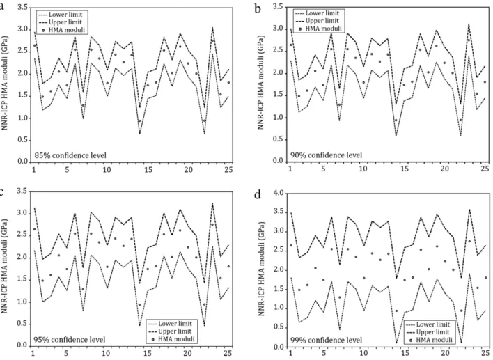
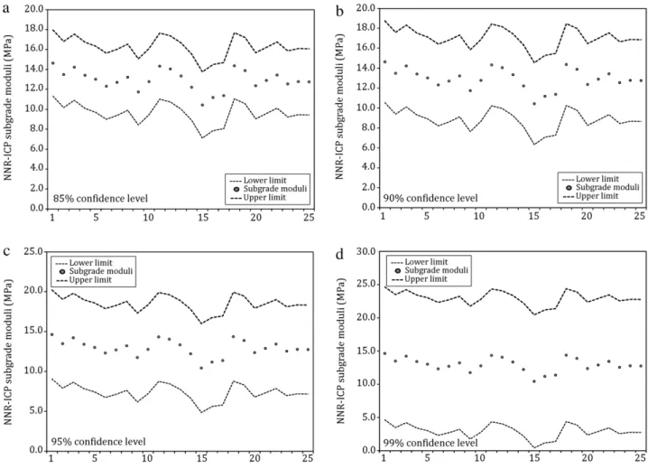
Figure 5displays the NNR-ICP prediction regions for HMA moduli at different confidence levels (or significance levels). Similar results are displayed for subgrade moduli inFigure 6. As the confidence level is upgraded, the corresponding prediction region is enlarged. Thus, the size of the prediction region depends on the pre-declared confidence level. Intuitively, higher confidence in the predictions implies larger prediction regions. Note that the same methodology can be applied to obtain pavement layer moduli prediction regions at pre-defined confidence levels from actual field NDT data, which could not be shown in this paper due to space limitations. For instance when backcalculation analysis based on field NDT data is carried out for pavement remaining life estimations, it would be beneficial to have a tolerance interval corresponding to the degree of uncertainty in such estimations. This information can
Figure 3: Calibration of NNR-ICP HMA moduli prediction model.
Figure 4: Calibration of NNR-ICP subgrade moduli prediction model.
be derived using the proposed NNR-ICP methodology, which is not possible with existing methodologies.
Among existing learning schemes that can be used for providing predictions coupled with confidence information, the Bayesian framework and the Probably Approximately Correct (PAC) theory are most prominent. However, these two approaches have severe limitations. For instance, Bayesian methods may be able to provide optimal decisions when one has a priori knowledge of the distribution that generates the data. For real-world problems, this knowledge is often unavailable and assumed arbitrarily. Therefore, the resulting confidence levels may not bound the percentage of expected errors, which signifies a major failure. Papadopoulos et al. [36] and Melluish et al. [37] demonstrated the misleading nature of Bayesian methods when their assumptions are violated.
Figure 5: Illustrative NNR-ICP HMA moduli prediction regions at different confidence levels.
The PAC theory has received considerable attention as it only assumes that the data arei.i.d.(independently and identically distributed) without knowing the exact distributions. Under a certain confidence level, the PAC theory can be used to produce an upper bound on the probability of error of an algorithm, which might be interesting in practice. However, the bounds obtained from these methods can be very loose and not very useful in practice if the data set is noisy. Additionally, the PAC theory has the following drawbacks:
1. It establishes bounds for the overall error and not for individual test examples.
2. Large explicit constants are involved in the majority of relevant results.
Other alternative ways of estimating machine learning algorithm prediction error rates include hold-out estimation, re-substitution, cross-validation, bootstrap, etc. In such cases, the training data set is used to derive the prediction rule (such as NN, SVM, etc.) that is applied to the test set, and the confidence of this prediction rule is simply based on the observed error rate on the test set. However, the reported confidence is strongly dependent on the chosen test data set and is not theoretically supposed to extrapolate to any new test example. In addition, these estimates assign a global error rate to all new examples without regard to their individualities [38].
A significant advantage of CP over the methods discussed above is that it provides valid and well-calibrated confidence measures that are useful in practice without assuming anything more thani.i.d.
4. Conclusions
Conformal Prediction (CP), also referred to as Confidence Machine, is a recently introduced promising framework that yields predictions coupled with confidence estimation. In re-cent years, several Artificial Intelligence (AI) based techniques have been proposed for the inverse analysis of pavement sys-tems and backcalculation of pavement moduli from pavement Non-Destructive Test (NDT) data. Especially, several research studies have focused on the development of Neural Networks Regression (NNR) based pavement inverse analysis models. But, so far, all AI methods developed for prediction of pavement layer moduli from NDT data yield only a ‘bare’ predictive value and do not report on the credibility and accuracy of the informa-tion. Without knowing the confidence of predictions, it is dif-ficult to measure and control the risk of error associated with the predictions. A valuable contribution of CP is that it can be coupled with most machine learning algorithms (like NN) to provide well-calibrated prediction regions rather than point predictions.
In this paper, an NNR-ICP approach is developed for making hedged predictions of pavement layer moduli with predefined confidence levels. In contrast to the original NN method, which outputs ‘bare’ predictions of pavement layer moduli, every prediction output by NNR-ICP is a set of possible values denoted as the ‘prediction region’ or ‘prediction interval’ (also known as the tolerance interval) from which the credibility and accuracy of pavement layer moduli predictions can be estimated. This information will be useful for the pavement engineer to assess
Figure 6: Illustrative NNR-ICP subgrade moduli prediction regions at different confidence levels.
the reliability of predictions at different pre-defined confidence levels. Going beyond the scope of the current study, the concept of CP has several useful applications in the context of mechanistic-empirical pavement design.
References
[1] Gopalakrishnan, K., Ceylan, H. and Attoh-Okine, N., Eds.,Intelligent and Soft Computing in Infrastructure Systems Engineering: Recent Advances, Springer, Inc., Germany (2010).
[2] Meier, R.W. and Rix, G.J. ‘‘Backcalculation of flexible pavement moduli from dynamic deflection basins using artificial neural network’’, Trans-portation Research Record, 1473, pp. 72–81 (1995).
[3] Ceylan, H., Guclu, A., Bayrak, M.B. and Gopalakrishnan, K. ‘‘Nondestructive evaluation of Iowa pavements-phase I’’, Final Report, CTRE, Iowa State University, Ames, IA, Iowa Department of Transportation (2007). [4] Bellotti, T., Luo, Z. and Gammerman, A. ‘‘Reliable classification of childhood
acute leukemia from gene expression data using confidence machines’’, IEEE International Conference on Granular Computing, Atlanta, USA (2006). [5] Gammerman, A., Vapnik, V. and Vovk, V. ‘‘Learning by transduction’’, InUncertainty in Artificial Intelligence, pp. 148–155, Morgan Kaufmann, London, UK (1998).
[6] Gammerman, A. and Vovk, V. ‘‘Prediction algorithms and confidence measures based on algorithmic randomness theory’’,Theoretical Computer Science, 287, pp. 209–217 (2002).
[7] Vovk, V. ‘‘On-line confidence machines are well-calibrated’’,43rd Annual Symposium on Foundations of Computer Science, pp. 187–196 (2002). [8] Vovk, V., Gammerman, A. and Shafer, G.,Algorithmic Learning in a Random
World, Springer, New York (2005).
[9] Gammerman, A. and Vovk, V. ‘‘Hedging predictions in machine learning’’, The Computer Journal, 50, pp. 151–177 (2007).
[10] Shafer, G. and Vovk, V. ‘‘A tutorial on conformal prediction’’,Journal of Machine Learning Research, 9, pp. 371–421 (2007).
[11] Dawid, A.P.,Probability forecasting, InEncyclopedia of Statistical Sciences, vol. 7, pp. 210–218, Wiley-Interscience, New York (1986).
[12] Saunders, C., Gammerman, A. and Vovk, V.,Transduction with confidence and credibility, In16th International Joint Conference on Artificial Intelligence, vol. 2, pp. 722–726, Morgan Kaufmann, Los Altos, CA (1999).
[13] Proedrou, K., Nouretdinov, I., Vovk, V. and Gammerman, A. ‘‘Transductive confidence machines for pattern recognition’’, In13th European Conference on Machine Learning, ECML’02, pp. 381–390, Springer, New York (2002). [14] Papadopoulos, H. ‘‘Inductive conformal prediction: theory and application
to neural networks’’, inTools in Artificial Intelligence, InTech., Vienna, Austria pp. 315–330 (Chapter 18). URL:http://www.intechopen.com/ download/pdf/pdfs_id/5294.
[15] Lambrou, A., Papadopoulos, H. and Gammerman, A. ‘‘Reliable confidence measures for medical diagnosis with evolutionary algorithms’’, IEEE Transactions on Information Technology in Biomedicine, 15(1), pp. 93–99 (2011).
[16] Nouretdinov, I., Melluish, T. and Vovk, V. ‘‘Ridge regression confidence machine’’,18th International Conference on Machine Learning, ICML’01, San Francisco, CA, pp. 385–392 (2001).
[17] Papadopoulos, H. and Haralambous, H. ‘‘Reliable prediction intervals with regression neural networks’’,Neural Networks, 24(8), pp. 842–851 (2011). [18] Gammerman, A., Vovk, V., Burford, B., Nouretdinov, I., Luo, Z., Chervo-nenkis, A., Waterfield, M., Cramer, R., Tempst, P., Villanueva, J., Kabir, M., Camuzeaux, S., Timms, J., Menon, U. and Jacobs, I. ‘‘Serum proteomic ab-normality predating screen detection of ovarian cancer’’,The Computer Journal, 52(3), pp. 326–333 (2008).
[19] Papadopoulos, H., Gammerman, A. and Vovk, V. ‘‘Reliable diagnosis of acute abdominal pain with conformal prediction’’,Engineering Intelligent Systems, 17(2–3), pp. 127–137 (2009).
[20] Lambrou, A., Papadopoulos, H., Kyriacou, E., Pattichis, C.S., Pattichis, M.S., Gammerman, A. and Nicolaides, A. ‘‘Assessment of stroke risk based on morphological ultrasound image analysis with conformal prediction’’, In6th IFIP International Conference on Artificial Intelligence Applications and Innovations, AIAI 2010, pp. 146–153, Springer, New York (2010). [21] Shahmuradov, I.A., Solovyev, V.V. and Gammerman, A. ‘‘Plant promoter
prediction with confidence estimation’’, Nucleic Acids Research, 33, pp. 1069–1076 (2005).
[22] Papadopoulos, H., Papatheocharous, E. and Andreou, A.S. ‘‘Reliable confidence intervals for software effort estimation’’,Workshops of the 5th IFIP Conference on Artificial Intelligence Applications & Innovations,
Thessaloniki, Greece, pp. 211–220 (2009). URL: http://ceur-ws.org/Vol-475/AISEW2009/22-pp-211-220-208.pdf.
[23] Saunders, C., Gammerman, A. and Vovk, V.,Computationally efficient transductive machines, InLecture Notes in Artificial Intelligence, vol. 1968, pp. 325–333, Springer, Berlin (2000).
[24] Papadopoulos, H., Proedrou, K., Vovk, V. and Gammerman, A.,Inductive confidence machines for regression, InLecture Notes in Computer Science, vol. 2430, pp. 334–356, Springer, Berlin (2002).
[25] Papadopoulos, H., Vovk, V. and Gammerman, A. ‘‘Qualified predictions for large data sets in the case of pattern recognition’’,2002 International Conference on Machine Learning and Applications, ICMLA’02, Las Vegas, Nevada, pp. 159–163 (2002).
[26] Brown, S.F. and Pappin, J.W. ‘‘Analysis of pavements with granular bases’’, Transportation Research Record, 810, pp. 17–23 (1981).
[27] Thompson, M.R. and Elliott, R.P. ‘‘ILLI-PAVE based response algorithms for design of conventional flexible pavements’’,Transportation Research Record, 1043, pp. 50–57 (1985).
[28] Adeli, H. ‘‘Neural networks in civil engineering: 1989–2000’’, Computer-Aided Civil and Infrastructure Engineering, 16, pp. 126–142 (2001). [29] Tsoukalas, L.H. and Uhrig, R.E.,Fuzzy and Neural Approaches in Engineering,
Wiley, New York (1997).
[30] Haykin, S.,Neural Networks: A Comprehensive Foundation, Prentice-Hall Inc., New Jersey (1999).
[31] Raad, L. and Figueroa, J.L. ‘‘Load response of transportation support systems’’,Journal of Transportation Engineering, ASCE, 106(1), pp. 111–128 (1980).
[32] Hicks, R.G. and Monismith, C.L. ‘‘Factors influencing the resilient properties of granular materials’’,Transportation Research Record, 345, pp. 15–31 (1971).
[33] Rada, G. and Witczak, M.W. ‘‘Comprehensive evaluation of laboratory resilient moduli results for granular material’’,Transportation Research Record, 810, pp. 23–33 (1981).
[34] Thompson, M.R. and Robnett, Q.L. ‘‘Resilient properties of subgrade soils’’, Journal of Transportation Engineering, ASCE, 105(1), pp. 71–89 (1979). [35] Gopalakrishnan, K., Ceylan, H. and Guclu, A. ‘‘Airfield pavement
deterio-ration assessment using stress-dependent neural network models’’, Struc-ture and InfrastrucStruc-ture Engineering, 5(6), pp. 487–496 (2009).
[36] Papadopoulos, H., Vovk, V. and Gammerman, A. ‘‘Regression conformal prediction with nearest neighbours’’, Journal of Artificial Intelligence Research, 40, pp. 815–840 (2011).
[37] Melluish, T., Saunders, C., Nouretdinov, I. and Vovk, V.,Comparing the Bayes and typicalness frameworks, InLecture Notes in Computersss Science, vol. 2167, pp. 360–371, Springer, Berlin (2001).
[38] Wang, H., Lin, C., Yang, F. and Hu, X. ‘‘Hedged predictions for traditional Chinese chronic gastritis diagnosis with confidence machine’’,Computers in Biology and Medicine, 39, pp. 425–432 (2009).
Kasthurirangan Gopalakrishnan is a Research Assistant Professor in the Department of Civil, Construction and Environmental Engineering at Iowa State University. He received his Ph.D. in Civil Engineering from the University of Illinois at Urbana-Champaign in 2004. His research interests include sustainable infrastructure, green engineering technology, bio-inspired computing, and smart pavements. Dr. Gopalakrishnan has published a textbook entitled, ‘‘Sustainable Highways, Pavements and Materials: An Introduction’’, and is also the lead editor of Springer’s ‘‘Sustainable and Resilient Critical Infrastructure Systems: Simulation, Modeling, and Intelligent Engineering’’, and ‘‘Soft Computing in Green and Renewable Energy Systems’’. He is also Associate Editor of theInternational Journal for Traffic and Transport Engineering.
Harris Papadopoulosreceived a B.S. (first Class Hons.) degree in Computer Science and a Ph.D. degree in Machine Learning from Royal Holloway, University of London, Surrey, UK, in 1999 and 2004, respectively. He is currently a Lecturer in the Department of Computer Science and Engineering of Frederick University, Nicosia, Cyprus, and a Visiting Fellow of the Computer Learning Research Centre of Royal Holloway, University of London, in the UK. He has published more than 30 research papers in international refereed journals and conferences, and has co-chaired two international conferences and workshops. His research interests include conformal prediction, computational learning, intelligent data analysis and the application of machine learning techniques to medical and engineering problems.