Working Paper Series
Estimation of linear dynamic
panel data models with
time-invariant regressors
Sebastian Kripfganz and Claudia Schwarz
Abstract
We propose a two-stage estimation procedure to identify the effects of time-invariant re-gressors in a dynamic version of the Hausman-Taylor model. We first estimate the coeffi-cients of the time-varying regressors and subsequently regress the first-stage residuals on the time-invariant regressors providing analytical standard error adjustments for the second-stage coefficients. The two-stage approach is more robust against misspecification than GMM esti-mators that obtain all parameter estimates simultaneously. In addition, it allows exploiting advantages of estimators relying on transformations to eliminate the unit-specific heterogene-ity. We analytically demonstrate under which conditions the one-stage and two-stage GMM estimators are equivalent. Monte Carlo results highlight the advantages of the two-stage ap-proach in finite samples. Finally, the apap-proach is illustrated with the estimation of a dynamic gravity equation for U.S. outward foreign direct investment.
Keywords: Dynamic panel data; Time-invariant variables; Two-stage estimation; System GMM; Dynamic gravity equation
Non-technical summary
Panel data comprises of cross-sectional units, e.g. countries, firms, households, or individuals, observed at different points in time. The combination of cross-sectional and time series data allows for richer econometric model specifications and more accurate conclusions. In addition, dynamic adjustment processes can be analyzed for a broad base of cross-sectional units. In a dynamic model past observations of the variable of interest can influence the current value. Macroeconomic output growth regressions and microeconomic wage regressions are examples where dynamic panel data models are used to account for the persistence of the dependent variable.
This paper analyzes the identification of effects of time-invariant regressors in dynamic panel data models as the methods currently used can be very imprecise or are not able to handle these regressors. Time-invariant regressors play an important role in many empirical applications but estimation of the effects is non-trivial because there are various statistical problems that may arise. We discuss the existing possibilities to estimate dynamic panel data models with time-invariant explanatory variables and we propose an alternative two-stage estimation procedure. A major advantage of the two-stage approach is that misspecified assumptions on the time-invariant regressors do not influence the estimation results for the coefficients of time-varying variables. In extensive simulation studies we show that the currently most widely used estimation method, the generalized method of moments, can be quite biased whereas our method provides more precise and robust results. Furthermore, we develop a correction term for the standard errors of the second stage. Neglecting the correction term can generate misleading implications.
To illustrate these methods we estimate a dynamic gravity model to explain real bilateral outward stocks of FDI for the United States. The data set was previously used by other authors to demonstrate instrumental variable methods for static panel models with time-invariant regressors. In this case, the time-invariant variable of interest is geographical distance. We highlight the relevance of a dynamic model specification, the benefits of the proposed two-stage approach, and the importance of adequately correcting the standard errors.
1
Introduction
This paper considers estimation methods and inference for linear dynamic panel data models with a short time dimension. In particular, we focus on the identification of coefficients of time-invariant variables in the presence of unobserved unit-specific effects. In many empirical applications time-invariant variables play an important role in structural equations. In labor economics researchers are interested in the effects of education, gender, nationality, ethnic and religious background, or other time-invariant characteristics on the evolution of wages but would still like to control for unobserved time-invariant individual-specific effects such as worker’s ability. As a recent example, Andini (2013) estimates a dynamic version of the Mincer equation controlling for a rich set of time-invariant characteristics. In macroeconomic cross-country studies institutional features or group-level effects play a role in explaining economic development. For example, Hoeffler (2002) studies the growth performance of Sub-Saharan Africa countries by introducing a regional dummy variable in her dynamic panel data model. Cinyabuguma and Putterman (2011) focus on within Sub-Saharan differences by adding socio-economic and geographic factors to the analysis. The analysis of bilateral trade or foreign direct investment (FDI) determinants is often based on gravity models with geographical distance as a key time-invariant factor. To account for the persistence of trade flows or FDI, Kimura and Todo (2010), Olivero and Yotov (2012), and Kahouli and Maktouf (2014) set up dynamic gravity equations.
If there is unobserved unit-specific heterogeneity, it is often hard to disentangle the effects of the observed and the unobserved time-invariant heterogeneity. Standard fixed and random effects estimators cannot be used because of multicollinearity problems and, when the time dimension is short, the familiar Nickell (1981) bias in dynamic panel data models. Therefore, it is common prac-tice in empirical work to apply the generalized method of moments (GMM) framework proposed by Arellano and Bond (1991), Arellano and Bover (1995), and Blundell and Bond (1998), amongst others. However, as Binder et al. (2005) and Bun and Windmeijer (2010) emphasize, GMM estima-tors might suffer from a weak instruments problem when the autoregressive parameter approaches unity or when the variance of the unobserved unit-specific effects is large. Moreover, the number of instruments can rapidly become large relative to the sample size. The consequences of instrument proliferation, summarized by Roodman (2009), range from biased coefficient and standard error
estimates to weakened specification tests.
In order to overcome the weak instruments problem in the context of estimating the effects of time-varying regressors, Hsiao et al. (2002) propose a transformed likelihood approach that is based on the model in first differences. A shortcoming of this approach is the inability to estimate the coefficients of time-invariant regressors. In this paper, we propose a two-stage estimation procedure to identify the latter. In the first stage, we estimate the coefficients of the time-varying regressors. Subsequently, we regress the first-stage residuals on the time-invariant regressors.1 We achieve identification by using instrumental variables in the spirit of Hausman and Taylor (1981), and adjust the second-stage standard errors to account for the first-stage estimation error. Our methodology applies to any first-stage estimator that consistently estimates the coefficients of the time-varying variables without relying on coefficient estimates for the time-invariant regressors. Among others, the quasi-maximum likelihood (QML) estimator of Hsiao et al. (2002) as well as GMM estimators qualify as potential first-stage candidates. A major advantage of the two-stage approach is the invariance of the first-stage estimates to misspecifications regarding the model assumptions on the correlation between the time-invariant regressors and the unobserved unit-specific effects.2 However, under particular conditions feasible efficient one-stage and two-stage GMM estimation are shown to be (asymptotically) equivalent.
We perform Monte Carlo experiments to evaluate the finite sample performance in terms of bias, root mean square error (RMSE), and size statistics of our two-stage procedure relative to GMM estimators that obtain all coefficient estimates simultaneously. The results suggest that the two-stage approach is to be preferred when the researcher is interested in the coefficients of both time-varying and time-invariant variables. However, the quality of the second-stage estimates de-pends crucially on the precision of the first-stage estimates. Among our first-stage candidates the QML estimator performs very well. GMM estimators can be an alternative if effective measures are taken to avoid instrument proliferation. Our Monte Carlo analysis unveils sizable finite sample 1For a static model, Pl¨umper and Troeger (2007) propose a similar three-stage approach that they label fixed effects vector decomposition. Their first stage is a classical fixed effects regression. In a recent symposium on this method, Breusch et al. (2011) and Greene (2011) show that the first two stages can be characterized by an instrumental variable estimation with a particular choice of instruments, and that the third stage is essentially meaningless.
2Hoeffler (2002) and Cinyabuguma and Putterman (2011) argue similarly. They apply GMM estimation in the first stage, and ordinary least squares estimation in the second stage. However, they do not correct the second-stage standard errors.
biases when the GMM instruments are based on the full set of available moment conditions, in particular regarding the coefficients of time-invariant regressors. Finally, in contrast to conven-tionally computed standard errors our adjusted second-stage standard errors account remarkably well for the first-stage estimation error.
To illustrate these methods we estimate a dynamic gravity equation for FDI based on U.S. data previously employed by Egger and Pfaffermayr (2004a). We find strong evidence for history dependence of the real bilateral stock of outward FDI. Neglecting the dynamic nature of the model results in a sizable overestimation of the effect of the time-invariant geographical distance variable. Again, the correct adjustment of the second-stage standard errors proves to be important for valid inference.
The paper is organized as follows: Section 2 introduces the dynamic Hausman and Taylor (1981) model. Section 3 describes one-stage GMM estimators that identify all coefficients simultaneously, while Section 4 lays out the two-stage procedure that yields sequential coefficient estimates. Section 5 contrasts the two approaches on theoretical grounds, while Section 7 provides simulation evidence on the performance of the two-stage approach in comparison to one-stage GMM estimators under different scenarios. In Section 8 we discuss the empirical application, and Section 9 concludes.
2
Model
Consider the dynamic panel data model with unitsi = 1,2, . . . , N, and a fixed number of time periodst= 1,2, . . . , T, withT ≥2:
yit=λyi,t−1+x0itβ+fi0γ+eit, eit=αi+uit, (1)
wherexit is aKx×1 vector of time-varying variables. The initial observations of the dependent
variable,yi0, and the regressors,xi0, are assumed to be observed. fi is aKf×1 vector of observed
time-invariant variables that includes an overall regression constant, andαiis an unobserved
unit-specific effect of thei-th cross section. In a strict sense,αiis called a fixed effect if it is allowed to be
correlated with all of the regressor variablesxitandfi, and it is a random effect if it is independently
paper we look at a hybrid (or intermediate case) of the dynamic fixed and random effects models where some of the regressors are correlated withαibut not all of them. Throughout the paper we
maintain the following assumptions:
Assumption 1: The disturbancesuitand the unobserved unit-specific effectsαiare independently
distributed acrossiand satisfyE[uit] =E[αi] = 0,E[uisuit] = 0∀s6=t, andE[αiuit] = 0.
Identification of the (structural) parametersλ,βandγnow crucially hinges on the assumptions about the dependencies between the regressors and the unit-specific effects.
Assumption 2: The explanatory variables can be decomposed as xit = (x01it,x02it)0 and fi =
(f10i,f20i)0 such thatE[αi|x1it,f1i] = 0,E[αi|x2it]6= 0 andE[αi|f2i]6= 0.
The resulting model is the dynamic counterpart of the Hausman and Taylor (1981) model. For further reference, the lengths of the subvectors areKx1, Kx2, Kf1, and Kf2, respectively. If
Kx2 =Kf2 = 0 the model collapses to the dynamic random effects model. Contrarily, Kx1 = 0 and Kf1 = 1 (the constant term) leads to the dynamic fixed effects model. In the remaining sections, we occasionally distinguish between strictly exogenous and predetermined regressorsxit
with respect to the disturbance termuit.
Assumption 3: The time-invariant regressors fi are exogenous with respect to the disturbances
uit, while the time-varying regressorsxitcan be strictly exogenous,E[uit|xi0,xi1, . . . ,xiT,fi;αi] =
0, or predetermined,E[uit|xi0,xi1, . . . ,xit,fi;αi] = 0 andE[uit|xis]6= 0∀s > t.3
To facilitate the subsequent derivations we introduce the following notation. We can write model (1) as
yi=λyi,(−1)+Xiβ+Fiγ+ei, ei =αiιT +ui, (2)
where yi = (yi1, yi2, . . . , yiT)0 is the vector of stacked observations of the dependent variable for
uniti. yi,(−1),Xi,Fi, ei, andui are defined accordingly. ιT is aT ×1 vector of ones. When the
3For simplicity, we abstract from endogenous regressors with respect tou
it. They can be easily incorporated by
data is stacked for all units, for exampley= (y01,y02, . . . ,y0N)0, subscripts are omitted:
y=λy(−1)+Xβ+Fγ+e, e=α+u. (3)
Finally, letW= (y(−1),X) be the matrix of time-varying regressors with corresponding coefficient vectorθ= (λ,β0)0, and ˜W= (y(−1),X,F) be the full regressor matrix.
3
One-Stage GMM Estimation
We can estimate all model parameters simultaneously by choosing appropriate instruments for the variables that are endogenous with respect to the unobserved unit-specific effects. In the following, we discuss generalized method of moments estimators that are based on the linear moment conditions
E[Z0iHei] =0, (4)
whereZi is a matrix ofKz instruments, andH is a deterministic transformation matrix.
For the static model with strictly exogenous regressorsxit, Hausman and Taylor (1981) propose
an instrumental variable estimator that uses deviations from their within-group means, xit−x¯i,
as instruments for the regressors xit, and the within-group means ¯x1i as instruments for f2i.4
The time-invariant regressorsf1i serve as their own instruments. We can extend this estimator to
the dynamic model by adding an appropriate instrument for the lagged dependent variable. For example, Anderson and Hsiao (1981) propose to useyi,t−2 or ∆yi,t−2 as instruments for ∆yi,t−1. Withyi,(−2) = (yi0, yi1, . . . , yi,T−2)0, the resulting estimator satisfies the moment conditions (4) with Zi= yi,(−2) 0 0 0 0 Xi 0 0 0 0 X1i F1i , and H= D Q P ,
for the (T−1)×T first-difference transformation matrixD= [(0,IT−1)−(IT−1,0)], whereIT−1 is the identity matrix of orderT−1, and theT×T idempotent and symmetric projection matrices 4To improve on the efficiency of the estimator, Amemiya and MaCurdy (1986) propose to use all time periods of
x1itseparately as instruments instead of the within-group means. Breusch et al. (1989) additionally suggest using
P = ιT(ι0TιT)−1ι0T and Q = IT −P, where P and Q transform the observations into
within-group means and deviations from within-within-group means, respectively. Importantly, bothD andQ are orthogonal to time-invariant variables. Due to the block-diagonal structure of Zi, only the
instruments (X1i,F1i) in the lower-right block of Zi are of use to identify γ. Therefore, as in
the static model of Hausman and Taylor (1981), a necessary condition for the identification of all coefficients (θ0,γ0)0 with this extended estimator isKx1≥Kf2.
Since the above estimator does not exploit all model implied moment conditions, it will be inefficient. Arellano and Bond (1991), Arellano and Bover (1995), and Blundell and Bond (1998) derive additional linear moment conditions for the model in first differences and in levels. Ahn and Schmidt (1995) add further moment conditions under homoscedasticity ofuitthat are in part
nonlinear. We present the full set of linear moment conditions in Appendix A. For the equations in first differences, E[Z0diDei] = 0, and in levels, E[Z0liei] = 0, the moment conditions can be
combined by defining Zi= Zdi 0 0 Zli , and H= D IT
in equation (4). It is well documented by Blundell and Bond (1998) and others (in the absence of time-invariant regressors) that the GMM estimator with instruments for the first-differenced equation only suffers from a potentially severe weak instruments problem whenλ→1. Under an additional mean stationarity assumption, Assumption 5 in Appendix A, they suggest to addition-ally use the first differences of the time-varying variables as instruments for the equation in levels. However, Bun and Windmeijer (2010) demonstrate that these instruments also can become weak, in particular when the variance ratio of the unit-specific effects relative to the idiosyncratic error term exceeds unity. To the contrary, the instruments for the first-differenced equation may regain strength when mean stationarity is not satisfied, as demonstrated by Hayakawa (2009).
Yet, sinceDιT =0, the instruments that are relevant for the identification of the coefficients
γ need to be placed inZli. Following Arellano and Bond (1991) and Arellano and Bover (1995),
2 for the model in levels: E[x1i0ei1] =0, and E[x1iteit] =0, t= 1,2, . . . , T, (5) E " T X t=1 f1ieit # =0. (6)
Consequently, in the absence of external instruments a necessary condition for the identification of all coefficients (θ0,γ0)0 in equation (1) is that Kx1(T + 1) ≥Kf2.5 Because levels instead of
first differences of the variablesx1it (andf1i) are used in the moment conditions (5) and (6), the
aforementioned weak instruments problem by Bun and Windmeijer (2010) is not an issue here. Nevertheless, a general weak correlation problem of the instruments x1it with the instrumented
regressorsf2i might still occur.
Remark 1: In practice, it will often be hard to justify that separate time periods of the ex-ogenous varying regressors provide sufficient explanatory power for the instrumented time-invariant regressors after partialling out the initial observations or within-group means, that is E[f2i|x1i0,X1i,f1i] =E[f2i|x1i0,f1i] orE[f2i|x1i0,X1i,f1i] =E[f2i|x¯1i,f1i]. The identification
con-dition then tightens again toKx1≥Kf2.
Define ˜H=IN ⊗H, where⊗denotes the Kronecker product. Based on the sample moments
N−1Z0He˜ , we can now derive the GMM estimator that minimizes the following distance function:
ˆ θ ˆ γ = arg minθ,γ e 0H˜0ZV NZ0He˜ ,
whereVN is a positive definite weighting matrix. If all elements in (θ0,γ0)0 are identified, that is
˜ W0H˜0ZVNZ0H˜W˜ is non-singular, we obtain ˆ θ ˆ γ = ˜ W0H˜0ZVNZ0H˜W˜ −1 ˜ W0H˜0ZVNZ0Hy˜ . (7)
The following familiar result under the data generating process (1) applies:6
Lemma 1: If the moment conditions (4) are satisfied and all coefficients are identified, then under standard regularity conditions the joint asymptotic distribution of the one-stage GMM estimator (7) is: √ N ˆ θ−θ ˆ γ−γ a ∼ N(0,Σ), (8) with Σ = (S0VS)−1S0VΞVS(S0VS)−1, (9)
whereS= plimN−1Z0H˜W˜ , Ξ = plimN−1Z0Hee˜ 0H˜0Z, andV= plimVN.
From equation (9) in Lemma 1 we can infer the following statement on the efficiency of the GMM estimator:7
Lemma 2: The GMM estimator is asymptotically efficient for a given instruments matrix Zand transformation matrix ˜HifV= Ξ−1.
Blundell and Bond (1998) and Windmeijer (2000) emphasize that for dynamic panel data models, in general, efficient GMM estimation is infeasible without having a prior estimate of Ξ. A feasible efficient GMM estimator can be obtained in two steps. In the first step, choosing any positive definite matrixVN will yield consistent but generally inefficient estimates ˆθ and ˆγ.
The second-step estimator is then based onVN = ˆΞ−1. A consistent unrestricted estimate of Ξ is
obtained as ˆΞ =N−1PN
i=1Z
0
iHˆeiˆe0iH0Zi, with ˆei=yi−Wiˆθ−Fiγˆ.8 The importance of choosing
an appropriate first-step weighting matrix should not be underestimated in applied work. Although the second-step GMM estimator is asymptotically unaffected, its finite sample performance still depends on the choice ofVN in the first step. Windmeijer (2005) shows that asymptotic standard
error estimates of the two-step GMM estimator can be severely downward biased in finite samples. He derives a finite sample variance correction. Alternatives to the two-step GMM estimator that
6See for instance Hansen (1982), Theorem 3.1, or Newey and McFadden (1994), Theorem 3.4.
7This result dates back to Hansen (1982), Theorem 3.2, and was generalized by Newey and McFadden (1994), Theorem 5.2.
are targeted to improve the finite sample performance include the iterated and the continuously updated GMM estimators, see for example Hansen et al. (1996).
Moreover, GMM estimators might suffer from severe finite sample distortions that arise from having too many instruments relative to the sample size, as stressed by Roodman (2009) among others. The instrument count can be reduced by forming linear combinationsZiRof the columns
ofZi. For any deterministic transformation matrixR, this also leads to a valid set of moment
con-ditions,E[R0Z0
iHei] =0. The GMM estimator (7) is then based on the transformed instruments
ZiR. We provide examples of relevant transformation matrices in Appendix C.
4
Two-Stage Estimation
When estimating all regression coefficients simultaneously, a misclassification of time-invariant regressors as being uncorrelated with the unit-specific effects might lead to a biased estimation of all coefficients includingλ and β. In this section, we lay down a robust two-stage estimation procedure. In a first stage, we subsume the time-invariant variablesfiunder the unit-specific effects,
˜
αi =αi+fi0γ, and consistently estimate the coefficientsλandβindependent of the assumptions
on the correlation structure betweenfi andαi. In the second stage, we recoverγ.
The first-stage model is
yit=λyi,t−1+x0itβ+ ¯α+ ˜eit, e˜it= ˜αi−α¯+uit, (10)
where ¯α=E[ ˜αi]. To obtain the first-stage estimates ˆλand ˆβwe can apply a transformation that
eliminates the time-invariant unit-specific effects ˜αi. In particular, the GMM estimator of Arellano
and Bond (1991) and the QML estimator of Hsiao et al. (2002) are based on the first-differenced model, while Arellano and Bover (1995) propose a GMM estimator based on forward orthogonal deviations. Alternatively, system GMM estimators as discussed in Section 3 that also make use of the level relationship can be applied taking into account that the time-invariant variables fi
are now part of the first-stage error term ˜eit. If Kx1 >0 but some or all of the variables in x1it
are correlated withfi then these variables are uncorrelated with αi but not with ˜αi. Hence, the
particular first-stage estimator but make the following assumption:9
Assumption 4: ˆθis a consistent asymptotically linear first-stage estimator with influence function
ψi such that √ N(ˆθ−θ) = √1 N N X i=1 ψi+op(1), (11) E[ψi] = 0, andE[ψiψ0i] = Σθ.
Asymptotic normality of ˆθ follows under standard regularity conditions.10 Also, denote ψ =
PN
i=1ψi.
In the second stage, we estimate the coefficientsγ of the time-invariant variables based on the level relationship:
yit−λyˆ i,t−1−x0itβˆ =fi0γ+vit, vit=αi+uit−(ˆλ−λ)yi,t−1−x0it( ˆβ−β). (12)
In particular, note the two additional terms in the error term vit that are due to the first-stage
estimation error such that this second-stage error term is no longer independent and identically distributed. We can now set up a second-stage GMM estimator based on the asymptotic moment conditions lim N→∞E " 1 N N X i=1 Z0γivi # =0. (13)
Under Assumption 2, we can use the observationsx1itas instruments for the endogenous regressors
f2i. The resulting non-redundant asymptotic moment conditions are similar to those given by
equations (5) and (6): lim N→∞E " 1 N N X i=1 x1i0vi1 # =0, and lim N→∞E " 1 N N X i=1 x1itvit # =0, t= 1,2, . . . , T, (14) lim N→∞E " 1 N N X i=1 T X t=1 f1ivit # =0. (15)
9We pick up the case of a first-stage GMM estimator in the next section. Two-stage QML estimation is briefly discussed in Appendix E.
The corresponding instruments matrix is given asZγi= (Zxi,F1i), with Zxi= x01i0 x01i1 0 · · · 0 0 0 x01i2 ... .. . ... . .. 0 0 0 · · · 0 x01iT ,
which is valid both for strictly exogenous and predetermined variablesx1it. Consequently, the order
condition from the previous section transmits to the second-stage GMM estimation: A necessary condition for the identification of the coefficientsγ in equation (12) is thatKx1(T + 1)≥Kf2.11
The second-stage GMM estimator then solves12
ˆ ˆ γ= arg min γ v 0Z γVγNZ0γv,
for a positive definite weighting matrixVγN. When γ is identified, the second-stage GMM
esti-mator is given by:
ˆ ˆ
γ= F0ZγVγNZ0γF
−1
F0ZγVγNZγ0(y−Wˆθ). (16)
We can now formulate the following proposition:
Proposition 1: If Assumption 4 holds, the moment conditions (4) are satisfied and all coefficients are identified, then under standard regularity conditions the asymptotic distribution of the second-stage GMM estimator (16) is:
√
Nγˆˆ −γ∼ Na (0,Σγ), (17)
with
Σγ = (S0FVγSF)−1SF0VγΞvVγSF(S0FVγSF)−1, (18)
whereSF = plimN−1Z0γF, Ξv = plimN−1Z0γvv0Zγ, andVγ = plimVγN. Moreover,
Ξv= Ξe+SWΣθS0W −Ξ0θeS0W−SWΞθe, (19)
11The qualifications of Remark 1 apply again.
whereSW = plimN−1Zγ0W, Ξe= plimN−1Z0γee0Zγ, and Ξθe= plimN−1ψe0Zγ.
Proof. Inserting model (3) into equation (16) and scaling by√N we obtain: √ Nγˆˆ −γ= 1 NF 0Z γ VγN 1 NZ 0 γF −11 NF 0Z γ VγN 1 √ NZ 0 γv = (S0FVγSF)−1SF0Vγ 1 √ NZ 0 γe−SW √ N(ˆθ−θ) +op(1) = (S0FVγSF)−1SF0Vγ " 1 √ N N X i=1 (Z0γiei−SWψi) # +op(1),
where the last equality follows from Assumption 4. By applying the central limit theorem, N−1/2PN
i=1(Z
0
γiei−SWψi) a
∼ N(0,Ξe+SWΣθSW0 −Ξ0θeS0W−SWΞθe), and equation (18) follows
from the continuous mapping theorem.13
Remark 2: For completeness, the asymptotic covariance matrix between the first-stage and the second-stage estimator is given by
lim N→∞E ˆ θ−θ γˆˆ−γ 0 = (ΣθS0W + Ξθe)VγSF(S0FVγSF)−1. (20)
In analogy to Lemma 2, we can state the following corollary:
Corollary 1: The second-stage GMM estimator ˆγˆ is efficient for a given first-stage estimator ˆθ
and instruments matrixZγ ifVγ = Ξ−v1.
Similar to one-stage GMM estimators, feasible efficient estimation requires an initial estimate of Ξv unlessZ0γFis non-singular. A consistent unrestricted estimate of Ξ is obtained as
ˆ ˆ Ξv=Ξˆˆe+SˆˆWΣˆθSˆˆ0W − ˆ ˆ Ξ0θe ˆ ˆ S0W− ˆ ˆ SWΞˆˆθe, (21)
whereSˆˆW =N−1Z0γW. An estimate of Σθ is readily available from the first-stage regression. An
estimate of Ξe can be obtained as Ξˆˆe = N−1P N i=1Z
0
γiˆˆeieˆˆ0iZγi, where ˆˆei =yi−Wiˆθ−Fiˆˆγ for
a consistent initial estimate ˆγˆ. Obtaining an estimate of Ξθe is more involved as it relies on the
product of the influence functionψi from the first stage and the moment function from the second stage:14 ˆ ˆ Ξθe= 1 N N X i=1 ˆ ψiˆˆe0iZγi. (22)
Importantly, ignoring the first-stage estimation error by settingΞˆˆv =Ξˆˆe might not only yield an
inefficient second-stage estimator but also produces inconsistent standard error estimates of ˆγˆ. In general, the direction of the bias of uncorrected standard errors is a priori unclear unless Ξθe=0.
In the latter case, the difference Ξv −Ξe = SWΣθS0W is a positive semi-definite matrix and,
consequently, standard error estimates ignoring the correction term will be too small.15 Ξ
θe=0
holds for example in the special case where we consider a first-stage GMM estimator that uses moment conditions for the first-differenced model only, that isH=D, all second-stage instruments Zγiare time-invariant, and the errorsuitare independent and homoscedastic across units and time.
Finally, ignoring the first stage is only valid ifSW =0.
Remark 3: As an alternative to the strong Assumption 2 that requires some regressors to be uncorrelated with the unobserved unit-specific effectsαiin model (1), we can consider a correlated
random effects assumption in the spirit of Mundlak (1978),E[αi|Xi,Fi] =b+ ¯x0iπ, or Chamberlain
(1982),E[αi|Xi,Fi] =b+P T s=0x
0
isπs. Notice that the time-invariant regressors are part of the
conditioning set but do not appear at the right-hand side. Either of these assumptions allows the time-varying regressors to be correlated with the unobserved effects, although not in an arbi-trary way. The time-invariant regressors are as well allowed to be correlated with them but only indirectly through their correlation with the within-group means ¯xi or some linear combination
of the observationsxis. Taking for example the Mundlak (1978) approach, we can then replace
αi =b+ ¯x0iπ+ηi in the second-stage equation (12) and treat ¯xi as additional time-invariant
re-gressors. In this situation, all time-invariant variables serve as instruments for themselves and the coefficientsγ can be consistently estimated at the second stage (besides the regression constant for which we obtain plim ˆγˆ1=γ1+b).
14We derive the influence function for a first-stage GMM estimator in Appendix D and for a first-stage QML estimator in Appendix E.
5
One-Stage versus Two-Stage GMM Estimation
We are now in a position to shed more light on one-stage and two-stage GMM estimators and to contrast the two. To facilitate the following exposition, denote by (ˆθ0s,γˆ0s)0 the one-stage system GMM estimator (7) and decompose its weighting matrixVN =LL0 with rk(L) =Kz. Also define
y∗ = L0Z0Hy˜ , W∗ = L0Z0HW˜ , and F∗ =L0Z0HF˜ . The following partitioned regression result will be helpful: ˆ θs= (W∗0MFW∗)−1W∗0MFy∗, (23) ˆ γs= (F∗0F∗)−1F∗0 y∗−W∗θˆ, (24) whereMF =IKz−F
∗(F∗0F∗)−1F∗0 is an idempotent and symmetric projection matrix.
Further-more, partition the weighting matrix as
VN = VdN VdlN VdlN0 VlN , (25)
conformable for multiplicationsZdVdNZ0d andZlVlNZ0l. As an alternative consider the two-stage
GMM estimator (ˆθ0d,γˆˆ0d)0, where ˆθd is based on the moment conditions E[Z0diDei] = 0for the
transformed model only, and with weighting matrixVθN:
ˆ θd = W0D˜0ZdVθNZ0dDW˜ −1 W0D˜0ZdVθNZ0dDy˜ , (26)
where ˜D=IN ⊗D. The second-stage estimator ˆˆγd is given by equation (16) based on ˆθd in the
first stage. We can now make the following claim:
Proposition 2: It holds that ˆθs= ˆθd, with ˆθs and ˆθd given by equations (23) and (26),
respec-tively, ifZ0lFis non-singular andVθN =VdN−VdlNVlN−1V
0
dlN.
Proof. Observe that F0H˜0Z= (F0D˜0Z
d,F0Zl) = (0,F0Zl) since ˜DF=0. Consequently,F∗0F∗ =
F0ZlVlNZ0lF. With Z
0
lF being non-singular, it follows that (F
∗0F∗)−1 = (Z0 lF) −1V−1 lN(F 0Z l)−1.
LetVθN =VdN−VdlNV−lN1V0dlN. Then, LMFL0=VN −VN 0 0 0 V−lN1 VN = VθN 0 0 0 ,
such that after straightforward algebra equation (23) boils down to equation (26). Alternatively, ifZ0dD˜0Wis non-singular as well, ˆθs= ˆθd= (Z0dD˜
0W)−1Z0
dD˜
0yindependent of the choice of the
weighting matrices.
WhenZ0lFis non-singular, the coefficientsγ are exactly identified because the time-invariant regressors are orthogonal to the instruments for the first-differenced equation. But then the in-struments for the level equation cannot be used any more to identify the coefficientsθ, and ˆθs
consequently equals ˆθd with an appropriate choice of the weighting matrix. A similar proposition
holds for the coefficientsγ under the additional restriction that the level instruments of the one-stage system GMM estimator equal the instruments of the second-one-stage GMM estimator,Zl=Zγ:
Proposition 3: With Zl = Zγ, it holds that ˆγs = ˆγˆd, with ˆγs and ˆˆγd given by equations (24)
and (16), respectively, ifZ0γFis non-singular,VθN =VdN, andVdlN =0.
Proof. WithF∗0F∗=F0ZlVlNZ0lFandZl=Zγ, equation (24) can be written as
ˆ γs= (F0ZγVlNZ0γF)− 1 F0ZγVlN(VlN−1V 0 dlNZ0dD˜ +Zγ0)(y−Wθˆs).
WithZ0γFbeing non-singular, this equation reduces further to
ˆ
γs= (Z0γF)−1(V−lN1VdlN0 Z0dD˜ +Zγ0)(y−Wθˆs).
Also, equation (16) becomes ˆγˆd = (Z0γF)−1Z0
γ(y−Wˆθd) independent of VγN. Consequently,
ˆ
γs = ˆˆγd if VdlN = 0 and ˆθs = ˆθd. The latter results as a consequence of Proposition 2 by
setting VθN =VdN−VdlNVlN−1V0dlN =VdN. Alternatively, ifZ0dD˜0W is non-singular as well,
Z0dD˜(y−Wθˆd) =0and again ˆθs= ˆθd without any restriction on the weighting matrices.
are equivalent for a particular choice of the weighting matrices if both utilize the same linearly independent instruments for the equation in levels and their number equals the count of time-invariant regressors. In this case, the first-stage GMM estimator of the two-stage approach is based on the moment conditions for the transformed model only. Leaving aside the trivial case of exact identification of the coefficients θ as well, we can now infer a statement on asymptotic efficiency. WhenVN is the optimal weighting matrix for the estimator ˆθsaccording to Lemma 2,
then an optimal weighting matrix for the estimator ˆθd is given by VθN =VdN−VdlNV−lN1V0dlN
as can be easily seen by calculating the partitioned inverse of VN. This corresponds to the
condition that is required by Proposition 2. However, for equivalence of the one-stage and the two-stage estimators, Proposition 3 requires a block-diagonal weighting matrix VN of the
one-stage estimator such thatVdlN =0. It is clear that this restricted estimator is less efficient than
the feasible efficient one-stage GMM estimator in general unless the optimal one-stage weighting matrix is indeed block-diagonal asymptotically. A relevant case where this holds is a restricted covariance structure of the error term,E[eie0i|Zi] =σα2ιTι0T+σ
2
uIT, together with time-invariance
of the level instruments Zli. In this case, the feasible efficient one-stage and two-stage GMM
estimators will be (asymptotically) identical, and therefore also have the same variance.
Remark 4: If the optimal weighting matricesVN orVθN are based on separate initial consistent
estimates (of σu2), the equivalence of VθN and VdN−VdlNV−lN1VdlN0 only holds asymptotically,
and the resulting feasible efficient estimators can be numerically different in finite samples, even if all other conditions of Propositions 2 and 3 are satisfied.
If the moment conditions for the level equation outnumber the time-invariant regressors, the one-stage and the two-stage GMM estimators will generally be different because the information contained in the level instrumentsZli is no longer exclusively used to identifyγ. A clear ranking
of the two estimators in terms of efficiency is not possible anymore. Also, a misspecification of the level moment conditions might now turn the coefficient estimates for the time-varying regressors inconsistent.
6
Testing the Overidentifying Restrictions
For the identification of the coefficients of the time-invariant regressors, Assumption 2 is crucial, and a testing procedure for the validity of the regressor classification is desirable. Whenever the model parameters are overidentified, we can proceed along the lines of the Hansen (1982) test. If we cannot reject the null hypothesis of joint validity of the overidentifying restrictions for the one-stage GMM estimator (7), this suggests that the model is correctly specified. A rejection of the test, however, is not very informative about the source of misspecification due to the typically large number of overidentifying restrictions. Besides a wrong classification of regressors as being uncorrelated with the unit-specific effects under the Hausman and Taylor (1981) Assumption 2, other reasons might be undetected serial correlation of the errors,16 a misclassification of predetermined (or endogenous) time-varying regressors as strictly exogenous, or a violation of the mean stationarity Assumption 5.
With regard to the moment conditions (5) and (6) that are of particular interest, a difference-in-Hansen test for a subset of the moment conditions as proposed by Eichenbaum et al. (1988) is not helpful either. The coefficientsγwill be generally unidentified under the restricted estimator that excludes the suspicious instruments, unless the instruments obtained from these moment conditions outnumbers the time-invariant regressors by more than the number of excluded instruments. Even if a difference-in-Hansen test is feasible, we might be confronted with a weak instruments problem under the restricted estimation if we exclude particularly relevant instruments.
The two-stage approach outlined in Section 4 offers a successive testing strategy. At the first stage, specification tests should be carried out to gain confidence in the consistency of the coeffi-cient estimates for the time-varying regressors. Subsequently, such model misspecifications can be excluded under the alternative hypothesis for the Hansen (1982) at the second stage. Based on the two-stage residuals ˆˆe,17 we can then compute the Hansen (1982) test statistic for the validity of the second-stage overidentifying restrictions only:
ˆ ˆ τγ = 1 √ N ˆ ˆ e0Zγ ˆ ˆ Ξ−v1 1 √ NZ 0 γˆˆe . (27)
16Arellano and Bond (1991) propose a test for serial correlation based on the first-differenced residuals.
17Notice that ˆˆe= ˆˆvbecause the first-stage estimation error drops out when inserting estimates for the unknown population parameters.
With an optimal weighting matrix Ξˆˆ−1
v , the test statistic has a limiting χ2 distribution with
Kzγ−Kf degrees of freedom, whereKzγ denotes the number of linearly independent second-stage
instruments inZγ. Importantly,Ξˆˆv is a consistent estimate of the variance matrix Ξv in equation
(19) that accounts for the first-stage estimation error.
7
Monte Carlo Simulation
7.1
Simulation Design
We conduct Monte Carlo experiments to analyze the finite sample performance of the two-stage approach in comparison to one-stage GMM estimators. To keep the simulations economical we consider a dynamic panel data model with a single time-varying regressor xit that is correlated
with the unobserved unit-specific effects, and one time-invariant regressorfi that is uncorrelated
with them. In practice, the researcher will typically face a larger number of regressors. While the fundamental results should carry over to larger-dimensional models, we note that finite sample dis-tortions of GMM estimators that result from too many overidentifying restrictions might aggravate by adding additional regressors. We generateyitand xit according to the following processes:
yit=λyi,t−1+βxit+γfi+αi+uit, uit iid ∼ N(0, σ2u), (28) and xit=φxi,t−1+νρfi+ν p 1−ρ2η i+it, it iid ∼ N(0, σ2), (29)
such thatxit is strictly exogenous with respect touit.18
The observed time-invariant variablefi is obtained as an independent binary variable from a
Bernoulli distribution with success probability p. The unobserved unit-specific effects αi and ηi
18Modelingx
itas predetermined or endogenous does not affect the qualitative conclusions regarding the coefficient
of the time-invariant regressor for appropriately adjusted GMM estimators. It will, however, turn the two-stage QML estimator inconsistent because the first-difference transformation at the first stage requires strict exogeneity.
are generated from a joint normal distribution: αi ηi ∼ N µα µη , σ2 α σαη σαη p(1−p) , (30)
such that the variances ofηiandficoincide. The particular design of the process forxitguarantees
that the correlation betweenxitandfican be altered while keeping the variance ofxitunchanged,
because V ar(xit) = 1 (1−φ)2 ν2p(1−p) +1−φ 1 +φσ 2 (31)
is independent ofρ. ν≥0 is introduced as a scale parameter. The correlation betweenxit andfi
is characterized by: Corr(xit, fi) =ρ s ν2p(1−p) ν2p(1−p) +1−φ 1+φσ 2 . (32)
Sinceρ∈[−1,1], it can be interpreted as a correlation coefficient net of the variation coming from it.
We set the long-run coefficientβ/(1−λ) = 1 and initialize the processes att=−50 with their long-run means given the realizations of the unit-specific effects:
yi,−50=xi,−50+ 1 1−λ(γfi+αi), (33) xi,−50= ν 1−φ ρfi+ p 1−ρ2η i , (34)
and discard the first 50 observations for the estimation. The covariance between the two unobserved fixed effectsαi andηi is set toσαη=σα
p
p(1−p)/2 which creates a positive correlation between xit and αi. We also fix γ = 1, σ2u = 1, ν = 1, p = 0.5 and µα = µη = 0. To ensure an
adequate degree of fit, we obtain the population value of the coefficient of determination for the first-differenced model, R2
∆y, in a similar fashion as Hsiao et al. (2002). For the data generating
process stated above it is given by
R2∆y= β 2σ2 β2σ2 + (1 +φ)(1−λφ)σu2 . (35)
We fixR2
∆y= 0.2 and determine σ2endogenously as
σ2 = R 2 ∆y 1−R2 ∆y (1 +φ)(1−λφ) β2 σ 2 u. (36)
Finally, we simulate the data with different combinations for the remaining parameters, namelyλ∈ {0.4,0.8,0.99},σ2α∈ {1,3},φ∈ {0.4,0.8}, andρ∈ {0,0.4}. The sample size under consideration
isT ∈ {4,9}andN ∈ {50,500}. In total, we do 3000 repetitions for each simulation.
For the two-stage approach we consider system GMM estimators and the QML estimator of Hsiao et al. (2002) as first-stage estimators. The latter is briefly described in Appendix E. We compare the two-stage QML estimator, “2s-QML”, to various GMM estimators that use different sets of instruments and recover the coefficient of the time-invariant regressor either in one or in two stages. First, we set up a system GMM estimator that exploits the full set of moment conditions given in Appendix A and recovers all parameters jointly in one stage, “1s-sGMM (full)”.19 Besides the moment conditions (40) and (44) that result from the presence of the time-invariant regressor, this estimator equals the one proposed by Blundell et al. (2000). To deal with the problems resulting from too many instruments, we set up an alternative system GMM estimator with a collapsed set of instruments, “1s-sGMM (collapsed)”.20 This reduces the number of instruments from 33 to 15 whenT = 4 and from 143 to 30 whenT = 9. Furthermore, we consider two-stage variants of both GMM estimators, “2s-sGMM (full)” and “2s-sGMM (collapsed)”, respectively. To compute the standard errors of the (first-stage) GMM estimators, we use the robust variance-covariance formula (9) with an unrestricted estimate of Ξ. All GMM estimators are feasible efficient estimators with an initial weighting matrix as chosen by Blundell et al. (2000). We apply the Windmeijer (2005) correction for the standard errors. The second-stage estimates are independent of the choice of the weighting matrix becauseγ is exactly identified. The corresponding standard errors are based on formula (18) taking into account the first-stage estimation error.
19We disregard the moment conditions (41) that are due to homoscedasticity. For the regression constant we exploit only the moment conditions (44) but not the conditions (40).
7.2
Simulation Results
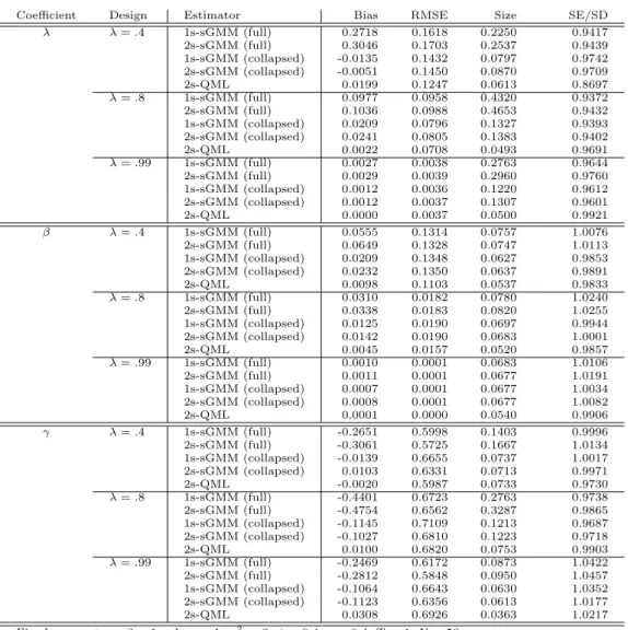
Table 1 summarizes the simulation results for different values of the autoregressive parameter λ holding fixedσ2α= 3,φ= 0.4, andρ= 0.4. The sample size is small withT = 4 andN = 50. As
a first observation, we recognize that the two-stage approach is very competitive. In particular for the coefficient of the time-invariant regressor it shows a smaller RMSE than the respective one-stage counterpart. We clearly see that the quality of the second-one-stage estimates hinges crucially on the choice of the first-stage estimator. The large bias of the GMM estimators with the full set of instruments readily transmits into poor second-stage estimates while the two-stage QML estimator convinces us with small biases irrespective of the parameter design.
[Table 1 about here.]
The finite sample bias of GMM estimators that exploit the full set of moment conditions can become tremendous. In the baseline scenario,λ= 0.4, it reaches 27 percent for the coefficient λ in case of one-stage estimation, and 30 percent for two-stage estimation. The magnitude is similar for the coefficientγ. Reducing the number of instruments with the collapsing procedure yields a strong bias reduction. It shrinks below 3 percent for all coefficients, comparable to the bias of the two-stage QML estimator. The root mean square error (RMSE) shows less clear a picture. While collapsing helps for the coefficient λ, it does not improve the RMSE for β and γ. Particularly for the latter, the reduced bias seems to come at the cost of a larger dispersion. Noteworthy, the RMSE of the two-stage estimator with the full set of instruments is lowest among all estimators under consideration for the coefficient of the time-invariant regressor. However, having a look at the size distortions it is clearly visible that this smaller RMSE does not compensate the poor performance in terms of bias relative to the GMM estimators with the collapsed instruments or the two-stage QML estimator.21
The average ratio of the estimated standard errors to the observed standard deviation of the estimators is in most cases reasonably close to unity. An exception are the QML estimates for the coefficientλwhen its true value is 0.4. Here, the standard error estimates fall short of the observed standard deviation by about 13 percent. This anomaly can be explained by the observation that 21Large size distortions of the Wald test for the system GMM estimator are also documented by Bun and Wind-meijer (2010) for the autoregressive parameter.
the QML estimates forλfeature a bimodal distribution with one peak close to the true value of 0.4 and another one close to unity.22 When we neglect those 44 estimates (out of 3000) that are larger than 0.8, the ratio of the standard errors to the standard deviation jumps up to 1.03. The problematic estimates of the first-stage QML estimator also affect the second-stage estimation of the coefficientγ. When the QML estimates ofλare above 0.8, then the majority of the second-stage estimates ofγ even has the wrong sign by falling below zero with a mean at −0.27. Irrespective of this effect, we obtain very promising results for the second-stage standard errors that correct for the first-stage estimation error. On average they are reasonably close to the observed standard deviation.
Increasing the persistence of the data generating process for yit does not produce a clear-cut
picture. For the coefficients of the time-varying regressors we obtain strong reductions both of the bias and the RMSE.23To the contrary, the GMM results deteriorate for the coefficient of the time-invariant regressor when changingλfrom 0.4 to 0.8 and improve again when increasingλto 0.99. We observe a similar non-uniform behavior for the size statistics with increasing values ofλ. The size distortions of the Wald tests for the GMM estimators first become larger when increasing λfrom 0.4 to 0.8 but become smaller again when heighteningλfurther to 0.99. In particular for the GMM estimators with the full set of instruments we notice large overrejections as a consequence of the considerable biases. For the two-stage QML estimator, the bias and RMSE get only slightly worse with higher persistence of the dependent variable.
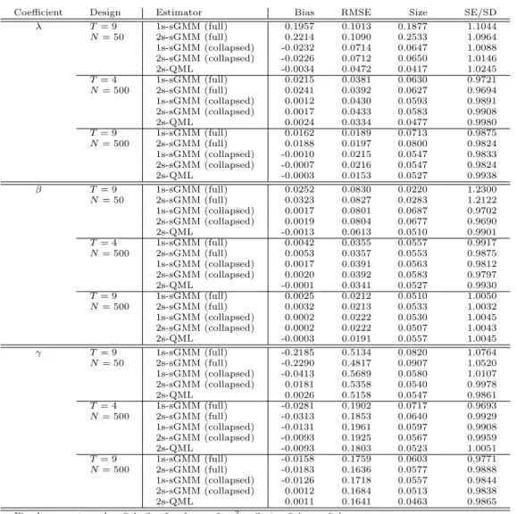
In Table 2 we present the simulation results for alternative sample sizes and with the same parameterization as in Table 1, holding fixedλ= 0.4. The findings are not surprising but a few observations shall be mentioned. For the GMM estimator with the full set of instruments both the bias and the RMSE are reduced when we increase the time dimension from 4 to 9 periods, despite the fact that the instruments count goes up from 33 to 143. When the cross-sectional dimension becomes large,N = 500, the RMSE turns in favor of the full set of instruments compared to the collapsed one while the latter is still preferred in terms of bias. Independent of the sample size, we find again that the two-stage GMM estimator shows a smaller RMSE than the corresponding one-stage estimator for the coefficient of the time-invariant regressor. For the QML estimator we 22Juodis (2013) provides a technical explanation for this identification problem of the transformed likelihood estimator in small samples.
can observe that the bimodal feature of the distribution disappears with increasingT orN.
[Table 2 about here.]
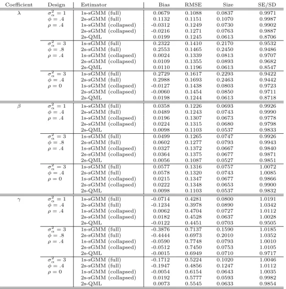
We also analyze the performance of the estimators under alternative parameterizations of the data generating process. Table 3 presents the results for the three situations of a reduction of the varianceσα2 of the unit-specific effects from 3 to 1, an increase in the persistence parameterφfrom
0.4 to 0.8, or an elimination of the correlation betweenxitandfiby settingρ= 0, respectively. In
the first case, the RMSE is reduced for all parameters. For the coefficient of the lagged dependent variable, the GMM estimators now even become superior to the QML estimator. This result is consistent with previous findings of Binder et al. (2005) and Bun and Windmeijer (2010) that GMM estimators tend to suffer from weak instruments when the variance of the unit-specific effects is large. In the second scenario, the higher persistence of xit yields small improvements for the
coefficients of the time-varying regressors. At the same time we observe a sharp deterioration of the results for the coefficient of the time-invariant regressor. The reason is that the latter now explains relatively less of the variation inyitdue to the larger variance of the regressorxit. Finally, removing
the correlation between the time-varying and the time-invariant regressor leaves the estimates for λandβ virtually unaffected but has a notably positive effect on the precision of the coefficient γ. Concerning the comparison of one-stage and two-stage estimators, the results in Table 3 largely confirm the picture of Table 1. The RMSE of the two-stage estimator is always smaller than that of the corresponding one-stage estimator for the coefficient of the time-invariant regressor while it is the other way round for the coefficients of the time-varying regressors.
[Table 3 about here.]
Importantly, irrespective of the simulation design, when we ignore the first-stage estimation error by assuming Ξv = Ξe in equation (18), we substantially underestimate the second-stage
standard errors. We contrast these estimates in Table 4. For the small sample size withT = 4 and N = 50 the uncorrected standard errors are on average 10 to 32 percent below the actual standard deviation of the coefficient estimates. Not surprisingly, the underestimation is less severe in the last simulation design where the exogenous time-varying and the time-invariant regressor are uncorrelated because this removes asymptotically the influence of the first-stage estimation
error in the coefficientβ on the second-stage estimates. A second noteworthy observation is that the standard error correction becomes less relevant when the sample size increases, in particular in the direction of observing more time periods.
[Table 4 about here.]
8
Empirical Application: Distance and FDI
Transportation costs play an important role in theoretical models of bilateral trade and direct investment determination. Empirically, geographical distance has been used extensively as a proxy for transportation costs in confronting gravity models with the data.24 A major complication in the estimation of such gravity equations with panel data is the time-invariant nature of the geo-graphical distance variable when controlling for unobserved country-specific, industry-specific, or firm-specific effects. While methods for fixed-effects models wipe out all time-invariant character-istics, a pure random-effects model may impose exogeneity assumptions that are too strong to be justifiable. A compromise between the two extremes is the Hausman and Taylor (1981) classifica-tion of regressors into subgroups of variables that are correlated with the unobserved effects and those that are not.
Egger and Pfaffermayr (2004a) extend this approach to a seemingly unrelated regressions (SUR) setup to identify the effects of distance on trade and FDI. The authors estimate a static SUR model based on bilateral data at the industry level for the United States and Germany, respec-tively.25 They argue that the geographic distance between two countries is correlated with the unobserved time-invariant propensity to invest abroad, for example due to decreasing cultural proximity. Therefore, appropriate instruments need to be deployed. The sum of the real gross domestic product of both countries (henceforth referred to as bilateral GDP), which is used as a predictor of outward FDI, is assumed to be correlated with unobserved trade-partner effects. A measure for the similarity in the country size as well as the factor endowments in physical and human capital are classified as truly exogenous in the sense of Assumption 2 and could thus serve
24See Egger and Pfaffermayr (2004a) and the references therein.
25The data set is available in the Journal of Applied Econometrics Data Archive. For a variable description, see Egger and Pfaffermayr (2004a). The data is observed on an annual basis for 341 bilateral industry-level relationships between 1989 to 1999. The panel is unbalanced with irregular patterns of missing observations.
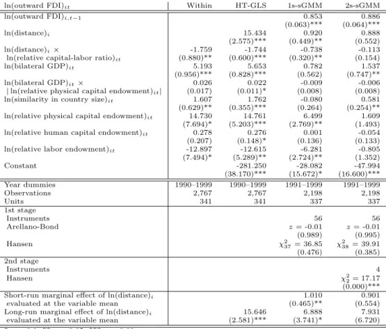
as instruments, while that is not the case for relative labor endowment in the FDI equation.26 While the SUR approach yields potential efficiency gains, estimating the model equation by equation still results in consistent estimates. We focus here on a re-estimation of the FDI model for the Unites States. In this case, Egger and Pfaffermayr (2004a) find a very large and statistically significant effect of distance, while for Germany and in the bilateral exports model the effect is either relatively small or even statistically insignificant. To assess the robustness of their results, we run a simple specification test for the static model. If there is no serial correlation in the idiosyncratic error term, the errors from the first-differenced equation should exhibit a serial correlation of -0.5.27 With the data at hand, it is estimated to be -0.113 which is significantly different from -0.5 at the 1% level. This result has several implications. First, standard errors should be made robust to serial correlation in a static fixed-effects regression for valid inference. Second, the generalized least squares (GLS) procedure used by Egger and Pfaffermayr (2004a) to obtain their Hausman and Taylor (1981) estimates is based on an incorrect estimate of the variance matrix. Third and most severe, if the serial correlation is a result of a data generating process that includes a lagged dependent variable, static model estimates potentially yield estimates with sizable biases of short-run and long-short-run effects as shown by Egger and Pfaffermayr (2004b).28 Given these arguments, we re-estimate the FDI equation for the United States in a dynamic setting.
The static model estimates based on the within transformation that removes all time-invariant components are replicated in the first column of Table 5. The coefficient estimates are identical to those in the original paper. Yet, we compute standard errors that are robust to heteroscedasticity and serial correlation. They are much higher compared to the conventional standard errors reported by Egger and Pfaffermayr (2004a) such that some of the regressors turn statistically insignificant or significant only at a lower level. The second column is a re-estimation of their single-equation GLS estimates under the Hausman and Taylor (1981) assumptions. Our coefficient estimates differ slightly from the original ones due to differences in the variance component estimates. However, 26In the bilateral exports equation, they still treat labor endowments as exogenous based on overidentification tests. However, to the extent that the unobserved time-invariant effects capture similar country-industry characteristics in both equations such an asymmetric treatment is disputable.
27See Wooldridge (2002, Chapter 10.6.3) for a description of the test.
28Besides this econometric argumentation in favor of a dynamic model specification, the recent literature on FDI determinants also motivates dynamic gravity models to cope with the persistence of bilateral FDI. See for example Kimura and Todo (2010) and Kahouli and Maktouf (2014). Both also employ system GMM estimators but remain silent on the instruments used to identify the coefficients of the time-invariant regressors.
the qualitative conclusions are the same.
[Table 5 about here.]
The dynamic model specification estimated with a system GMM estimator supports the as-sumption of history dependence in the data generating process of the real bilateral stock of outward FDI. The autoregressive coefficient exceeds 0.8 both with a one-stage and a two-stage estimation strategy.29 For the two-stage estimator, only 3 out of 56 instruments at the first stage differ from the one-stage estimator. More specifically, we are using first differences instead of levels of the variables that are assumed to be uncorrelated with the unobserved effects according to Assump-tion 2 (similarity in country size, relative physical capital endowment, and relative human capital endowment) as instruments for the equation in levels because they are partially correlated with the omitted distance variable. For our main variable of interest, the time-invariant geographical distance, the point estimates in both cases are very similar while the standard errors under the two-stage approach are much higher such that the coefficient estimate is no longer statistically significant.
When testing the validity of the dynamic model and instruments used, we find that the Hansen (1982) overidentification test based on the one-stage estimates does not provide evidence for mis-classification. We cannot reject the null hypothesis of joint validity of all instruments. The same holds for the first-stage estimation of our two-stage estimator. Contrarily, the test based on the second-stage estimates only rejects the chosen Hausman and Taylor (1981) classification of the variables.30 The Arellano and Bond (1991) specification test for absence of second-order serial correlation in the first-differenced residuals is easily passed by both estimators.
To address the potential invalidity of the second-stage instruments, we redo the analysis without 29The one-stage moment conditions are given in Appendix A, disregarding conditions (40) and (41). To avoid problems of instrument proliferation we only use the second to fourth lag of the dependent variable as instruments in the first-differenced equation and the lags 0 to 4 for the remaining regressors that are assumed to be strictly exogenous with respect to the idiosyncratic disturbances. In addition, we collapse the instrument matrices in accordance with the procedure described in Appendix C. We follow Blundell et al. (2000) to form the initial weighting matrix. For two-stage GMM estimation we treat all time-varying regressors as potentially correlated with the first-stage effects ˜
αi, as explained in Section 4. The second-stage moment conditions are given by equation (14), again applying
the collapsing procedure. At the second stage, we only report results from a one-step estimator without optimal weighting matrix because the feasible efficient estimator tends to be relatively sensitive when some of the instruments are weak.
30For its validity, the Hansen (1982) test statistic needs to be based on an optimal weighting matrix. Since we observed sensitive second-stage coefficient estimates when using an optimal weighting matrix in the presence of weak instruments, this may also undermine the reliability of the Hansen (1982) test. In the current case, the physical capital endowment is such an instrument that is only weakly correlated with distance.
classifying the relative physical capital endowment as an exogenous regressor with respect to the unobserved effects. Its unconditional correlation with the time-invariant distance variable is only 0.01. It is thus of no use to identify the coefficient of the latter. The results are reported in Table 6. We only observe minor changes in the coefficient estimates but the Hansen (1982) test no longer rejects the null hypothesis of joint validity of the remaining instruments (similarity in country size and relative labor endowment, in addition to a constant). Notice in particular that the estimates for the time-varying regressors with the two-stage estimator are entirely unaffected because the first-stage moment conditions remain the same as before.
[Table 6 about here.]
The estimation results hint at the appropriateness of a dynamic instead of a static model. For making the dynamic estimation results comparable with the static estimates, we compute the long-run marginal effect of distance evaluated at the mean of the relative capital-labor ratio (-0.12 in logarithms). In the dynamic model, the short-run effects are given by the marginal effects conditional on the lagged dependent variable while long-run effects are obtained by scaling the short-run effects by the multiplier (1−λ)−1. Both in Table 5 and 6 we can see that the implied long-run effect of distance on the real bilateral stock of outward FDI is much smaller in the dynamic model (and insignificant when using the two-stage estimator).
Finally, the correction of the second-stage standard errors as emphasized in Section 4 proves to be important. Table 6 reports the uncorrected standard errors in the final column. For the time-invariant distance variable, it is more than halved without the correction which would signal erroneously statistical significance even at the 1% level. Similar observations can be made for the short-run and long-run marginal effects. At the same time, the Hansen (1982) test would reject the null hypothesis of joint validity of the second-stage instruments at the 10% level if it is based on an uncorrected and therefore no longer optimal weighting matrix.
Overall, the static model estimates by Egger and Pfaffermayr (2004a) tend to strongly over-estimate the effect of distance on bilateral FDI due to the ignored persistence of the dependent variable. Moreover, the results from the dynamic model obtained with system GMM estimators remain inconclusive whether the effect is even statistically significantly different from zero.
9
Conclusion
Estimation of linear dynamic panel data models with unobserved unit-specific heterogeneity is a challenging task when the time dimension is short. The identification of the coefficients of time-invariant regressors poses additional complications and requires further assumptions on the orthogonality of the regressors and the unobserved unit-specific effects. These orthogonality as-sumptions imply additional moment conditions that can be used to form a GMM estimator that estimates all parameters simultaneously. As an alternative we propose a two-stage estimation strategy. At the first stage, we subsume the time-invariant regressors under the unit-specific ef-fects and estimate the coefficients of the time-varying regressors. At the second stage, we regress the first-stage residuals on the time-invariant regressors. Both time-varying and time-invariant variables that are assumed to be uncorrelated with the unit-specific effects qualify as instruments at the second stage. The corresponding overidentifying restrictions can be tested with the usual specification tests at the second stage.
We can base the first-stage regression on any estimator that consistently estimates the coeffi-cients of the time-varying regressors without relying on estimates of the coefficoeffi-cients of time-invariant regressors. In this paper, we discuss GMM-type estimators and a transformed likelihood estimator as potential first-stage candidates. The latter is entirely based on the model in first differences and thus necessarily requires the two-stage approach to identify the coefficients of time-invariant regressors. In general, the two-stage approach is neither restricted to models with a short time dimension nor to dynamic models. It has two main advantages compared to the estimation of all parameters at once. First, the estimation of the coefficients of the time-varying regressors is robust to a model misspecification with regard to the time-invariant variables. Second, the re-searcher can exploit advantages of first-stage estimators that rely on transformations to eliminate the unit-specific heterogeneity such as first differences or forward orthogonal deviations.
Our Monte Carlo analysis points out that the two-stage approach works very well in finite sample but it crucially hinges upon the choice of the first-stage estimator. Suitable candidates are the QML estimator and GMM estimators that effectively limit the number of overidentifying restrictions. GMM estimators that are based on the full set of available moment conditions are shown to suffer from instrument proliferation even at a modest time span. As a consequence, the
resulting first-stage estimation error translates into poor second-stage estimates.
Importantly, the two-stage approach requires an adjustment of the second-stage standard errors due to the additional variation that comes from the first-stage estimation error. We provide the asymptotic variance formula for the second-stage estimator. Our Monte Carlo results demonstrate that the adjustment works well and is quantitatively important. The relevance of the standard error correction is also demonstrated in our empirical application.
References
Ahn, S. C. and P. Schmidt (1995). Efficient estimation of models for dynamic panel data. Journal of Econometrics 68(1), 5–27.
Amemiya, T. and T. E. MaCurdy (1986). Instrumental-Variable Estimation of an Error-Components Model. Econometrica 54(4), 869–880.
Anderson, T. W. and C. Hsiao (1981). Estimation of Dynamic Models with Error Components.
Journal of the American Statistical Association 76(375), 598–606.
Andini, C. (2013). How well does a dynamic Mincer equation fit NLSY data? Evidence based on a simple wage-bargaining model. Empirical Economics 44(3), 1519–1543.
Arellano, M. (2003). Panel Data Econometrics. Oxford: Oxford University Press.
Arellano, M. and S. R. Bond (1991). Some Tests of Specification for Panel Data: Monte Carlo Evidence and an Application to Employment Equations. Review of Economic Studies 58(2), 277–297.
Arellano, M. and O. Bover (1995). Another look at the instrumental variable estimation of error-components models. Journal of Econometrics 68(1), 29–51.
Bhargava, A. and J. D. Sargan (1983). Estimating Dynamic Random Effects Models from Panel Data Covering Short Time Periods. Econometrica 51(6), 1635–1659.
Binder, M., C. Hsiao, and M. H. Pesaran (2005). Estimation and Inference in Short Panel Vector Autoregressions With Unit Roots and Cointegration. Econometric Theory 21(4), 795–837. Blundell, R. and S. R. Bond (1998). Initial conditions and moment restrictions in dynamic panel
data models. Journal of Econometrics 87(1), 115–143.
Blundell, R., S. R. Bond, and F. Windmeijer (2000). Estimation in dynamic panel data models: Im-proving on the performance of the standard GMM estimator. Advances in Econometrics 15(1), 53–91.
Breusch, T. S., G. E. Mizon, and P. Schmidt (1989). Efficient Estimation Using Panel Data.
Breusch, T. S., M. B. Ward, H. T. M. Nguyen, and T. Kompas (2011). On the Fixed-Effects Vector Decomposition. Political Analysis 19(2), 123–134.
Bun, M. J. G. and F. Windmeijer (2010). The weak instrument problem of the system GMM estimator in dynamic panel data models. Econometrics Journal 13(1), 95–126.
Chamberlain, G. (1982). Multivariate Regression Models for Panel Data. Journal of Economet-rics 18(1), 5–46.
Cinyabuguma, M. M. and L. Putterman (2011). Sub-Saharan Growth Surprises: Being Hetero-geneous, Inland and Close to the Equator Does not Slow Growth Within Africa. Journal of African Economies 20(2), 217–262.
Egger, P. and M. Pfaffermayr (2004a). Distance, trade and FDI: a Hausman-Taylor SUR approach.
Journal of Applied Econometrics 19(2), 227–246.
Egger, P. and M. Pfaffermayr (2004b). Estimating Long and Short Run Effects in Static Panel Models. Econometric Reviews 23(3), 199–214.
Eichenbaum, M. S., L. P. Hansen, and K. J. Singleton (1988). A Time Series Analysis of Represen-tative Agent Models of Consumption and Leisure Choice under Uncertainty. Quarterly Journal of Economics 103(1), 51–78.
Greene, W. H. (2011). Fixed Effects Vector Decomposition: A Magical Solution to the Problem of Time-Invariant Variables in Fixed Effects Models? Political Analysis 19(2), 135–146. Hansen, L. P. (1982). Large Sample Properties of Generalized Method of Moments Estimators.
Econometrica 50(4), 1029–1054.
Hansen, L. P., J. Heaton, and A. Yaron (1996). Finite-Sample Properties of Some Alternative GMM Estimators. Journal of Business & Economic Statistics 14(3), 262–280.
Hausman, J. A. and W. E. Taylor (1981). Panel Data and Unobservable Individual Effects. Econo-metrica 49(6), 1377–1398.
Hayakawa, K. (2007). Small sample bias properties of the system GMM estimator in dynamic panel data models. Economics Letters 95(1), 32–38.