AN IMPROVED UTILITY DRIVEN APPROACH TOWARDS
K-ANONYMITY USING DATA CONSTRAINT RULES
Stuart Michael Morton
Submitted to the faculty of the University Graduate School
in partial fulfillment of the requirements
for the degree
Doctor of Philosophy
in the School of Informatics,
Indiana University
ii
Accepted by the Faculty of Indiana University, in partial fulfillment of the requirements for the degree of Doctor of Philosophy.
_________________________________
Mathew Palakal Ph.D., Chair
_________________________________ Malika Mahoui Ph.D. Doctoral Committee _________________________________ P. Joseph Gibson Ph.D. July 26, 2012 _________________________________ Hadi Kharrazi Ph.D.
iii
ACKNOWLEDGMENTS
I would like to thank all of my coauthors for the work in the various chapters,
especially Dr. Malika Mahoui, Dr. P Joseph Gibson and Saidaiah Yechuri for their
significant contributions to this dissertation. I would also like to thank Dr. Hadi Kharrazi
and Dr. Mathew Palakal for their advice and comments. Finally, I would like to thank my
iv ABSTRACT
Stuart Michael Morton
AN IMPROVED UTILITY DRIVEN APPROACH TOWARDS K-ANONYMITY USING DATA CONSTRAINT RULES
As medical data continues to transition to electronic formats, opportunities arise
for researchers to use this microdata to discover patterns and increase knowledge that
can improve patient care. Now more than ever, it is critical to protect the identities of the
patients contained in these databases. Even after removing obvious “identifier”
attributes, such as social security numbers or first and last names, that clearly identify a
specific person, it is possible to join “quasi-identifier” attributes from two or more publicly
available databases to identify individuals.
K-anonymity is an approach that has been used to ensure that no one individual
can be distinguished within a group of at least k individuals. However, the majority of the
proposed approaches implementing k-anonymity have focused on improving the
efficiency of algorithms implementing k-anonymity; less emphasis has been put towards
ensuring the “utility” of anonymized data from a researchers’ perspective. We propose a
new data utility measurement, called the research value (RV), which extends existing
utility measurements by employing data constraints rules that are designed to improve
the effectiveness of queries against the anonymized data.
To anonymize a given raw dataset, two algorithms are proposed that use
pre-defined generalizations provided by the data content expert and their corresponding
research values to assess an attribute’s data utility as it is generalizing the data to
ensure k-anonymity. In addition, an automated algorithm is presented that uses
clustering and the RV to anonymize the dataset. All of the proposed algorithms scale
efficiently when the number of attributes in a dataset is large.
v
TABLE OF CONTENTS
AN ENHANCED UTILITY-DRIVEN DATA ANONYMIZATION METHOD ... 1
Abstract ... 1 Introduction ... 1 Definitions ... 4 Attribute Identifiers ... 4 Quasi-Identifier Attribute ... 5 Frequency Set ... 5 K-Anonymity Property ... 5
Attribute Generalization and Suppression ... 6
Full Domain Generalization ... 8
Related Work ... 9 Utility Metric ... 13 Methodology ... 18 DataSets ... 18 Data Preparation ... 20 Algorithms ... 21 Pre-Pruning ... 22
Global Optimization of the Utility Metric ... 24
Local Optimization of the Utility Metric ... 26
Hybrid Utility Algorithm ... 28
vi
Experiments ... 29
Algorithm Performance ... 29
Utility Measurement ... 29
MCPHD Dataset ... 29
Adult Census Dataset ... 32
Discussion ... 36
Marion County Public Health Department ... 36
Adult Census Dataset ... 38
Summary and Future Work ... 40
AN IMPROVED DATA UTILITY CLUSTERING METHODOLOGY USING DATA CONSTRAINT RULES ... 41
Abstract ... 41
Introduction ... 41
Background and Related Work ... 44
K-Anonymity ... 44
Attribute Identifiers ... 44
Quasi-Identifier Attribute ... 45
Frequency Set ... 45
K-Anonymity Property ... 45
Attribute Generalization and Suppression ... 46
Recoding Methods ... 46
Related Work ... 48
vii Clustering Approaches ... 52 Related Work ... 53 Methodology ... 54 DataSets ... 54 Utility Metric ... 55 Algorithms ... 60
Utility-Driven Clustering (No Suppression)... 60
Utility-Driven Clustering (Suppression) ... 62
Results and Discussion ... 63
Adult Consensus Dataset ... 64
Marion County Public Health Department (MCPHD) ... 71
Summary and Future Directions ... 73
DISCUSSION ... 74
Introduction ... 74
Results ... 74
Utility Functions ... 74
Determining the Proper k-Value ... 78
Experimental Summary ... 81
Algorithm Limitations and Future Work ... 84
Optimization Algorithms ... 84
viii
REFERENCES ... 88 CURRICULUM VITAE
ix
LIST OF TABLES
Table 1. Possible Data Constraint Rules for the Race Attribute ... 14
Table 2. Possible Data Constraint Rules for Numerical Attribute ... 15
Table 3. Marion County Public Health DB Attributes... 19
Table 4. Research Value Examples ... 19
Table 5. Global Optimization Utility Algorithm ... 30
Table 6. Local Optimization Utility Algorithm ... 31
Table 7. Global and Local Recoding Example ... 47
Table 8. Possible Data Constraint Rules for the Race Attribute ... 56
Table 9. Possible Data Constraint Rules for Numerical Attribute ... 57
Table 10. Utility Functions ... 75
Table 11. Utility Function Features ... 76
Table 12. k Value Simulation ... 79
Table 13. Optimization Algorithms Performance using k=5 ... 81
Table 14. Optimization Algorithms Performance using k=10 ... 82
Table 15. Proposed Clustering Algorithm Performance, using k=3 ... 83
Table 16. Proposed Clustering Algorithm Performance, using k=5 ... 83
x
LIST OF FIGURES
Figure 1. Generalization of race attribute ... 7
Figure 2. Generalization of the zip code attribute ... 7
Figure 3. Pre-Pruning Algorithm ... 23
Figure 4. Global Optimization Algorithm ... 25
Figure 5. Local Optimization Algorithm ... 27
Figure 6. Raw Adult Dataset Recursive Partitioning ... 33
Figure 7. Global Optimization RP using k=5 ... 34
Figure 8. Bottom-Up Recursive Partition using k=5 ... 35
Figure 9. Bottom-Up Recursive Partition k=10 ... 36
Figure 10. Stages in Clustering ... 42
Figure 11. Generalization of the Race attribute ... 46
Figure 12. Agglomerative vs. Divisive Clustering ... 52
Figure 13. Cluster Object ... 61
Figure 14. Utility-Driven Clustering (No Suppression) ... 62
Figure 15. Raw Adult Consensus Dataset Recursive Partitioning ... 64
Figure 16. Utility Driven Clustering without Suppression, k =3 ... 66
Figure 17. Bottom-Up Algorithm, k=3 ... 67
Figure 18. Utility-Driven Clustering with Suppression, k=3 ... 68
Figure 19. Utility Driven Clustering, k =5 ... 69
Figure 20. Utility Driven Clustering, k=10 ... 70
Figure 21. Marion County Public Health Department ... 72
Figure 22. Utility Driven Clustering Algorithm ... 72
1
AN ENHANCED UTILITY-DRIVEN DATA ANONYMIZATION METHOD Abstract
As medical data continues to transition to electronic formats, opportunities arise for researchers to use this microdata to discover patterns and increase knowledge that can improve patient care. We propose a data utility measurement, called the research value (RV), which reflects the importance of a database attribute with respect to the other database attributes in a dataset as well as reflect the significance of the content of the data from a researcher’s point of view. Our algorithms use these research values to assess an attribute’s data utility as it is generalizing the data to ensure k-anonymity. The proposed algorithms scale efficiently even when using datasets with large numbers of attributes.
Introduction
With the advances made in technology during the last few decades, health organizations have amassed large amounts of electronic, health related data. This data constitutes a valuable resource for researchers, analysts and decision makers. For example, epidemiologists may use emergency visits to detect potential arising outbreaks that need to be further investigated and appropriate actions can be taken in a timely manner. Health related information is also made available to the general public as a contribution to public health awareness and education. For example, electronic birth and death certificates may: 1) provide a rich source for researchers investigating risk factors for infant deaths or other poor birth outcomes, 2) provide advocates, health care
providers, and government or nonprofit agencies with specific local information about maternal and child health issues, and 3) help guide policy development. Like other health departments across the country, the Marion County Public Health Department (MCPHD) of Indiana provides the public with access to Datamart, an Internet application that presents aggregate birth and death certificate data [9]. Users may obtain summary
2
information on features such as birth risk factors aggregated by year (since 1997), by census tract, by race, etc.
In order to preserve the anonymity of statistical data, two main approaches have been adopted: restricting the query capabilities (also known as query restriction), and adding noise to the data (also called data perturbation) [38, 40]. Under query restriction three techniques have been utilized, data partitioning, cell suppression, and query size control (also called blocking) [37]. This last technique ensures that the value of a cell returned as a result of a query is generally above a threshold value. This approach is used in Datamart, where aggregate values less than five are replaced by the character “#”. The advantage of this approach is that it is simple to implement and ensures privacy preserving as long as the threshold value is appropriate. Its drawback is that it penalizes the utility of the data especially for cases where actual values (i.e. instead of the “#” character) are necessary in order to make use of the query results.
Under the data perturbation approach, noise is added either to the data or to the results of the queries. Recently k-anonymity was proposed to assess the disclosure risk of confidential information. K-anonymity ensures that the identity of an individual cannot be reversely identified within a set of k individuals. Algorithms have been proposed to achieve k-anonymity mostly using suppression and generalization [33]. Loss of information is a trade-off of this approach as attributes are either abstracted to higher concepts (e.g. age value is generalized to range values) or suppressed. A great effort in the proposed algorithms was towards improving the efficiency of the k-anonymization process as it is known that achieving an optimal k-anonymity solution is NP-hard [4, 26].
Few contributions have focused on the utility of the information when it is transformed to satisfy k-anonymity. Work such as in [22, 33, 42] characterizes
information loss in terms of the number of entities (individuals that falls within each group that satisfies k-anonymity (minimum is k) or in terms of the size of the generalized
3
domain of the attributes. Xu et al. [42] takes into account the importance of the attributes in their specification of the information loss, providing the ability to give a weight for each attribute that needs to be generalized. Samarati et al. [30], use generalization heights to represent the information loss of a generalized dataset; but this approach does not take into account that a generalization height in one attribute may be not as costly as in another attribute. Another utility metric, discernability [7], assigns a cost to each tuple based upon how many other tuples are identical to that tuple. Although this is an interesting approach, however it does not take into consideration data distribution. As stated in [13], an anonymized dataset where the original distribution attributes are uniformly distributed represent less information loss than an anonymized group where the original attributes were skewed.
While the existing approaches allow for automatic characterization of information loss, they do not account for the non-linearity of the change in the value of the data as it becomes more generalized. The value of data to a researcher is often not proportional to the number of specific values or combinations of values in a dataset. For the researcher, it is much more important to provide an anonymized dataset that provides de-identified content while still maintaining the content or meaning of the original data. For instance, in health care research, age generalizations that preserve general inflection points in health care status, such as the late teens, 65 years old, and 80 years old, may be more valuable than generalizations that obscure those boundaries but include more age groupings. Losing an age group boundary at 80 years old may only decrease the data’s utility slightly, while losing the 65 year old boundary may produce a significant change in the data utility. One approach to assess the utility of the data after the anonymization process is to determine the amount of informative patterns that can be discovered using data mining techniques in comparison to the patterns that are discoverable in the raw dataset. When anonymizing a dataset, the input of the data content expert can provide
4
insight into the needs of the end user (such as maintaining important age boundaries), so that information may be maintained as much as possible in the anonymized dataset.
In this paper we propose a fully user-driven utility metric to guide the process of k-anonymization; and we describe two utility-based privacy preserving approaches that implement the new data utility metric while still ensuring k-anonymity. As described in [11], a utility-based privacy preserving algorithm has two goals: 1) protecting private information and 2) reducing information loss due to generalization. Our new utility metric considers information loss from the perspective of the end user, who often desires to assess patterns that may not be preserved in a sanitized dataset that conforms to a distribution-based utility metric. The experiments we have conducted using real data show that our approach scales well to datasets that contain large numbers of attributes and multiple generalization levels within those attributes, while incorporating the view of the data from an end user perspective as the attributes undergo generalization. More specifically, the contributions of this paper are the user-driven utility metric and the two proposed algorithms which are designed to approach the aspect of utility-based
anonymization from a holistic view (global optimization) and an intra-attribute view (local optimization).
Definitions
The basic definitions provided here are also presented in [14, 15] as we find that their description of attributes generalization is very concise and applies to our work.
Attribute Identifiers
Let T= {t1,t2,…tm} be a table storing information about individuals, described with
a set of attributes A = {A1, A2, . . . ,An}. We distinguish three types of attributes in A,
labelled as explicit identifiers, quasi-identifiers and sensitive identifiers as defined in [16]. An attribute Ai is labeled as explicit identifier if it can be used to uniquely identify
5
privacy of the published data we assume that the explicit identifier attributes undertake a transformation process such as randomization [11]. Quasi-identifiers are defined in the next section, and sensitive identifiers are attributes that contain data that are considered to be extremely personal, such as disease state or a salary.
Quasi-Identifier Attribute
A set of attributes {A1, A2, . . . ,An} of a table T is called a quasi-identifier set if
these attributes can be linked with external data to uniquely identify at least one individual in the general population Ω [25]. It is assumed that the quasi-identifier attributes are known based upon the specific knowledge of the domain experts.
In the work described in [16], a sub-class of quasi-identifier attributes are defined and labeled as sensitive attributes. An example of a sensitive attribute is cause of death
such as individual X died of cancer. In our work this distinction is not made,which will be addressed in the algorithm discussion.
Frequency Set
Let Q= {A1, A2, …, Aq} be a subset of A. The frequency set of T with respect to Q
is a mapping from each unique combination of values {v0, … vq} of Q in T (the value
groups) to the total number of tuples in T with these values of Q (the counts) [13]. In other words, the frequency set of T with respect to Q stores the set of counts of each unique combination of values of Q in T.
K-Anonymity Property
Relation T is said to satisfy the k-anonymity property (or to be k-anonymous) with respect to attribute set A if every count in the frequency set of T with respect to A is greater than or equal to k [34]. Similar to [20], in order to determine the frequency set from table T with respect to a set of attributes A, we are utilizing the COUNT(*)
functionality of SQL with A as the attribute list in the GROUP BY clause of the query. In addition to the value returned by COUNT(*), we are using the MIN(list) function to allow
6
of all the calculations for the frequency to be performed at the SQL database level. For example, a sample query of the patient database may look like this expression:
select min(myCount) as count from (select count(*) as myCount from DB1 group by q1, q2)
The result from this query is compared against the k-anonymity threshold value “k” forthe combinations of attributes q1 and q2.
Attribute Generalization and Suppression
The basic idea of generalization is to abstract the domain of attributes to make it more difficult to distinguish individual values and therefore increasing the chances of achieving k-anonymity. Examples of generalization include generalizing zip code values by replacing the last digit with wild card (i.e. *) or generalizing individual age values into a range of values. Suppression of attributes is simply regarded as the case where the attribute is generalized to the highest or most general level (e.g. zip code attribute is generalized to *****). Please note that we will refer to the highest/most general level of an attribute as the root level in the attribute generalization tree later in the paper. As an attribute approaches the root level in the generalization tree, the information loss for that particular attribute increases. Minimizing the level of an attribute’s generalization during the anonymization process will minimize the amount of information loss. Therefore there is a need for the existence of different levels of attribute domain generalization to be available for the transformation process so that the trade-off between information loss and anonymization can be requested. Let D represents the set of attributes domains including both categorical and numerical domains; and let <DG denotes the domain
generalization relationship between domains; where the notation “Dl_i≤ Dl_j” between two
domains Dl_i and Dl_j defined on attribute Al, means that either Dl_i is identical to Dl_j, or
Dl_j is a generalization of Dl_i. The mapping between values from Dl_i and Dl_j can be
represented by a many-to-one generalization function denoted by γ. By Convention i<j; and Dl0 represents the most specific domain (also noted Dl) for attribute Al.
7
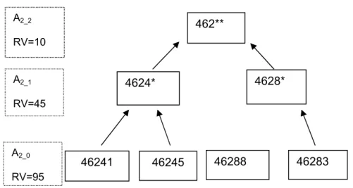
Figure 1. Generalization of race attribute
For each attribute we can define a hierarchy of domain nodes totally ordered using <DG; where the root of the hierarchy represents the most generalized domain, and
the leaf nodes represent the most specific domain (i.e. original domain of the attribute). Figure 1 and Figure 2 provide examples of the domain generalization hierarchies for the race and zip code attributes.
Figure 2. Generalization of the zip code attribute
Direct edges between two nodes are the results of direct generalization produced by applying the generalization function γ; and paths between nodes are implied
generalization between domains produced by a series of composition of the generalization function, denoted by γ+. Each generalization level for an attribute is
A1_2 RV=15 A1_1 RV=35 A1_0 RV=95
White Black Hispanic Asian White Black Other White Other 46288 A2_2 RV=10 A2_1 RV=45 A2_0 RV=95 46241 46245 46283 462** 4624* 4628*
8
labeled with the attribute number x and the generalization level y (Ax_y). The most
specific data for an attribute is labeled with a zero, Ax_0, and as the attribute becomes
more generalized the value increases by one. In Figure 1, the most generalized level is labeled as A1_2.
Full Domain Generalization
As described in [8, 38], several models exist to transform table T to the
k-anonymized view V, including the global recoding. In global recoding the initial values of each quasi-identifier attribute are mapped to new values to satisfy k-anonymization. Several approaches exist for global recoding; see [7, 8] for more information. Using full-domain generalization approach, initial values of each quasi-identifier attribute are mapped to values in the same domain in the attribute domain hierarchy. More formally, let T be a relation with quasi-identifier attributes A1,…An. A full-domain generalization is
denoted by a set of functions, Φ1,…Φn, each of the form Φi : DAi DQi , where DAi<DG
DQi . Φi maps each value “q” from DAi to some value “a” in DQi such that a = q or a
belongs to γ+(q). A full-domain generalization V of T is obtained by replacing the value q of attribute Ai in each tuple of T with the unique value Φi(q) [30, 32]. This is in contrast with local recoding [13, 14, 27], where initial values of an attribute Ai can be mapped to values in different domains in the attribute domain hierarchy. For example, the age attribute value of 15 exists in the 15-20 domain as well as in the 14-18 domain. The general idea of local recoding is to minimize the interval size, which may achieve less information loss due to smaller intervals than global recoding. We address the issues of the same values existing in different domains in the Utility Metric section.
This property allows generalizing attribute domains into higher domains. The hierarchies of an attribute domain generalization can be constructed by progressively mapping the attribute domain values into a higher attribute domain.
9
The race attribute is shown in Figure 1, and the zip code attribute is shown in
Figure 2. It is initially defined at the most specific level of the attribute to be (White, Black, Hispanic, Asian). It was then generalized to the level (White, Black, Other) and then into an even more generalized level (White, Other). The generalization groupings of the race attribute example demonstrate a concept that is critical to our new data content expert based utility measurement, which is that particular values in an attribute are maintained as much as possible even if they exist in multiple generalization levels. For example, the values of White and Black exist in three generalization levels, and the reasoning for this is that those two values in the race attribute have been designated by the data content expert as critical for research purposes. If a generalization level is required to drop one of these critical values, the data content expert considers the information loss to be significant. With that in mind, the assigned utility metric for a generalization level without the data content experts desired values intact will reflect that loss. More details on the calculation of the utility metric are defined in the Utility Metric section.
Related Work
The protection of microdata has been an active research issue [39], and many researchers have been utilizing k-anonymity to protect the identities of the individuals in a database. K-anonymity and the deployment of generalization/suppression to satisfy k-anonymity were originally characterized in [32], and a binary search algorithm to find a single full-domain generalization was described in [30]. New optimization methods were developed in [2, 4, 7, 20, 21, 26]. For example in [20], the authors introduce a class of algorithms for a multi-dimensional data model that produce k-anonymous full-domain generalizations while still maintaining a substantial performance improvement over existing full-domain algorithms.
10
An area of research within privacy protection has been the analysis of k-anonymity, and whether or not it protects the privacy of data. L-diversity, proposed by
[25], suggests that k-anonymity is susceptible to homogeneity of the data combined with the knowledge of the attacker. An examples is that if the attacker knows that a dataset includes all persons in a county, and the data shows that all persons in the datasets with syphilis also have AIDS, and the attacker has external knowledge that his acquaintance Jim, a county resident, has syphilis, the data has revealed to the attacker than Jim has AIDS. As initially described, l-diversity proposes to protect not only the quasi-identifiers,
but provides special attention to a subset of the attributes called sensitive attributes (e.g.
an attribute storing HIV status for a patient, which the patient would not want disclosed) characterized by having at least l well-represented values exist in a set of records that
have the same values for the quasi-identifiers. In contrast to l-diversity, [22] proposes a
concept called t-closeness. This concept is based on the premise that for any equivalence class, which is a set of quasi-identifiers, the distance between the distribution of a sensitive attribute in the equivalence class and the distribution of the attribute in the whole table is no more than a threshold of t.
We consider all attributes in a dataset to be sensitive attributes, so during the anonymization process, our algorithms ensure that we have k records to prevent identity
disclosure. Even though our anonymized dataset may not satisfy t-closeness, we ensure that we have at least k records for each of the “sensitive” attributes as classified in [25]. An attacker may have external information about any subset of attributes within a dataset, and so any attribute must be treated as a possible contributor to identity
disclosure, as illustrated by the two attributes Resident County and syphilis status in the prior example. To achieve k-anonymity, there must be at least k records with any
11
from some subset of attributes that have been categorized as identifiers or quasi-identifiers.
Among studies of the utility of the data after anonymization, the research of Xu et al. [28] is one of the few studies that emphasized the need to build utility aware
anonymization in terms of weights among individual attributes. The example they provide highlights the difference in importance that exists between age and zip code attributes when conducting a study for disease analysis. More precisely, age has more importance in this type of study. Therefore, it makes sense to try to minimize the level of generalization of age when compared to zip code during the transformation process. It should be noted that the weights are not intended to create different anonymized
datasets for each type of user, but instead provide weight on attributes that are generally more important for the majority of users of the data. For this aim, an attribute weight has been introduced in the utility metric they proposed; although it has been set to one all across the attributes when actually implemented. The utility metric obtained corresponds to the sum of the weighted utility of each attribute. The utility metric, also called
normalized certainty penalty, is expressed in terms of the loss of information generated
by the generalization process. In a case of a numeric quasi-identifier attribute Ai whose initial domain Di is generalized to domains Di_0, Di_1, ... Di_m, the loss of information is
expressed in terms of the sum of the ranges of each sub domain Di_j normalized by the
range of the initial domain. Di. Similar reasoning can be extended for categorical
attributes.
In other works of k-anonymization such as in [7, 16, 21] the authors have also introduced utility matrices to guide the transformation process; but did not take into account the importance of the attributes. For example in [7], the discernability model is
introduced to measure the information loss for each attribute Ai, by assigning a penalty to each tuple in the table based on the number of tuples having the same generalized
12
sub-domain Di_j. In the work described in [14], the normalized average equivalence class
size is introduced. For each quasi-identifier attribute Ai, the information loss is expressed
in terms of the number of tuples in the table divided by the number of group-bys for the attribute Ai generated in the next generalization level.
In the work described in [12], the authors propose to release frequency related information about the data called marginals. For example, if there are five people in a zip code that are forty years of age, the authors will release a table with an entry of forty with a count of four. The determination of what marginals are released is dependent on an entropy measure and not based on the needs of the researcher who wants to mine that data. The concept of a normalized certainty penalty (NCP) is introduced in [10, 28] to capture information loss as the data is generalized into intervals, therefore losing
accuracy in query answering. For example, a user may want to know how many 18 year old men purchased beer and diapers in 2005, but may only be able to count men ages 16 to 20 years old if age has been aggregated into five year domains in the dataset. For all numerical attributes, Ai, from table T, NCP is defined as
| |
where |Ai| is defined to be the . . , i.e. the range of all tuples
on attribute Ai. The numerator contains that variables yi, and zi, which are the
generalized values for xi. Finally, wi reflects the weight of the utility for attribute Ai as
compared to the other attributes in the dataset.
Categorical attributes follow the following formula for the NCP:
| |
where the size(u) is the number of common descendants and |A| is the number of distinct values for attribute A. The NCP is an interesting concept, but its limitation is that
13
it does not take into account the importance of particular values in the dataset that have been identified by the data content expert as critical to the analysis of the researcher. In the next section, we present our utility metric that builds upon aspects of the NCP, but also penalizes a particular generalization level of an attribute if the critical values of that attribute have been generalized. The data content expert, who is very familiar with the needs of the researchers receiving the data, pre-defines these critical data values in rules that may be a value like “white, or black” for a categorical attribute like race, or a range of numbers like 12-18 for age is well accepted as “adolescent.” If these values are not present in a particular generalization level, then the information loss increases and the penalty also increases.
Utility Metric
We propose that the data curators should have more control defining the utility of the attributes and how they relate to the overall content of the data that is contained in the datasets that they own. The expertise of the data researchers provides an
understanding particular to critical thresholds in the data that should be maintained through the anonymization process, so that the meaning of the data is well maintained. In [27, 28], a new utility measurement called the research value (RV) was introduced to encapsulate the utility of the each attribute with respect to the following conditions:
Significance of the attribute relative to the other attributes;
The distinct number of elements in a group at a particular generalization level;
The number of records that exist for each group in a generalization level;
The number of data constraint rules that are maintained in that generalization level.
A data constraint rule (DCR) defines groupings of data or ranges of data that, if maintained, help to maximize the meaning of the data for the end researcher. The data
14
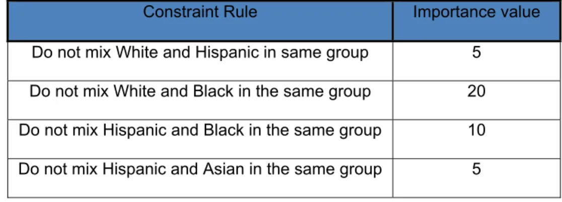
constraint rules can exist in two forms depending on the data type of the attribute: categorical or continuous. Categorical attributes use data constraint rules that preserve distinctions between data values or between data value domains. When all of the data constraint rules are satisfied at a particular generalization level of an attribute, the value of the data constraint rule in the RV is the sum of all possible importance values divided by the sum of all the importance values in the raw dataset, which would be one. Any generalization that violates such a constraint rule would be penalized by multiplying the generalization string’s total research value with a value less than one. Using the race attribute as an example, the data expert may assign the following importance values to the elements that exist for race in a database:
Table 1. Possible Data Constraint Rules for the Race Attribute Constraint Rule Importance value Do not mix White and Hispanic in same group 5
Do not mix White and Black in the same group 20 Do not mix Hispanic and Black in the same group 10 Do not mix Hispanic and Asian in the same group 5
If a generalization level violated the mixing of Hispanic and Black individuals, then the data constraint portion of the RV would be 30/40 = 0.75.
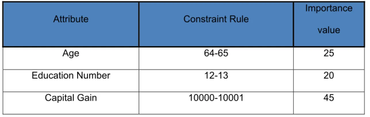
For a continuous attribute like age, the data constraint rules could define
inflection points of ages that would be important for someone who is interested in mining the data. For example, preserving a distinction between age 20 and 21 years may be important to a researcher examining alcohol use, since drinking alcohol usually becomes legal on a person’s 21st birthday. Similar to the continuous data constraint rules, the
15
importance values assigned for each of the ranges of values for an attribute are normalized to one.
Table 2. Possible Data Constraint Rules for Numerical Attribute
Attribute Constraint Rule
Importance value
Age 64-65 25
Education Number 12-13 20 Capital Gain 10000-10001 45
The research value (RVk) of a numerical attribute x at generalization level k is
defined to be:
RV w ∑ R NR
∑ R NR
∑ DR ∑ DR
where wx is defined to be the importance weight of attribute x in reference to the other
attributes in the dataset. The numerator ∑ R NR is the sum of the number of elements within each sub-group i times the range of values for those elements in the ith
group at the most specific generalization level of attribute x. ∑ R NR is the sum of the number of elements within each sub-group i times the range of values for those elements in the ith group at the kth generalization level of attribute x. Finally, the data
constraint rules portion of the equation is the ratio of the sum of the data constraint rules that exist at the kth generalization level, ∑ DR , divided by the total value of all the data
constraint rules at the most specific generalization level, ∑ DR . Each dataset has an inherit value even if all of the data constraint rules are broken during the merging of two clusters, so to resolve this, the data owner has the ability to add a base value to the data constraint ratio, so that it does not zero out a RV if all of the rules are broken. The weight
16
calculation of each attribute can be determined by establishing a correlation matrix among attributes using the original raw dataset. The total sum of all the weights is normalized to be 1. If an attribute does not correlate highly with any other attribute, then that attribute is considered to be an independent attribute and will be assigned a higher weight. On the other hand, if an attribute is highly correlated with the other attributes, then it will be assigned a lower weight. As the number of attributes increases, the
complexity of determining the correlations between attributes increases dramatically. For the experiment we describe in this paper, the data expert manually assigned weights for each of the attributes in both the MCPHD and Adult datasets, but the proposed utility metric to calculate the RV values was used at each generalization level of the two datasets.
For categorical attributes in a dataset, the research value (RVk) of attribute x at
generalization level k is defined to be:
RV w |A |
|A |
∑ DR ∑ DR
where all the elements are defined to be the same as those for the numerical attributes, except for the |A |
|A | ratio which is defined the number of unique elements at generalization
level k divided by the number of unique elements defined at the most specific generalization level of the attribute.
To demonstrate the calculation of the research value for the kth level of attribute x
containing numerical data, the following example is presented. The weight of the attribute x is calculated to be 0.2; there are three groups in this generalization level with 25, 45 and 55 elements in each group spanning 10, 15 and 25 values, respectively. The most specific generalization level of this attribute has 125 elements with a group
spanning of 1. The sum of the data constraint rules, which include the base value as determined by the data owner, that exist at the kth level is 50, while the sum of the data
17
constraint rules at the most specific generalization level is 100. Given all of these values, the research value for the kth level of attribute x is determined as:
0.2 125 1
25 10 45 15 55 25
50
100 0.0054
At the most specific level, the RV of an attribute is equal to wx. It becomes
apparent that as one moves to more generalized levels within an attribute, the
denominator will continue to grow, and thus the RV value will continue to decrease. As the number of elements increases within a sub-group at a particular generalization level for an attribute, the chances are greater that those set of values will produce a
measurable pattern during data analysis. In contrast, if the range of values within a sub-group is very large, then the chances of producing a measurable pattern in the dataset decrease.
It is important to note that given two attributes Am and An such that Dm_0≤ Dn_0,
then the initial importance status is not necessarily maintained as attributes Am and An
are generalized. That is, Dm_i≤ Dn_j where i<j does not always hold in the general case.
This is a result of the data constraint rules defined for a particular attribute, and how the generalization levels are defined for those attributes. Informally, the partial order
between research values allows for flexibility in defining domain hierarchies for each attribute and the ability to re-evaluate the utility of the attribute and its importance with respect to the other attributes as the attributes undergoes global recoding. Compared to the information loss defined in [10], the research value metric can be regarded as an opposite metric, wherein the more the attribute undergoes transformation, the less research value it will have.
To optimize the final overall utility of the transformed data using the research value metric, two alternative algorithms are proposed:
18
Optimization of the overall research value of the dataset after generalization by maximizing the overall sum of the research values of the transformed attributes. We call this option global research value optimization
Optimization of individual attribute research value, by maximizing the individual research value of each transformed attribute. We call this alternative local
research value optimization
It should be noted that the research values used by these proposed algorithms were manually calculated by the content expert, and that our future work will be to automatically generate the research values of the attributes.
Methodology
In this section, we will describe the two algorithms that address the global research value optimization and the local research value optimization and the datasets
that were used for running experiments on the algorithms. DataSets
For this project, we utilized two datasets, the public Adult Census data from the UC Irvine machine learning repository [29], and the proprietary death certificate dataset from the Marion County Public Health Department (MCPHD) of Indianapolis, Indiana. We included the Adult Census dataset in order to compare our proposed algorithms against existing methodologies, since the MCPHD is not available for public download, and the Adult Census dataset is the gold standard for gauging anonymity techniques.
The Adult dataset was configured in a similar manner to [41] using 30,162 tuples and eight attributes (age, work class, education number, marital status, occupation, race, sex and native country). Age and education number were used as numeric values, while the remaining attributes were used as categorical attributes. Work class and marital status used a three level hierarchy structure. For the other categorical attributes, a two
19
level hierarchy was used with the most specific level having all values, and the second level was set to “ALL,” (i.e. complete suppression).
For the Marion County Health Department’s death certificate dataset (a total of 216,000 records) comprised of 76 attributes was paired down to 36 attributes based upon their utility for data mining. These attributes include: race, sex, college education, cause of death, etc are listed in Table 3. For each attribute, we created n levels of
generalization, where n ranged from one to six. The original version of the MCPHD
dataset contained a wide range of values in each attribute. This variety produced many outlier values that needed to be reclassified for categorical attributes, or removed in the case of numerical data after performing a distribution analysis of each attribute to identify outliers.
Table 3. Marion County Public Health DB Attributes Marion County Public Health Department Database Attributes
Race, Sex, Age in Days, College, Industry, Autopsy, Census Tract, Cause of Death Certifier Type, Citizenship, City of Birth, Date of Birth, Date of Death, Disposition Method, Education, Farm, Informant Relationship, Injury AM/PM, Injury Census, Injury County Code, Injury Date, Manner of Death, Marital Status, Military Motor Vehicle Accident, Occupation Category, Occupation Code, Place of Death City, Place of Death Code, Place of Death State, Place of Death Zip, Pregnant, State of Birth, US Vet, Zipcode, Injury Time, Time of Death
These identified outliers were then recoded to a general category within the attribute. As described above, every level of generalization for each attribute was
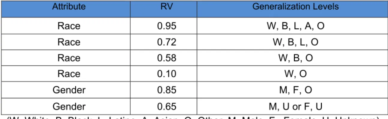
assigned a research value (RV), which ranged from zero to one hundred (i.e. normalized values). Table 4 demonstrates another generalization example of the two attributes (Race and Gender), and the corresponding research values for each level of generalization within the attribute.
20
Table 4. Research Value Examples
Attribute RV Generalization Levels
Race 0.95 W, B, L, A, O Race 0.72 W, B, L, O Race 0.58 W, B, O Race 0.10 W, O Gender 0.85 M, F, O Gender 0.65 M, U or F, U
(W=White, B=Black, L=Latino, A=Asian, O=Other, M=Male, F =Female, U=Unknown)
Data Preparation
Using the MCPHD and the Adult census raw datasets, a perturbed dataset was created by running a SAS® script that formatted the data into generalization columns. For each attribute, x columns were created based upon the number of levels of
generalization each attribute contains, as discussed in the previous section. In Figure 1, we can see how the race attribute, which has three generalization columns, will be created (A1_0, A1_1, and A1_2). In the A1_0 column, all of the records will contain either
“White,” “Black”, “Hispanic”, “Asian.” In the A1_1 column all records containing either
“Asian” is abstracted into “Other”; and in A1_2 column all records containing either
“Black”, “Hispanic” or “Other (from the previous level) are abstracted into “Other.” The last level (not shown in Figure 1 and 2) is the most general level with a zero research value, where all records contain the same value, “any”, for the generalized attribute. Throughout the hierarchy creation process, no attribute values were allowed to be in two groups at once. For example, a generalization of the age attribute could not have
overlapping groupings, like age 13-17 and age 15-22. When values are allowed to cross groupings, it makes it very difficult to discriminate what grouping of a particular value (i.e. 15 in this example) is responsible for a pattern in the dataset. In effect, the groupings for age would range from 13-22, because you could not assert if 15 was in the 13-17
21
grouping, or the 15-22 grouping; thus the utility of the dataset has been decreased. This is a weakness of the local recoding methodology. Publications using local recoding where values are allowed to cross groupings during the anonymization process include [3, 4, 13, 42]. This process was repeated for all thirty attributes in the MCPHD dataset and then for the Adult census dataset.
After all thirty attributes of the MCPHD had been generalized, multiple
combinations of those thirty attributes were created to test the effectiveness of the two proposed algorithms. A combination contained as little as three attributes and up to the maximum of thirty attributes. The criteria for the selection of the attributes that were selected for each combination fell into two categories: 1) Random or 2) Maximum number of generalization levels. The maximum number of generalization levels approach would examine two attributes A1 and A2 and select A1 if it had more
generalization levels than A2, or vice versa. In the case where A1 and A2 had the same
number of generalization levels, then one would be selected randomly. The random combinations were labeled as ri (e.g. r03 and r08), which indicates a random selection of i attributes from the original pool of thirty attributes. The maximum combinations were labeled in a similar manner mi (e.g. m03 and m08). For the Adult dataset, all of the attributes were used in during the testing phase of the algorithms.
Algorithms
To ensure that a dataset is k-anonymous, it is critical to test the worst case scenario for the data, which in this case is a combination of all possible attributes being searched in a single query. This is due to the fact that as the number of attributes that are combined in a query increases, the chances of k-anonymity being violated also increases. Herein after we represent this combination of attributes as a string called generalization string A1_1A2_2…Am_n composed of the combination of the individual
22
attribute generalization level strings Ai_j. For example, the race and zip code attributes
would create generalization strings like A1_0A2_0, A1_0A2_1, A1_1A2_0, etc.
The aim is to efficiently compute a dataset generalization string that optimizes (globally or locally) the overall research value of the transformed view V. Let us call this string globally (resp. locally) optimized generalized string.
One problem with this strategy is that a dataset with large numbers of attributes will create millions of possible combinations of generalization strings. From efficiency perspective the bottleneck point for either one of the alternatives is the computation of the frequency set for any dataset generalization string, as it involves a database call to compute a select-group-by SQL statement.
Given a set of attributes A = A ,A ,…,A and a set D of attribute domain
generalization hierarchies, the initial number of dataset string generalizations is function of the number “n” and the number of levels of each attribute domain hierarchy in D. Therefore to reduce the number of initial dataset generalization strings, we need to reduce either the number of initial attributes and/or the hierarchy depth of the attributes. The pre-pruning phase addresses both options.
Pre-Pruning
The strategy employed in the pre-pruning phase is supported by the following properties also used in [14]. The first property called the generalization property states that if two sets of attributes P and Q have their domains satisfying DP≤ DQ, and if T is
k-anonymous with respect to P; then T is k-k-anonymous with respect to Q.
The second property called subset property states that if T is k-anonymous with
respect to a set of attribute P, then T is also anonymous with respect to any subset of P. Using the negation of the subset property we can infer that if T is not
k-anonymous with respect to an attribute in A, then it is not k-k-anonymous with respect to any superset obtained by combining the attribute with the other attributes of A. Using the
23
negation of the generalization property we can infer that if T is not k-anonymous with respect to Ai_j then it is not k-anonymous with respect to Ai_l such that l<j. The outline of
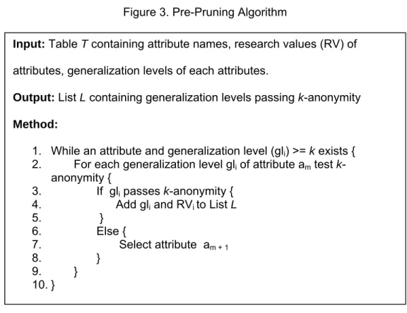
the pruning strategy is depicted in Figure 3.
Figure 3. Pre-Pruning Algorithm
The pre-pruning strategy uses the negation of both properties, by checking for each attribute whether or not it satisfies k-anonymity (Line 3). If it does not, then it can be pruned from the composition of the initial generalization string set. To account for the existence of different domains for each attribute, we refine the pruning process to prune for each attribute any generalization domain that does not meet k-anonymization. For example, in Figure 1, if attribute A10 does not meet the k-anonymization threshold but A11
and A12 do, then the domain hierarchy of attribute A1 will be trimmed to include only the
top two levels; and therefore only A11 and A12 will be used in generating the set of initial
dataset generalization strings. If an attribute A1 fails k-anonymity at the most generalized level, then that attribute is removed from the dataset, because it would cause other attributes that were combined with A1 to also fail k-anonymity. The benefit
Input: Table T containing attribute names, research values (RV) of
attributes, generalization levels of each attributes.
Output: List L containing generalization levels passing k-anonymity
Method:
1. While an attribute and generalization level (gli) >= k exists {
2. For each generalization level gli of attribute am test k
-anonymity {
3. If gli passes k-anonymity {
4. Add gli and RVi to List L
5. } 6. Else { 7. Select attribute am + 1 8. } 9. } 10. }
24
of this pre-pruning process is a more efficient k-anonymity algorithm by minimizing the number of calls to the database to test the generalization strings for k-anonymity.
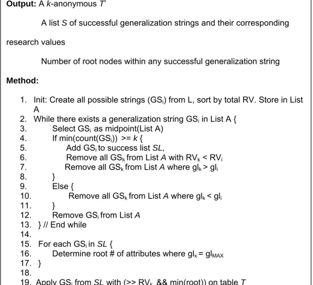
Global Optimization of the Utility Metric
The aim is to compute the dataset generalization string that meets the
k-anonymity threshold and have the best global research value. The global research value is computed by summing all of the research values from each respective attribute in the successful generalization string. This method requires that the research values of all combinations of the attributes’ generalizations be calculated. This may produce a very large number of generalization strings, as is the case for the MCPHD dataset, but the pre-pruning eliminates a large portion of the strings that do not satisfy k-anonymity. To minimize the number of database calls, we deploy a binary search over the list of all dataset generalization strings sorted in ascending order on their global research value. At each step of the binary search, we apply several strategies to minimize the number of generalization strings that need the computation of the frequency set. The pruning steps depend on whether the selected generalization string fails the k-anonymity test. The details of the global optimization algorithm are shown in Figure 4.
For the case of a success, the generalization string is added to the list of successful strings SL and the pruning strategies are applied. The first pruning strategy eliminates all generalization strings with a global research value less than the successful string. The second pruning strategy eliminates all generalization strings that are more general that the successful strings. A generalization string is considered to be more general if all of the component attributes of that string have a generalization level glk > gli
where i is the generalization level of the current string, and k is the generalization level of
25
For the case when the current generalization string fails, then the only pruning strategy that applies is to remove all generalizations strings that are more specific than the current string.
Figure 4. Global Optimization Algorithm
The binary search process is repeated for the remaining list of non- pruned generalization strings until no more strings are left to be analyzed. If multiple successful generalization strings were found after running the algorithm, all having similar research values, then it would be at the discretion of data content expert to select a generalization string that would be most beneficial from the end-user perspective. The number of root
Input: List L
Output: A k-anonymous T’
A list S of successful generalization strings and their corresponding
research values
Number of root nodes within any successful generalization string
Method:
1. Init: Create all possible strings (GSi) from L, sort by total RV. Store in List
A
2. While there exists a generalization string GSi in List A {
3. Select GSi as midpoint(List A)
4. If min(count(GSi)) >= k {
5. Add GSi to success list SL,
6. Remove all GSk from List A with RVk < RVi
7. Remove all GSk from List A where glk > gli
8. } 9. Else {
10. Remove all GSk from List A where glk < gli
11. }
12. Remove GSi from List A
13. } // End while 14.
15. For each GSi in SL {
16. Determine root # of attributes where glx = glMAX
17. } 18.
26
nodes (most specific levels of an attribute) is determined to provide the data content expert the ability to choose from multiple success strings after the anonymization process is complete.
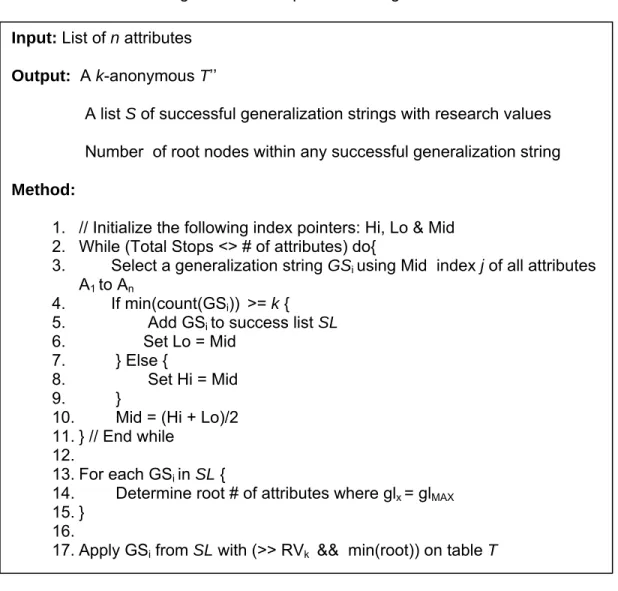
Local Optimization of the Utility Metric
The objective of the local optimization approach is to achieve K-anonymity with optimum RV values for each attribute (i.e. local). As opposed to the global optimization approach where the focus is to find the best RV combined over all attributes, the aim of this approach is to balance the global RV value between the attributes. In other words, finding generalization strings that minimize the cases where generalization strings include very specific attributes at the expense of most general attributes. For example, using attributes race and zip code in Figures 1, the best generalization string using the global strategy would generate the generalization string A1_2A2_0 (combined RV=0.90)
while the local strategy may generate the generalization string A1_1A2_1 (combined
RV=0.50).
Unlike the global approach, the local approach does not use a combined list of all possible strings to select a generalization string for k-anonymity testing. Instead, each attribute is regarded separately (As shown in Figure 5), and at each step, a
generalization level within each attribute is selected and combined with the other selected generalization levels of the other attributes in order to create a combined generalization string to be tested for K-anonymity. If that particular generalization string succeeds, then the next selected generalization level in each attribute moves half way up the height of the attribute towards the more specific data of an attribute (i.e. the data is not grouped or suppressed). On the other hand, if the generalization string fails, then the next selected generalization level selected in each attribute moves half way up the height of that attribute towards the more general data. This continues until it is not possible to move in all of the attributes that compose the generalization string. If the
27
current generalization string passes k-anonymity, then the current string is added to the success list SL along with its total research value. No pruning occurs in the local
optimization algorithm, but a hybrid version of the local optimization as described in the next section does use pruning.
To facilitate a binary search in each of the attributes of the generalization string, we utilize pointers to maintain the current selection level of the attribute, and also the highest and lowest points still available for selection.
Figure 5. Local Optimization Algorithm
This procedure continues until the current selection level does not change during an iteration, which is classified as a stopping condition for that attribute. When all of the attributes have met their “stopping condition,” the algorithm terminates. At this point,
Input: List of n attributes
Output: A k-anonymous T’’
A list S of successful generalization strings with research values
Number of root nodes within any successful generalization string
Method:
1. // Initialize the following index pointers: Hi, Lo & Mid 2. While (Total Stops <> # of attributes) do{
3. Select a generalization string GSi using Mid index j of all attributes
A1 to An
4. If min(count(GSi)) >= k {
5. Add GSi to success list SL
6. Set Lo = Mid 7. } Else {
8. Set Hi = Mid 9. }
10. Mid = (Hi + Lo)/2 11. } // End while
12.
13. For each GSi in SL {
14. Determine root # of attributes where glx = glMAX
15. } 16.
28
similar to the global approach, all of the success strings are examined for any roots. The aim is to eliminate success generalization strings with attributes at the most general level. The generalization string with the greatest research value and fewest number of root attributes would then be applied against the raw database to ensure anonymity while still maintaining some of the utility of the data.
Hybrid Utility Algorithm
The hybrid approach is a combination of the local approach and the global approach that takes advantage of the quick examination of strings via the local algorithm and then uses the wider scope of the global algorithm to identify any remaining success strings. Unlike the local optimization approach, the hybrid optimization makes use of the list of all possible generalization strings for a dataset, and pruning of those strings as the algorithm executes. It starts of using the local algorithm until all of the high and low pointers for all of the attributes are equal. Once this point is reached, if there are any entries left in the remaining list of generalization strings, the global algorithm is then called until no entries exist in that list.
Distributed Version of the Global Optimization
As described in Global Optimization Algorithm section, the global approach assumes that all possible generalization strings are generated a priori and provided as an input (residing in main memory) for the algorithm. This assumption generates implementation issues as soon as we have a number of attribute combinations greater than twelve. To address this issue we propose a distributed version of the algorithm that leverages the subset property described in Global Optimization Algorithm section. The main idea of the distributed version of the algorithm is to decompose the generalized string into subsets of generalization strings that can fit in memory; and then run the generalization algorithm described in the Global Optimization Algorithm section on each of the subsets looking for successful strings within those subsets. Once all of the strings
29
have been analyzed for a particular subset, the algorithm then starts on the next subset. After all of the subsets have been analyzed, the successful strings from all of those subsets are combined and then tested for k-anonymity. Any successful strings from these combined strings are then tested for any attributes that are at the root level and the string with the highest RV is applied to the raw database. Since the datasets we used only produced successful generalization strings using three and six attributes, the distributed approach was not needed, but as we increase the number of attributes beyond twelve, the distributed approach will be needed to ensure the scalability of the algorithm.
Experiments
Algorithm Performance
The performance of the local optimization algorithm is log2(max height of n
attributes in generalization string) is based on the fact that the local algorithm uses a binary search technique, and it repeats until no more moves are allowed in any of the attributes. For the global optimization algorithm, the performance of the algorithm is log2
(generalization of all strings).
Utility Measurement MCPHD Dataset
The global optimization utility metric algorithm was tested using multiple k values on the Marion County death certificate database to test how the algorithms would perform. For this dataset, the research values were established by the data content expert and not the utility function. Currently, we are testing our algorithms with the research values generated using our utility function to compare the outcomes from the values generated by the data content experts and our new utility function. We plan on submitting this as a future publication.
30
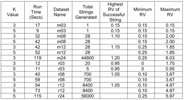
Results from the MCPHD dataset using k values of three and five with multiple
combinations of attribute are shown in Table 5. As the k value increases, the amount of
successful records drops off dramatically (in most cases, there were zero successful strings found) for datasets that contained more than twenty-four attributes. So the data is not shown for those cases. We will discuss the possible reasons for no successful generalization strings using the MCPHD dataset. In Table 5 and Table 6, any empty entries found in the tables indicate that no successful generalization string was found for that run. Datasets mYY contain the attributes that have the most generalization levels within the attribute, while the rXX datasets have randomly selected attributes. m12 had fewer total strings due to the fact that the pre-pruning phase eliminated a considerable amount of generalization levels in the attributes for that dataset, and thus the total number of combinations of generalization strings was less than the r12 for example.
Table 5. Global Optimization Utility Algorithm
K Value Time Run (Secs) Dataset Name Total Strings Generated Highest RV of Successful String Minimum RV Maximum RV 3 8 m03 1 0.15 0.15 0.15 5 9 m03 1 0.15 0.15 0.15 3 41 m08 28 1.10 0.15 2.00 5 41 m08 28 1.10 0.15 2.00 3 49 m12 28 1.00 0.25 1.85 5 49 m12 28 1.00 0.25 1.85 3 25764 m24 44800 1.2 0.25 6.03 3 17 r03 20 0.95 0 1.75 5 13 r03 5 0.48 0 0.995 3 270 r08 700 1.00 0.10 3.67 5 282 r08 700 1.00 0.10 3.67 3 2459 r12 8400 1.00 0.10 4.87 5 2498 r12 8400 1.00 0.10 4.87 5 14961 r24 24 0 6.07
31
Table 5 shows the different runs that use K values of three or five. Within each run, the highest total research value for the dataset is listed along with the maximum and minimum research values for the run. The maximum research value corresponds to an anonymized dataset that contains attributes that all contain their most specific
generalization levels, while the minimum research value corresponds to an anonymized dataset that contains attributes that all contain their most generic generalization levels. The empty entries in the highest RV of a successful string column indicate that no selected generalization strings passed the k-Anonymity test.
Table 6 shows the results of running the local optimization utility algorithm under the same k value conditions as the global algorithm. This table contains the same fields as that of the global optimization utility algorithm to allow for comparisons of the two algorithms on the same datasets.
Table 6. Local Optimization Utility Algorithm
K Value Run Time (Secs) Dataset Name Total Strings Generated Highest RV of Successful String Minimum RV Maximum RV 3 17 m03 1 0.15 0.15 0.15 5 9 m03 1 0.15 0.15 0.15 3 32 m08 28 1.10 0.15 2.00 5 42 m08 28 0.15 2.00 3 42 m12 28 1.15 0.25 1.85 5 52 m12 28 0.25 1.85 3 119 m24 44800 1.20 0.25 6.03 3 12 r03 20 0.95 0 1.75 5 11 r03 5 0.95 0 0.95 3 40 r08 700 1.05 0.10 3.67 5 59 r08 700 0.10 3.67 3 54 r12 8400 1.05 0.10 4.87 5 73 r12 8400 0.10 4.87 5 115 r24 56000 0.25 5.97
32
Adult Census Dataset
As a means to show how our algorithm performs against existing utility methodologies, our two proposed algorithms were run using the public Adult census dataset using a range of k values (k=3, k=5 and k=10).
Unfortunately, the local optimization algorithm was not able to find any solutions using the Adult DB, and this will be addressed in the next section. We then ran the Bottom Up algorithm as defined in [42] using the same three values of k to compare with our methodology and utility metric. The authors of [29] presented a Top Down and Bottom Up algorithm, but both showed very similar results, with the only difference being the execution time, which was not a concern for us in this exercise. For this dataset, we did use our new utility function to establish the research values for each of the attributes and the generalization levels of those attributes.
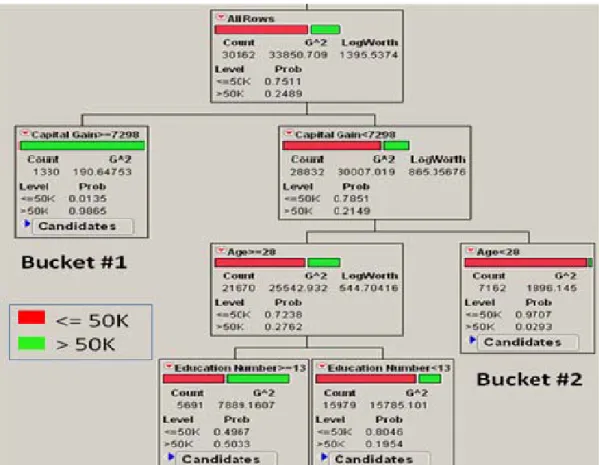
In order to examine the effects of the anonymization process, we used recursive partitioning (RP), which is a multivariable technique that is used to find patterns in large datasets, on the raw Adult dataset to see which of the attributes were most responsible for differentiating individuals who make <=50K or >50K in yearly salary. Salary was chosen, because it is the attribute of interest in the Adult dataset for analysis. As seen in Figure 6, out of the original 30162 records, 75% of the individuals had a yearly salary of <=50K and 25% had a salary >50K.
33
Figure 6. Raw Adult Dataset Recursive Partitioning
The three attributes that significantly differentiated the two salary groups are Capital Gain, Age and Education Number. Bucket #1 indicates that when an individual has Capital Gains >=$7298, 98% probability of the 1330 individuals having a yearly salary of >50K. On the other hand, bucket #2 shows that when Capital Gains <$7298 and Age is <28 years old, 97% probability of 7162 individuals having salaries <=50K.
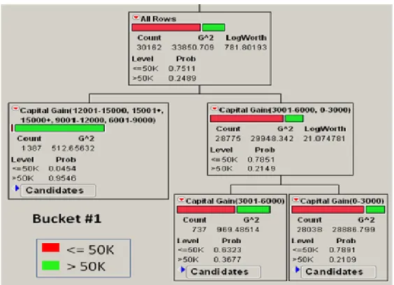
After running the global optimization algorithm using a k value of 5, the anonymized dataset was analyzed using recursive partitioning and it produced the breakdown as shown in Figure 7. Bucket #1 shows that when the Capital Gain is >=$6001, 95% probability of the 1387 individuals having a yearly salary of >50K. The Bottom-Up algorithm with a k value of 5 was also run against the Adult dataset and the recursive partitioning results are shown in Figure 8. Bucket #1 has a mixture of Capital Gains that range from zero to $15,000+, so no conclusions can be drawn from
34
this bucket. When the Education Number is Pre-college for all values of Capital Gains, 86% of the 18686 individuals from the 516 clusters in bucket #2 have Salaries <=50K.
Figure 7. Global Optimization RP using k=5
Both algorithms were also run on the Adult dataset using a k value of 10. The Global Optimization algorithm did not produce a valid solution where the Salary attribute is not generalized to a value of both <=50K and >50K. On the other hand, the Bottom-Up algorithm produced a result that is found in Figure 9.
As in the previous runoff of the Bottom-Up algorithm, Bucket #1 had Capital Gain represents a full range of values. Therefore no conclusion can be determined. Bucket #2 has a full range of Capital Gain values and Education Numbers of Pre-College have 86% of the 18686 individuals have a Salary <=50K. When the value of k was raised to be 10, neither the local nor the global optimization algorithms could produce a solution where the salary attribute did not contain the most generalized values for the salary (i.e. salary= “both”). In contrast, Figure 9 shows that the Bottom Up algorithm was able to find
35
a solution. As present in the k=5 solution, Bucket #1 had the full range of Capital Gain values. Bucket # 2 represents Capital Gain values <$7000 that have 86% of 20,000+ individuals having a Salary <=50K.
36
Figure 9. Bottom-Up Recursive Partition k=10
Discussion
The goal of the algorithms described in the previous section provide the optimization of data utility in a dataset while still protecting the anonymity of the individuals stored in that dataset. As shown in Table 5 and Table 6, the global
optimization utility metric algorithm and the local optimization algorithm are extremely close in terms of the highest research value of the successful strings.
Marion County Public Health Department
For the Marion County Health Department database, the local optimization algorithm (Table 6) performed better than the global optimization algorithm when you compare the highest successful research value discovered relative to the maximum total research value using the mXX datasets, where XX was under 12 attributes. As the