Parallel Algorithms for Counting Problems on Graphs Using Graphics Processing Units

(1)

UNIVERSITY OF OKLAHOMA GRADUATE COLLEGE

PARALLEL ALGORITHMS FOR COUNTING PROBLEMS ON GRAPHS USING GRAPHICS PROCESSING UNITS

A DISSERTATION

SUBMITTED TO THE GRADUATE FACULTY in partial fulfillment of the requirements for the

Degree of DOCTOR OF PHILOSOPHY By AMLAN CHATTERJEE Norman, Oklahoma 2014

(2)

PARALLEL ALGORITHMS FOR COUNTING PROBLEMS ON GRAPHS USING GRAPHICS PROCESSING UNITS

A DISSERTATION APPROVED FOR THE SCHOOL OF COMPUTER SCIENCE

BY

Dr. Sridhar Radhakrishnan, Chair

Dr. Suleyman Karabuk

Dr. John K. Antonio

Dr. Sudarshan Dhall

(3)

(4)

(5)

Acknowledgements

First, I would like to sincerely thank my research advisor, Professor Sridhar Radhakr-ishnan, for inculcating in me a zeal to explore the intricacies of computer science, for encouraging me to work in the forefront of technological advancements, for his guid-ance and unconditional support during all these years of graduate school, and for being a excellent mentor; I am grateful for having the opportunity to work with him. I would also like to thank Dr. Suleyman Karabuk for being in my committee as the external member and providing valuable insights in many research meetings right from the beginning of this work. It has also been a wonderful learning experience while working with Dr. John Antonio on many of the research problems. Also other members of my dissertation committee Dr. Sudarshan Dhall and Dr. S. Lakshmi-varahan have been always encouraging. In addition I had the privilege of working with Dr. Deborah Trytten and Dr. Changwook Kim; teachers from whom I learned the art of communication and conveying ideas.

The School of Computer Science at OU has provided me with great learning experiences and I leave with better education, insight and more surety as an individual and professional in the field. I would like to thank all the faculty and the wonderful staff, specially Barbara, Chryl, Emily, Virginie, Jonathan and Jim Summers, who make this a great learning center.

I also express my gratitude to fellow graduate students and colleagues who made every moment at OU worthwhile. I would like to thank all people associated with Dr. Radhakrishnan’s research group, Chandrika Satyavolu, Yuh-Rong Chen, Asif M. Adnan, Khondker Shajadul Hasan, Sourabh Joshi, Michael Nelson, Yiming Xu, Wei Guo, Ashwin Badri, Mahendran Veeramani. Also thanks to some great people whom

(6)

I have had the privilege to know and associate with during my time at the University of Oklahoma: Harshvardhan Singh, Raghav Pant, Nehul Shah, Syed Naveed Hussain Shah, Shohrab Hossain, Rahul Shukla and all the CSGSA committee members. I would also like to thank my friends from Buffalo, Debarshi Indra, Debmalya Das Sharma, Divya Shankar; my college friend Niladri Kundu, school-mate Ambarish Banerjee and senior from school Swapnoneel Roy.

I would also wholeheartedly like to acknowledge the love and support of my family: my father, late Mr. Ranjit Kumar Chatterjee, my mother Mrs. Subhra Chatterjee; my aunt Ms. Kalpana Mukherjee; my brother, Dr. Anindya Chatterjee and sister-in-law Dr. Allison Chatterjee; my sister-in-laws, Mr. Murari Mohan Banerjee and Mrs. Santwana Banerjee; who have been a constant inspiration, and also my grandparents, aunts, uncles, and cousins everywhere; I could not have accomplished this without you.

Finally, and most importantly, I would like to put in a special note for my wife, Debasmita, whose constant encouragement made this work possible. Without her sacrifice and dedication, this journey would have been incomplete. It is my honor and privilege to find a friend and soul-mate like her, who with her honest feedback and appreciation has made this pursuit of education worthwhile.

(7)

List of Tables

2.1 Properties of levels of memory on GPUs (NVIDIA Corporation, 2010) 15 2.2 Architecture Comparison of Different Nvidia GPUs (NVIDIA

Corpo-ration, 2010) . . . 16

2.3 Number of Memory Transactions on different GPUs (NVIDIA Corpo-ration, 2010) . . . 22

3.1 Distribution of nodes in the banks . . . 31

3.2 S-UTM for even number of nodes . . . 32

3.3 S-UTM with load balanced approach for even number of nodes . . . . 32

3.4 S-UTM for odd number of nodes . . . 32

3.5 S-UTM with load balanced approach for odd number of nodes . . . . 32

3.6 Comparison of time complexity for operations on graphs using different data structures . . . 41

3.7 Comparison of memory requirements for the different data structures 45 3.8 Comparison of space requirements . . . 47

4.1 Architecture Comparison of Different Nvidia GPUs . . . 58

4.2 Maximum size of graphs on different GPUs . . . 59

5.1 Real World Graphs . . . 97

5.2 Real World Graphs: BFS Tree Level Information . . . 98

5.3 Real World Graphs: Connected Components in BFS Tree Levels . . . 98

5.4 Overhead for reading data from edge list and generating BFS tree . . 99

(11)

List of Figures

2.1 Architecture of a single core CPU . . . 9

2.2 Architecture of a multi-core CPU . . . 10

2.3 Architecture of a GPU (C1060) . . . 11

2.4 CUDA Programming Model (NVIDIA Corporation, 2010) . . . 13

2.5 GPU memory hierarchy (NVIDIA Corporation, 2010) . . . 15

2.6 Shared Memory Bank Access: (a) No Conflicts, (b) 8-Way Conflict, (c)Broadcast (NVIDIA Corporation, 2010) . . . 18

2.7 Global Memory Access: Maximum Transactions . . . 20

2.8 Memory Coalescing in Effect: Minimum Transactions . . . 21

2.9 Global memory divided into partitions . . . 23

2.10 Partition Camping in Effect . . . 25

2.11 Avoiding Partition Camping by Distribution of Warps . . . 25

3.1 Adjacency List Using Array of Linked Lists . . . 34

3.2 Adjacency List Using Array of Arrays . . . 35

3.3 Adjacency List Using Array Implementation of Linked Lists . . . 37

3.4 Adjacency List with Edges Grouped . . . 38

3.5 PAR for an arbitrary graph . . . 42

3.6 Worst Case: d is order of n . . . 43

3.7 Directed-BFS tree with Edges Grouped . . . 44

3.8 Sample graph (top) and BFS-tree for comparing data structures (bottom) 46 4.1 Worst Case BFS-tree for multiple streaming multiprocessors . . . 55

4.2 Executing chunks on GPU cores: Makespan scheduling . . . 63

4.3 Evaluating all combinations fork= 3 with 32 threads in each streaming multiprocessor (SM), for data stored on both shared and global memory 64 4.4 Evaluating reduced number of combinations using BFS-tree informa-tion fork = 3 with 32 threads in each streaming multiprocessor (SM), for data stored on both shared and global memory . . . 65

4.5 Evaluating all combinations and reduced combinations for k = 4 with 32 threads in each of the streaming multiprocessors (SMs), for data stored on shared memory . . . 66

4.6 Comparing timings between CPU and GPU for k = 3 using BFS-tree information . . . 67

4.7 Comparing timings for larger graphs . . . 68

4.8 CPU and GPU timings for larger values of k . . . 68

4.9 Triangles in Online Social Networks . . . 73

4.10 BFS-tree level grouping for finding triangles . . . 75

(12)

4.12 Storing redundant information for avoiding partition camping . . . . 77

4.13 Comparing timings for counting triangles using CPU and GPU . . . 78

4.14 Counting triangles using global memory with memory access coalescing and avoiding partition camping . . . 79

5.1 Triangle Completion Problem in OSNs . . . 86

5.2 Partial BFS tree with edge connecting nodes over 4 levels . . . 87

5.3 Partial BFS tree showing addition of an edge connecting nodes over 3 levels . . . 88

5.4 Partial BFS tree with edge connecting nodes over 2 levels . . . 89

5.5 Partial BFS tree with edge connecting nodes in same level . . . 89

5.6 Graph depicting nodes with potential of maximum increase in the num-ber of components with deleting of a single node . . . 91

5.7 Graph showing sample road network and effect of edge deletion . . . 91

5.8 Comparing the number of computations performed on the data using the various approaches . . . 102

5.9 Comparing timings for larger graphs . . . 103

6.1 A map of data points for a two dimensional region . . . 108

6.2 The PR Quadtree for the region shown in Fig. 6.1 . . . 108

6.3 A sample graph . . . 109

6.4 Adjacency matrix of graph shown in Fig. 6.3 . . . 110

6.5 Quadtree representation of graph shown in Fig. 6.3 . . . 110

6.6 Sample graph with nodes numbered in a specific way . . . 112

6.7 Adjacency matrix for the sample graph shown in Fig. 6.6 . . . 112

6.8 Quadtree representation for the sample graph shown in Fig. 6.6 . . . 112

6.9 Sample complete bipartite graph . . . 113

6.10 Adjacency matrix for the sample complete bipartite graph . . . 114

6.11 Quadtree representation for the sample complete bipartite graph . . . 114

6.12 Sample complete k-partite graph . . . 115

6.13 Sample complete k-partite graph adjacency matrix . . . 115

6.14 Quadtree representation for the sample complete k-partite graph . . . 116

6.15 Sample block graph . . . 116

6.16 Sample block graph adjacency matrix . . . 117

6.17 Quadtree representation for the sample block graph . . . 117

6.18 Sample graph showing a simplicial vertex . . . 118

6.19 Sample chordal graph . . . 118

6.20 Sample chordal graph adjacency matrix . . . 119

6.21 Quadtree representation for the sample chordal graph . . . 119

6.22 Sample chordal graph renumbered according to PEO . . . 120

6.23 Quadtree representation for the sample renumbered chordal graph . . 120

6.24 Modified chordal graph with edges added and removed . . . 121

6.25 Quadtree representation of the modified chordal graph . . . 121

6.26 Data representation comparison for high densities . . . 122

(13)

Abstract

The availability of Graphics Processing Units (GPUs) with multicore architecture have enabled parallel computations using extensive multi-threading. Recent advance-ments in computer hardware have led to the usage of graphics processors for solving general purpose problems. Using GPUs for computation is a highly efficient and low-cost alternative as compared to currently available multicore Central Processing Units (CPUs). Also, in the past decade there has been tremendous growth in the World Wide Web and Online Social Networks. Social networking sites such as Face-book, Twitter and LinkedIn, with millions of users are a huge source of data. These data sets can be used for research in the fields of anthropology, social psychology, economics among others.

Our research focuses on converting real-world problems into graph theoretic prob-lems and using GPUs to solve them. The graph probprob-lems that we focus on in our research involve counting the number of subgraphs that satisfy a given property. For example, given a graph G = (V, E) and an integer k <= |V|, we provide algorithms to count the number of: a) connected subgraphs of size k; b) cliques of size k; and c) independent sets of size k, and other similar problems. Also, properties that are affected by the dynamic nature of the graphs i.e., addition or removal of edges or nodes, for example change in the number of triangles and connected components in the graph, are also studied.

Sequential access to global memory and contention at the size-limited shared mem-ory have been main impediments to fully exploiting potential performance in GPUs. Therefore, we propose novel memory storage and retrieval methods, based on using search techniques on graphs and converting it into trees, that enable parallel graph

(14)

computations to overcome the above issues. We also analyze and utilize primitives such as memory access coalescing and avoiding partition camping that offset the in-crease in access latency of using a slower but larger global memory. In addition, we introduce graph compression techniques that further reduce memory requirements and overheads. Our experimental results for the GPU implementation show a signif-icant speedup over the CPU counterpart for the problems described above.

(15)

Chapter 1 Introduction

Majority of real-world data, including those that are being generated online, can be represented as graphs. Representing data as graphs has two significant advantages: on one hand visual representation can convey knowledge about the data which otherwise could have been difficult to interpret, and on the other hand, graph theory being a mature and well-studied discipline can be leveraged by using its algorithms and results to study the data being considered. Analyzing this huge amount of information, gathered from the graphs, leads to potential insights that are of interest to various disciplines spanning across both academia and industry. The volume of data being processed pose new challenges in terms of storage and computation time, and utilizing the latest advancements in hardware architecture can help address the same.

1.1 Overview

The continuous growth and availability of huge graphs for modeling online social net-works, World Wide Web and biological systems has rekindled interests in their analy-sis. Social networking sites such as Facebook with 1.3 billion users (Facebook Statis-tics, 2014), Twitter with 271 million users (Twitter StatisStatis-tics, 2014) and LinkedIn with over 300 million users (LinkedIn Press Center, 2014) are a huge source of data for research in the fields of anthropology, social psychology, economics and others. Understanding the structure of OSNs help in improving Internet search, advertising, and even mitigating against spamming and other security issues like Sybil attack (Yu et al., 2006). Finding subgraphs that satisfy a specific property in such networks,

(16)

and solving other problems based on locality information is therefore of practical sig-nificance. Therefore, it is relevant to study these data and perform analysis on the same. However, due to the huge amount of computation involved, it is impractical to analyze very large graphs with a single Central Processing Unit (CPU), even if multi-threading is employed.

Recent advancements in computer hardware have led to the usage of graphics pro-cessors for solving general purpose problems. Compute Unified Device Architecture (CUDA) from Nvidia (NVIDIA Corporation, 2010) and Accelerated Parallel Process-ing (APP) Technology from AMD are interfaces for modern Graphical ProcessProcess-ing Units (GPUs) that enable the use of graphics cards as powerful co-processors. These systems enable acceleration of various algorithms including those involving graphs (Harish & Narayanan, 2007).

Solving general-purpose problems on GPUs is a highly efficient and low-cost alter-native to currently available multicore CPUs. Available hardware and the potential for massive multi-threading has shifted the focus from using a GPU as a graphics ren-derer to a powerful co-processor. Among other problems that have achieved speedup from being solved on the GPU, analysis of graphs, which is an inherent operation in many real world applications, with combinatorially explosive number of computations has the potential to exploit the available architecture of GPUs.

1.2 Motivation

The motivation of the research and study of this dissertation comes from two im-portant aspects. One is the need to develop algorithms and programs that can take advantage of the multicore architecture and exploit the available hardware in both CPUs and GPUs. The other is the availability of huge data sets generated from var-ious resources that contain a plethora of information that needs to be processed and

(17)

analyzed for valuable insights. A lot of analysis is done on real-world data and most of it is done sequentially or using a few threads to maximize the use of multicore CPUs. However, in many cases the data that is being computed on is independent or has limited dependencies, and there is a lot of potential to do computations in parallel. Gene Amdahl proposed an estimate on the upper bound to the amount of parallelization that can be incorporated in an algorithm, known as Amdahl’s law. It says that, in general, if a fraction α of an application can be run in parallel and the rest must run serially, the speedup is at most ₍₁₋1_α₎. Therefore, it is important to identify and convert the parts of an algorithm that can benefit from being transferred into equivalent parallel counterparts.

1.2.1 Advancements in computer hardware

The processing power of computers have improved steadily over the last few decades. This was in conjunction with the observation made by Gordon E. Moore, which is now commonly referred to as Moore’s law. Moore’s law predicts that the number of transistors in a dense integrated circuit would double every two years. Since the num-ber of available transistors are a measure of the speed of the computer, the simplified version of the observation states that processor speeds would double every two years. However, with the size of transistors reaching the lower end and increasing power dissipation from the chips, there would be changes to the rate of this development. To counter this problem, CPUs with dual-cores and quad-cores have already come into existence. This alleviates the problem of packing transistors into a single chip by using more than one of the same. It is also common nowadays to have computers with multiple multi-core CPUs. However, this still does not provide too many compute cores and is an expensive option.

In recent times, the hardware architecture of the GPUs have also evolved signifi-cantly. With a collection of a number of streaming multi-processors, each of which can

(18)

contains a few hundred cores, the multicore architecture advancement is now spear-headed by the GPUs. With the inclusion of multicore GPUs in most desktop and laptop computers, huge processing power has now become available for widespread use. Also, the low-cost of these devices as compared to multi-core CPUs make it an affordable option. Compute Unified Device Architecture (CUDA) from Nvidia (NVIDIA Corporation, 2010) and Accelerated Parallel Processing (APP) Technol-ogy from AMD (Advanced Micro Devices, 2013) are interfaces for modern Graphical Processing Units (GPUs) that enable the use of graphics cards to solve general pur-pose problems. This has led to referring modern GPUs as General Purpur-pose Graphics Processing Units or GPGPUs.

1.2.2 Availability of large data sets

Variety of large data sets containing information about different real-world entities and their interactions are widely available. Data can be either static or dynamic depending on whether it changes over time. For static data, performing a one-time analysis is sufficient to study specific characteristics and properties. However, for dynamic data, performing repeated analysis with the passage of time is required to incorporate the recent trends.

Data sets can represent various entities such as online social networks, communica-tion networks, citacommunica-tion networks, collaboracommunica-tion networks, web graphs, road networks, online reviews, sales, airline routes, protein interactions, weather patterns etc. among others. Majority of these data form graphs or networks that are huge in size. Also, the rate at which data is generated and added to the existing sets is enormous.

Data from various sources contain different patterns that of interest and can shed light into greater understanding of the inner workings of the respective domains they belong to. Therefore, it is a significant step to be able to perform relevant analysis on the data and extract information from the same.

(19)

1.2.3 Data Analysis Applications

As discussed in the previous sub-section, data exists in various forms and analyzing it is relevant for different purposes. This sub-section looks into the different applications based on analysis of data. Depending on the domain the data is generated from, there can be various applications and uses for the information extracted from the analyzed data.

For example, in the case of online social networks, the interaction and activities among users provide vital information that can be analyzed for use in advertising, improving user experience, security, etc. Sales data, including both online sales and those in the stores, can provide information to the merchants and suppliers about products that are in demand during specific time periods. Weather predictions for a specific region is dependent on patterns observed in the adjoining areas; with huge vol-umes of changing values that can be calculated quickly, predictions about inclement weather patterns improve in accuracy. Analysis on road networks help find the ma-jor points of intersection and the roads that are important to maintain connectivity throughout a region. Construction and other maintenance work can change the graph structure where certain connections or edges become non-existent due to inaccessi-bility; also expansion work to reduce load on certain roads can be found by studying the effects of adding potential connectors between junctions. Data from biological networks including protein interactions can be analyzed to find specific patterns that are of significant research value.

Therefore, it can be inferred that there are various important applications that are dependent on the correct and timely analysis of huge amount of data.

(20)

1.3 General purpose computing using GPUs

CUDA enabled GPUs provide high performance computing on the desktop, which is a low-cost and low-power alternative to conventional super-computing. GPUs have several multi-processors, each of which has multiple cores. Therefore, GPUs are suitable for highly parallel and multi-threaded applications.

GPUs are primarily used to render graphics on the screens. Therefore, the ar-chitecture is designed to help calculate pixel values in a fast manner. However, previously GPUs have also been used to solve problems other than those related to graphics rendering. The approach involved converting the specific problem into a graphics problem, solving it using the GPU and then converting the results back by mapping it back to the original problem.

However, as the process of transferring a problem to a different domain and back required significant effort, it was detrimental to GPUs being used to solve general purpose problems. With the advent of CUDA programming model, general purpose problems can be solved using GPUs in their original form, thereby removing the overhead of converting problems to an equivalent graphics version. Also, since the learning curve is low and the programming syntax is similar to existing languages, va-riety of research and academic fields have taken advantage of the computing resources provided by GPUs.

Some of the domains that benefit from using GPUs are bio-informatics, com-putational chemistry, comcom-putational finance, comcom-putational fluid dynamics, compu-tational structural mechanics, data science, defense, electronic design automation, imaging & computer vision, machine learning, medical imaging, numerical analytics, weather prediction.

(21)

1.4 Organization of the Dissertation

The rest of the dissertation is organized as follows. Chapter 2 discusses about GPU architecture and CUDA programming & memory model. The memory hierarchy, ac-cess patterns and optimization methodologies are also discussed here. Techniques for efficiently storing graphs on GPUs are introduced in Chapter 3; a number of na¨ıve and advanced data structures are studied and compared. Counting problems related to graphs are analyzed in Chapter 4; we discuss methods to count the number of sub-graphs in a given graph that satisfy certain criteria. Chapter 5 discusses about analysis on large data sets pertaining to real-world data. We study the properties of graphs representing online social networks and road networks, and introduce algo-rithms to study the effects of changes in graph data. Data compression algoalgo-rithms that are related to and can be used in graph compression are discussed in Chap-ter 6. This is essential for storing larger graphs on the GPU memory for efficient computation. Conclusion and future work are given in Chapter 7.

(22)

Chapter 2 GPU Architecture & CUDA

Graphics processing units (GPUs) have traditionally been used as co-processors for aiding in displaying content. However, with the advent of GPUs with advanced architecture capable of incorporating multiple cores, often in the hundreds to few thousand, the focus has shifted towards using it for solving general purpose problems. Therefore, understanding the architectural design and the programming capabilities of these devices is relevant. In this chapter we study the GPU architecture and a parallel computing platform used for programming the same.

2.1 Introduction

Central Processing Units (CPUs) have been the traditional compute-engine for solv-ing computational problems. Over the last decade, advancements in computer hard-ware have led to the usage of graphics processors as accelerators for solving general purpose problems. Using Graphics Processing Units (GPUs) for general purpose com-puting is referred to as GPGPU computation. Compute Unified Device Architecture (CUDA) from Nvidia (NVIDIA Corporation, 2010), and Accelerated Parallel Pro-cessing (APP) Technology from AMD (Advanced Micro Devices, 2013) are interfaces for modern GPUs, which help to use graphics cards as powerful co-processors. The advantages of using GPUs are higher compute performance, usage of less power and lower cost as compared to the corresponding CPU counterparts. Some of the fastest super-computers in the world, like the Tianhe-IA, are powered by using Nvidia GPUs (Sulewski et al., 2011).

(23)

Figure 2.1: Architecture of a single core CPU

2.2 GPU Architecture

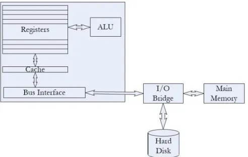
Computers have traditionally had single core processors cast on a CPU chip. The core is comprised of a single set of registers with a corresponding Arithmetic Logic Unit (ALU). Input-output to this unit is done using the bus interface. Other than the main memory, which is accessible using the memory bus, the CPU chip also makes use of available on-chip cache apart from the registers for storing temporary data. This memory hierarchy, consisting of the registers, different levels of cache, and the main memory determines the performance of the CPU while executing data intensive applications by reducing the latency introduced due to accessing of data from main memory or even the external disk drives. The architecture of such a device is shown in Fig. 2.1.

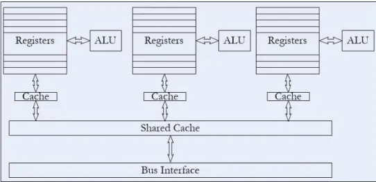
In case of multicore CPUs, the chip consists of multiple sets of ALUs and registers. Each set of an ALU and registers is defined as a core for the computer. Fig. 2.2 shows a chip consisting of 3 cores.

(24)

Figure 2.2: Architecture of a multi-core CPU

computations. CUDA, acronym for Compute Unified Device Architecture, developed by NVIDIA Corporation, provides a programming and memory model for GPUs to help those perform as general purpose graphics processing units (GPGPUs). In the CPU-GPU heterogeneous environment, the GPU is referred to as the “device” and the CPU to which it is connected is called the “host”. The GPU can be controlled and accessed by programs executing on the CPU and data can be transferred to the memory of the device to delegate specific tasks to be performed on it. Earlier, GPUs were specifically used to solve programs that belonged to the graphics domain. One way to utilize the computation power of the GPUs is to convert general programs into equivalent graphics problem, and then solve those problems instead. But this approach is complicated and there is a lot of conversion overhead involved. CUDA enabled GPUs on the other hand allows users to directly execute programs and solve general problems in the original form. The CUDA API (Application Programming Interface) documents all the details as to how the programs that are executed on the CPU can transfer or delegate a part of the program to be executed on the GPU.

CUDA provides a large number of threads that can be executed simultaneously on the cores of the device. To be able to maximize the utilization of the available hardware, it is necessary to have parallel versions of the problems that are expected

(25)

Figure 2.3: Architecture of a GPU (C1060)

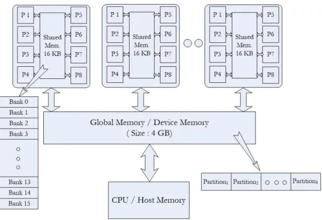
to have performance gain by solving on multicore architecture. Therefore, develop-ing parallel versions of both basic and advanced algorithms for different domains is relevant. Significant performance gains can be achieved by executing highly multi-threaded applications on the CUDA enabled GPUs. But, along with this opportunity to achieve significant speedup, there is the challenge of minimizing the latency intro-duced due to simultaneous data access from the memory. As in CPUs, there is a hierarchy of memory units for the GPUs. Similar to the registers, L1, L2 and other levels of cache which are used to hide the latency introduced by the memory accesses, the GPUs have their own registers and shared memory, which are on-chip and can be used by the GPU for fast execution. The architecture of a GPU is shown in Fig. 2.3. The GPU consists of a number of Streaming Multiprocessors (SMs, 30 for C1060), each containing 8 cores, and have access to the on-chip shared memory of that specific SM. All the cores in all the SMs also have access to the device or global

(26)

memory. The shared memory is further subdivided intobanks and the global memory into partitions. Memory access from different banks and partitions can be done in parallel.

2.3 CUDA

Compute Unified Device Architecture or CUDA is a programming environment for using GPUs to solve general purpose problems. The CUDA environment consists of the CUDA programming model and the CUDA memory model. The programming model for CUDA extends the C programming language and defines C-like functions, called kernels, which are executed in parallel by different CUDA threads. In the following sub-sections we look into the details of CUDA.

2.3.1 CUDA Programming Model

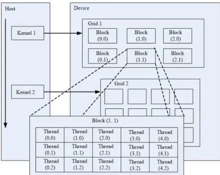
The CUDA programming model provides the basics of how the multi-threaded archi-tecture is designed and functions. The threads are grouped together in blocks, which can be either one, two or three dimensional, and each thread within a block is iden-tified by its unique threadID. All the blocks of threads, identified by blockID, form a one or two dimensional grid. Threads within a block can co-operate among them-selves by accessing data through shared memory and synchronizing their execution to coordinate memory accesses. Blocks of threads are assigned to the multiprocessors by the CUDA scheduler.

The sequential parts of the code is executed on the “host” i.e., the CPU, and the parallel parts are executed on the “device” i.e., the GPU. Blocks of threads execute the kernels. Threads are further divided into execution units called Warps. Each Warp consists of 32 active threads. But for the execution purpose, the scheduler assigns half-warps to the streaming multiprocessors. Therefore, at any instant of time, there

(27)

Figure 2.4: CUDA Programming Model (NVIDIA Corporation, 2010)

are 16 active threads on any multiprocessor. So, the total number of threads in a block are divided and grouped together as Warps, which in turn are further sub-divided into half-warps. The blocks of threads in turn are grouped together to form the Grid, which can be either one or two dimensional as shown in Fig. 2.4.

Threads from different blocks synchronize among themselves by using the Global memory. The maximum number of threads that can reside on a streaming multipro-cessor is limited by the hardware resources. There are a limited number of registers with each of the streaming multiprocessors, and with the increase in their usage, the number of threads decreases. The scheduler assigns more than one block of threads to the same multiprocessor if the total number of threads in the blocks combined is less than what can be handled in each of the multiprocessors.

Parallel programming models are classified primarily based on problem decompo-sition and process interaction. Classification according to problem decompodecompo-sition can be categorized with respect to task parallelism or data parallelism. CUDA follows the SPMD (Single Program Multiple Data) model, which is similar to the SIMD (Single

(28)

Instruction Multiple Data) model. Threads within the same block execute in SIMD fashion, whereas threads of different blocks can execute different portions of the code i.e., the instruction can be different while considering all the streaming multiproces-sors, but the program is the same. This is also referred to as SIMT (Single Instruction Multiple Thread) in many cases.

Considering the process interaction, parallel programming models are broadly classified into Shared Memory Model and Distributed Memory Model. In case of Shared Memory Model, the architecture consists of processors accessing a common or shared memory; the PRAM (Parallel Random Access Machine) model is one such example. There are various versions of the PRAM model, the EREW (Exclusive Read Exclusive Write), CREW (Concurrent Read Exclusive Write) and the CRCW (Concurrent Read Concurrent Write), based on memory read and write patterns. In case of the Distributed Memory Model, the architecture consists of a number of processors each with their own local memory, and interaction among the processors are performed by sending messages. Message Passing Interface or MPI is one such example.

The CUDA programming model is actually a combination of both the Shared and Distributed models. CUDA follows the Shared Memory model if the data is stored and accessed using only the global memory. In this case it follows the EREW model. Message Passing Interface is available for GPU clusters using CUDA-Aware MPI thus making is possible to classify it as Distributed memory model.

2.3.2 CUDA Memory Model

There are different levels in the memory hierarchy of the GPUs. Fig. 2.5 shows the different levels of the memory hierarchy available on a GPU. Table 2.1 summarizes some properties of the levels of memory. Data is transferred from the CPU to the GPU and back using memory copy functions. Global memory is predominantly used

(29)

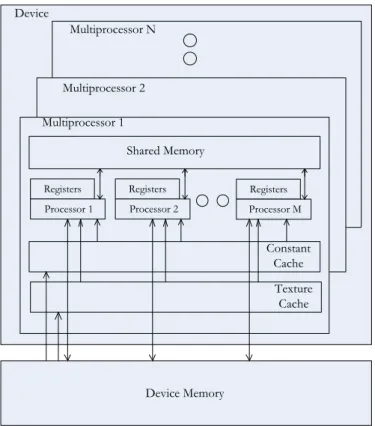
Device Multiprocessor N Multiprocessor 2 Multiprocessor 1 Shared Memory Device Memory Registers Processor 1 Registers Processor 2 Registers Processor M Constant Cache Texture Cache

Figure 2.5: GPU memory hierarchy (NVIDIA Corporation, 2010)

to transfer data from the host to device and vice-versa. In the following section we discuss about different characteristics and usage of the memory model.

Memory Location Access Scope Lifetime

Register On-chip R/W One thread Thread

Local Off-chip R/W One thread Thread

Shared On-chip R/W All threads in a block Block Global Off-chip R/W All threads + host Application Constant Off-chip R All threads + host Application Texture Off-chip R All threads + host Application

(30)

2.4 Memory Hierarchy, Access Patterns and Optimization

Techniques

Memory on the GPU is divided into many different levels. The memory hierarchy of the GPU consists of device memory, shared memory, constant memory, texture memory and registers. The size of each of the above mentioned types of memory varies according to the system, and a comparison of the global and shared memory size for different GPUs is given in Table 2.2. The shared memory is further divided into 16 or 32 banks depending on the system. The global memory is the largest and also has the highest access latency. The on-chip shared memory has significantly faster access compared to the global memory. But, when data is accessed from the same bank, either the same element or different elements in the same bank, then there is a bank conflict leading to a performance loss (the only exception being the case where all the threads access the same element leading to a broadcast.) The constant memory and the texture memory are also located off-chip like the the global memory, but both are read-only memory and data stored in them cannot be modified.

Model CUDA Global Shared # of Memory

# cores Memory Memory Banks

C1060 240 4 GB 16 KB 16

C2050 448 3 GB 48 KB 32

C2070 448 6 GB 48 KB 32

Table 2.2: Architecture Comparison of Different Nvidia GPUs (NVIDIA Corporation, 2010)

Various methods of memory optimization and parallelism management to improve performance of GPUs have been studied (Yang et al., 2010a). The two main consid-erations for efficient processing on the GPUs is to effectively distribute the workload among the threads and also efficiently utilize the memory hierarchy. Identification of

(31)

inefficient workload division or memory accesses in kernels, and reorganizing the code to optimize the memory accesses and maximizing the parallelism using a compiler has been proposed (Yang et al., 2010a). Techniques to improve the performance of the GPUs and performance prediction model has also been studied (Hasan et al., 2014). The focus of the memory optimization techniques can be divided into the following four categories:

To be able to efficiently access data from global memory and utilize the off-chip memory bandwidth, data item might be vectorized and memory coalescing can be taken advantage of.

The shared memory has low access latency, and its optimal usage can be ensured by avoiding bank conflicts.

Workload must be divided among threads in a balanced manner, so that threads scheduled on each of the available multiprocessors does similar amount of work. Data accessed from off-chip global memory must avoid partition camping, which

is similar to bank conflicts, but with much higher performance penalty.

The above mentioned performance issues are applicable to many-core architectures other than the GPUs. These are universal methodologies, and primitives focusing on high memory bandwidth and balanced workload are relevant to a wide range of architectures.

2.4.1 Shared Memory Vs. Global Memory

As evident from the CUDA programming guide (NVIDIA Corporation, 2010) and related work (Boyer et al., 2008), the shared memory is a lot faster than the global memory. So, for all algorithms, whenever it is possible, the data is stored, accessed and modified from the shared memory. As the shared memory has a capacity of 16

(32)

KB (C1060), and different streaming multiprocessors can have different data stored in each of them, the total size of data being processed is limited by that available on the 30 streaming multiprocessors. Therefore, for the C1060 card, the total shared memory available is 480 KB. Although, it must be observed that the entire shared memory might not be available for data storage during the execution of a kernel because of the storage of the kernel parameters and other intrinsic values in it.

2.4.2 Shared Memory Bank Conflicts

The shared memory is of size 16 KB (or 48 KB), and is divided into 16 banks (or 32 banks). Data is stored in consecutive banks, and the width of each bank is 4 bytes.

Figure 2.6: Shared Memory Bank Access: (a) No Conflicts, (b) 8-Way Conflict, (c)Broadcast (NVIDIA Corporation, 2010)

(33)

Now, all the active threads scheduled on the same streaming multiprocessor can access data from any bank on the shared memory. Data access from different banks take place in parallel. If more than one thread accesses data from the same bank,bank conflict occurs, and the accesses become sequential and the memory access latency increases. Fig. 2.6 (a) & (b) shows threads accessing shared memory with no bank conflicts, and also with 8-way bank conflicts. 8-way bank conflicts means 8 threads access data from the same bank at the same time.

In the special case, where all the threads access the same data element from the same bank, the compiler optimizes these memory access operations and issues a broadcast. Therefore, in this case instead of 16-way bank conflict i.e., maximal conflict, there is no conflict at all, and the data is available to all the threads in just a single read operation rather than the required 16 operations. Fig. 2.6 (c) shows threads accessing the same data element in the same bank in the shared memory resulting in the broadcast mechanism taking effect.

But, in the case where even though all the threads access the same bank, but different data elements in the bank, the broadcast mechanism cannot be used. So, maximal bank conflicts occur. The threads are executed on the multiprocessors in groups of 32 referred to as Warps. But, only half of the threads in a warp are active at any instant of time. This can be attributed to the fact that there are 16 banks in the shared memory, and if all the threads in a warp are active, then it is guaranteed to cause at least 2-way bank conflicts. Therefore, by using half-warps, there is a chance that the threads can access the shared memory banks without any conflicts.

2.4.3 Global Memory Access Coalescing

In certain cases, where the size of the data required for computation is larger than that of the shared memory, even when using the most efficient data structures, storing and accessing the data from the global memory is required. Due to the increased latency,

(34)

as evident from the experimental results in (Boyer et al., 2008), the time required to access data from the global memory is much larger than that from the shared memory. Therefore, to reduce the penalty in execution time while using the global memory as the storage for the data, there are certain primitives available for the Nvidia GPUs that can be used. Memory Coalescing is one such mechanism. By taking advantage of memory coalescing, the effects of slower memory accesses can be effectively compensated.

Data from the global memory is accessed in the form of transactions. Therefore, minimizing the number of global memory accesses is equivalent to minimizing the number of transactions.

Let us consider the case where each of the threads in an active half-warp (total 16, identifier idx 0 - 15) accesses elements from an array stored in the global memory using a loop. Also, because of the offset, let the elements accessed by the above mentioned threads are all in separate segments. Therefore, in this case, each step of the loop would require 16 transactions (one for each thread), as shown in Fig. 2.7.

Segment1 Segment2 Segmenti

Global Memory

E1 E2 Ei

Thread1 Thread2 Threadi

Figure 2.7: Global Memory Access: Maximum Transactions

As mentioned earlier, since transactions are expensive as the time required to access data from the global memory is significant, the number of transactions required to get the data for the threads from the global memory can be reduced by using memory coalescing.

(35)

The global memory access by 16 threads (half-warp) is coalesced into a single memory transaction if data accessed by all threads lie in the same segment. Consid-ering the previous example, if the value of offset is modified to a value such that all the data elements accessed by the threads belong to the same data segment, then the number of transactions for each step of the loop reduces from 16 to 1, as shown in Fig. 2.8.

Segment1 Segment2 Segmenti

Global Memory

E1

T1 T2 Ti

E2 Ei

Figure 2.8: Memory Coalescing in Effect: Minimum Transactions

It must be noted that while data elements might be contiguous, they need not be in the same segment. For example, there might be a single transaction required to access 64-bytes of data if it is stored entirely in a single segment. But, for another set of data, accessing a set of 50-bytes might require two transactions if the data is split over two segments in the global memory.

The number of transactions required to access data from the global memory using memory coalescing depends on a number of factors like the compute capability of the system in question and whether the data that is being accessed by the different threads within the active warp is aligned and sequential or non-sequential (NVIDIA Corporation, 2010). A comparison for the different available options is shown in Table 2.3.

From the data available in Table 2.3, it is evident that for CUDA compute ca-pability versions 1.2 and later, accessing non-sequential data is handled in the same

(36)

Compute Access Data Size Memory Capability Pattern in Bytes Transactions

1.0 Sequential 128 2 1.1 Sequential 128 2 1.2 Sequential 128 2 1.3 Sequential 128 2 2.0 Sequential 128 1 1.0 Non-sequential 128 32 1.1 Non-sequential 128 32 1.2 Non-sequential 128 2 1.3 Non-sequential 128 2 2.0 Non-sequential 128 1

Table 2.3: Number of Memory Transactions on different GPUs (NVIDIA Corporation, 2010)

manner as sequential data.

2.4.4 Partition Camping

Although memory coalescing is an efficient technique that can be used to offset the slower access to the global memory, there are other factors that can dictate the actual performance benefit achieved. Partition camping is one such mechanism that dom-inates the outcome of various measures undertaken to access data from the global memory efficiently. Although the shared memory has low access latency, the lim-iting factor is shared memory bank conflicts. Similarly, from the global memory perspective, memory coalescing is the performance booster while the limiting factor is partition camping. Memory coalescing and partition camping deal with data trans-fers between the global and on-chip memories, while bank conflicts deal with on-chip shared memory.

The shared memory on the Nvidia systems is divided into 16 (or 32) banks of 32-bit width. Similarly, the global memory is divided into 6 (or 8) partitions on

(37)

8-and 9-series GPUs (or 200- 8-and 10-series GPUs) of 256-byte width, as shown in Fig. 2.9. Partition1 (256 bytes) Partition2 Partitioni (256 bytes) (256 bytes) Global Memory

Figure 2.9: Global memory divided into partitions

As evident from the previous discussion, for efficient use of the shared memory, bank conflicts must be avoided. This is ensured by distributing the data accessed by the threads in a half warp into the maximum possible available banks. Therefore, the total time to access the data from the shared memory is indirectly proportional to the number of banks accessed by the threads in the active half-warp, and is given in the form of the following equation

β X i=1 Ti ∝ De Pβ i=1Bi (2.1)

where,Ti is the time required for threadi,Deis the number of data elements accessed by the threads, and Pβ

i=1Bi is the total number of distinct banks accessed by all

the threads for computation on the data. Since the Warp-size is 32 and half-warp is 16, the maximum value of β is 16. In the best-case scenario, when there is no bank conflict, the threads access distinct banks and Pβ

i=1Bi = 16. In the worst-case scenario, when all the threads access the same bank but different elements in it thereby negating the usage of the broadcast primitive available with the compiler, Pβ

i=1Bi = 1.

(38)

di-vided into partitions. For efficient usage of global memory, concurrent accesses by all active warps should be divided evenly amongst partitions. Partition camping occurs when global memory accesses are mapped into a subset of partitions, causing requests to queue up at some partitions while other partitions go unused. While memory coa-lescing concerns global memory accesses within a half warp, partition camping deals with global memory accesses amongst active half warps. Therefore, it is analogous to shared memory bank conflicts, but on a wider scale. As shown in Equation[2.1] for shared memory bank conflicts, the total time to access the data from the global memory is indirectly proportional to the number of partitions accessed by the threads in all the active half-warps, and is given in the form of the following equation

γ X i=1 Tiw ∝ Pγ i=1CMi Pγ i=1P arti (2.2)

where, Tiw is the time required for threads in the active warp Wi, CMi is the to-tal number of coalesced memory access required to access the data elements to be processed by the threads in active warp Wi, and Pγ_i₌₁P arti is the total number of distinct partitions accessed by all the threads in warp Wi for computation on the data, and γ gives the total number of active warps. The objective of accessing the data from the global memory efficiently is toMinimize(Pγ

i=1Tiw), which is equivalent toMaximize(Pγ

i=1P arti).

In Fig. 2.10, partition camping effect is illustrated with an example. Let the streaming multi-processors in the Nvidia system be denoted by SMi, where 1≤ i≤ 30. The active warps are given by Wi, where i is the streaming multiprocessor on which it is being executed. Now, if the data in the global memory is distributed in such a manner, that for a given instance of execution, all the active warps access data from the same partition, in this case P artition1, then partition camping takes place.

(39)

Partition1 Partition2 _Partitioni Global Memory P4 P3 P2 P8 P7 P6 P5 SM1 (W1) P 1 P4 P3 P2 P8 P7 P6 P5 SM2 (W2) P 1 P4 P3 P2 P8 P7 P6 P5 SM30 (W30) P 1 W1 W2 W30

Figure 2.10: Partition Camping in Effect

are not accessed. The active warps accessing a particular partition are shown in a table inside the partition.

Partition1 Partition2 Partitioni

Global Memory P4 P3 P2 P8 P7 P6 P5 SM1 (W1) P 1 P4 P3 P2 P8 P7 P6 P5 SM2 (W2) P 1 P4 P3 P2 P8 P7 P6 P5 SM30 (W30) P 1 W1 W9 W25 W2 W8 W10 W16 W24 W17 W18 W26

(40)

In Fig. 2.11, a case where partition camping is avoided is shown. In this case, all the active warps are distributed evenly amongst the available partitions and the mapping is given by the following equation

P artitioni%p ⇐Wi (2.3)

where, pis the total number of partitions available.

2.5 Summary

In this chapter we discuss about GPU architecture and CUDA. The CUDA program-ming model and memory model are studied and techniques to improve the perfor-mance of the same are discussed. Many different devices exist that are CUDA enabled and there have been changes with the availability of newer versions of the architecture. However, the basic principles of the models remain the same, and the discussions are valid across all the different architectures.

(41)

Chapter 3 Storing graphs on GPUs

3.1 Introduction

For performing computations on the GPUs storing the graph data on the device is essential. Using efficient data structures to store the data helps in making use of the level of memory with the least access latency. In this chapter we study the different methods to store graphs on the GPUs.

3.2 Related work

Using efficient data structures to store graphs for computation on both CPUs and GPUs have been studied extensively. Various modifications of the adjacency matrix and adjacency list data structures are considered.

Katz and Kider (Katz & Kider, 2008) and Buluc et al. (Bulu¸c et al., 2010) proposed storing graphs on the GPU by dividing the adjacency matrix into smaller blocks. The required blocks are loaded in the memory, and after computation, are replaced by the next set of blocks. This representation still uses the adjacency matrix, and might include data which is not required for computations based on locality information.

Frishman and Tal (Frishman & Tal, 2007) propose representing multi-level graphs using 2D arrays of textures. They propose partitioning the graph in a balanced way, by identifying geometrically close nodes and putting them in the same partition. Since the partitions are based on locality information and balanced, it makes use

(42)

of the GPUs data parallel architecture. But partitioning the graph itself is a hard problem.

For sparse matrices, the Compressed Sparse Row (CSR) representation is useful (Garland, 2008). Also, representing the edge information using arrays to store the out-vertex and in-vertex numbers saves space for sparse matrices (Itokawa et al., 2007). This method is better suited for directed graphs.

Bader and Madduri (Bader & Madduri, 2008) proposed a technique where different representations are used depending on the degree of the vertices. This is relevant for storing graphs that exhibit the small-world network property, where vertices have an unbalanced degree distribution, with majority of vertices having small degrees and a few vertices are of very high degree.

Harish and Narayanan (Harish & Narayanan, 2007) describe the use of a compact adjacency list, where instead of using several lists, the data is stored in a single list. Using pointers for each of the vertices’ adjacency information, data for the entire graph is kept in a single one dimensional array, which can be significantly large to be stored in the shared memory, and has been implemented in the global memory in their paper.

In this chapter, in addition to using the breadth-first search (BFS) information to carefully split the graph for processing, we introduce data structures for storing nodes and their adjacency information that are in contiguous levels of the BFS-tree. We propose both simple and modified data structures using least number of bits in addition to exploiting the symmetric property of undirected graphs. The modified data structure is similar to the one proposed by Harish and Narayanan (Harish & Narayanan, 2007), but with improvements, including the use of fewer bits in the general case and also using more than one array to store the entire adjacency data for the graph, thereby adhering to stricter memory requirement constraints.

(43)

3.3 Simple data structures for storing the graph information

Various data structures can be chosen to store the adjacency information of graphs in the GPU memory. Each of the different data structures have different storage requirements. There are several operations on graphs that need to access the stored data using one of the available data structures. A memory efficient data structure might have worse time complexity when it comes to accessing the required data for computations. Hence, there exists a trade-off between memory requirement and access time complexity, when choosing the appropriate data structure for storing the adjacency information of the graphs. In this section, we analyze the space required by different data structures and also the time complexity for performing common operations on graphs using the same. It must be noted that throughout the chapter, for calculations we use boolean data and it consists of a single bit, and does not refer to the data type available in programming languages.

3.3.1 Adjacency Matrix

For a graph G= (V, E) with |V|=n, the size of adjacency matrix is n2 bits, where each edge is stored using a single bit. To fit the adjacency matrix in the shared memory, the space required must be less than or equal to that of the desired level in the memory hierarchy of the GPU. Considering the architecture available on the Nvidia 10-series GPUs, for example C1060, the size of the shared memory is 16 KB. Hence, to satisfy the above constraint, n2 _≤ _131,_{072 (16 KB = 16}_×₁₀₂₄_×₈

bits = 131,072 bits), which gives n ≈ 360. Therefore, using the adjacency matrix representation, the size of the largest graph that can be kept in the shared memory is 360 (assuming all shared memories in the different streaming multiprocessors contain identical data.)

(44)

3.3.2 Upper Triangular Matrix

The adjacency matrix representation contains redundant information, and those can be eliminated to reduce the storage requirements. For undirected graphs, values (i, j) and (j, i) are identical. So, storing only the Upper Triangular Matrix (UTM) of the adjacency matrix is enough, which requires n×(n₂+1) bits. So, the largest graph that can be kept in the shared memory using the UTM representation is 511. As all the values of (i, i) = 0, using the Strictly UTM representation (S-UTM) (i.e. without the data on the diagonal), size of the largest graph that can be kept in the shared memory is 512. Although the shared memory spans across 16 banks, it is preferable to store data for any specific node within a single bank thereby avoiding potential memory contention and reduce overall execution time. With the above requirement, the number of nodes that can fit in the shared memory is reduced to 506, where data is kept in increasing order of the node numbers. Also, using UTM representation, the number of nodes’ data in each of the bank (size 8192 bits) varies, as shown in Table 3.1.

In the previous approach due to unbalanced distribution of nodes, threads assigned to operate on banks with more nodes would have to do significantly more work than the threads accessing banks with less number of nodes. On the other hand, if threads access a constant number of nodes it will result in inefficient memory utilization, thus limiting the overall size of graph that can be stored.

For load balancing the distribution can be done as follows. Using S-UTM rep-resentation different rows have different amount of data (see Table 3.2). To make the structure rectangular (see Table 3.3), the space gained by not storing redundant information in any row in the upper part of the S-UTM can be filled up by a corre-sponding row from the lower part. When n is even, the space gained in rowi is filled with data values from row n − i (see Table 3.3); when n is odd, the corresponding

(45)

Bank Nodes in the # of Nodes Space Required # Bank in bits 0 0-15 16 7976 1 16-31 16 7720 2 32-48 17 7922 3 49-66 18 8073 4 67-85 19 8170 5 86-104 19 7809 6 105-124 20 7830 7 125-146 22 8151 8 147-169 23 8004 9 170-194 25 8100 10 195-221 27 8046 11 222-251 30 8085 12 252-285 34 8075 13 286-325 40 8020 14 326-378 53 8162 15 379-505 127 8128

Table 3.1: Distribution of nodes in the banks

space in row i is filled with data from rown −(i+ 1) (see Table 3.5). In general, for any value of n the number of rows of data is reduced from n to n₂. This is called Balanced S-UTM (B-S-UTM), where all rows have the same amount of data, each corresponding to that of 2 nodes. The above method is similar to “rectangular full packed” in dense linear algebra (Gustavson et al., 2010). With the desire to store an entire row of data in a single streaming multiprocessor, this scheme also ensures all banks have equal number of nodes in them thereby achieving load-balancing. Us-ing this scheme, the maximum number of rows that can be kept in a sUs-ingle bank is

(1024×8)

511 ≈16. As there are 2 nodes’ data in each row, the total number of nodes’ data

(46)

this manner in the 16 banks is 32×16 = 512. – a b c d e f g – – h i j k l m – – – n o p q r – – – – s t u v – – – – – w x y – – – – – – z φ – – – – – – – ψ – – – – – – – –

Table 3.2: S-UTM for even number of nodes

a b c d e f g

h i j k l m ψ

n o p q r z φ

s t u v w x y

Table 3.3: S-UTM with load balanced approach for even number of nodes

– a b c d e f – – g h i j k – – – l m n o – – – – p q r – – – – – s t – – – – – – u – – – – – – –

Table 3.4: S-UTM for odd number of nodes

a b c d e f u

g h i j k s t

l m n o p q r

(47)

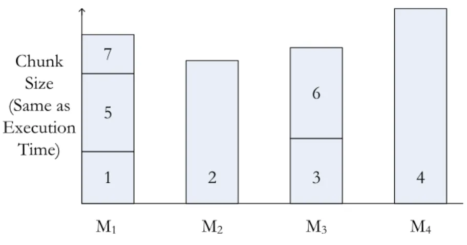
The number of simultaneous thread executions is limited by the number of GPU processors in a streaming multiprocessor. Each thread is allocated a set of combina-tions of nodes (with cardinalityk) and a thread is to determine if the desired property (e.g., do they form a connected subgraph?) holds. In order to use all available GPU processors in other streaming multiprocessors, we have to duplicate the graph and place it on all the shared memories on other streaming multiprocessors. Care must be taken to ensure each thread is given a unique set of combinations to test, to avoid duplication in work.

The sets of combination ofk nodes are allocated to each streaming multiprocessor as follows. Since the shared memory in each streaming multiprocessor can store up to 512 nodes, it can be assumed that there are 512 sets of combinations, each start-ing with a unique node number. We allow the first 29 streamstart-ing multiprocessors to operate on 17 unique sets of combinations each and the last streaming multiprocessor operates on the remaining 19 sets (17×29 + 19 = 512). In each streaming multipro-cessor, depending on the number of threads the unique sets are uniformly divided to be processed.

3.3.3 Adjacency List Using Array of Linked Lists

Other than the adjacency matrix, adjacency list is also a common data structure used to store graph information. There can be various modifications in the implementation of the adjacency list, and each has different memory requirements and data access complexity. In this sub-section, we study the implementation of the adjacency list using an array of linked lists, also referred to in here as AL-AL, and is shown in Fig. 3.1.

Let the total number of nodes in the graph be nand total number of edges be m. Here, all the nodes are stored in an array; the identifiers of the nodes given by the indices of the array location. Each array element contains a pointer to the starting

(48)

0 1 ₂ 5 3 4 6 1 2 0 1 2 6 0 2 3 0 1 3 4 5 3 4

64 bits logn bits _{64 bits}

An example graph (left) with the corresponding adjacency list representation (right) using Array of Linked Lists (AL-AL)

X X

X

Figure 3.1: Adjacency List Using Array of Linked Lists

node of the linked list representing the neighbors of the corresponding node i.e., the edge information. In the example graph shown in Fig. 3.1, node 0 is connected to nodes 1 and 2. Therefore, a pointer to node 1 is stored in the array index corre-sponding to node 0. The storage for node 1 contains the identifier for the node, and a pointer to the next neighbor i.e., node 2. Since, there are no more neighbors for node 0, the pointer associated with node 2 contains an invalid marker, denoted in Fig. 3.1 by “X”. Now, each of the edges would be stored two times, once for each end vertex. Considering a 64-bit machine, each of the pointers require 64 bits. So, the space needed to store the array containing the nodes is given by n×64 bits. Now, each of the edges are represented by the end vertex number, and also contains a pointer to the next edge information if there exists another edge for the node under consideration. Since there aren nodes in the graph, representing a node number requires logn bits. Hence, for storing each of the edges, the space required is (logn+ 64) bits, giving a total of 2m×(logn+ 64) bits for all the edges. Therefore, the total size required for this representation is given by n×64 + 2m×(logn+ 64) bits.

(49)

3.3.4 Adjacency List Using Array of Arrays

In the adjacency list representation using array of linked lists, there are too many pointers involved in the implementation, thereby increasing the size of the data struc-ture. Using arrays to group data together replacing pointers can reduce the memory required, and this is referred to as adjacency list using array of arrays, and is shown in Fig. 3.2. log n bits 0 1 ₂ 5 3 4 6 1 3 0 2 4 Array Pointer (64 bits) 0 1 2 2 # of neighbors (log n bits)

An example graph (left) with the corresponding adjacency list representation (right) using Array of Arrays (AL-AA)

6

3 3

2

Figure 3.2: Adjacency List Using Array of Arrays

Here the edges from each node are stored using arrays instead of linked list. Since there are no pointers involved between edges, to determine the size of the array, the number of neighbors for each of the nodes need to be stored. In this case, all the nodes in the graph are stored in an array, along with the number of neighbors and in addition there is a pointer for each of the nodes to the array containing its neighbors. In the example graph shown in Fig. 3.2, node 1 is connected to 3 nodes, numbered 0, 2 and 3. Therefore, for node 1, a value of 3 is stored corresponding to the number of neighbors, and also a pointer to the array of its neighbors, which contains

(50)

the identifiers for the nodes 0, 2 and 3. The size of the array with the number of neighbors and pointers for the n nodes require n ×(logn+ 64) bits. Additionally, the total space required for all the arrays containing information about the m edges is 2m×logn bits. Therefore, the total size required for this representation in bits is given by n×(logn+ 64) + 2m×logn.

An improved version of this data structure that requires less storage is one which does not store the number of neighbors for each of the nodes. However, this in-formation is required to retrieve the adjacency data, and must be available during computation. This can be achieved by using the sizeof() function on the array con-taining the neighbors to find the required number at runtime. Hence, the array of arrays variant with the sizeof() function requires n×64 + 2m×logn bits.

3.3.5 Adjacency List Using Array Implementation of Linked Lists

In the adjacency list representation using array of arrays, there are still pointers involved, and that requires significant amount of space. Instead of using pointers, the information for the edges can be stored using an array and relevant identifiers. So, the linked list pointers are replaced by using arrays. This representation is referred to as the adjacency list using array implementation of linked lists, and is shown in Fig. 3.3.

Here, both the nodes and edges are stored in arrays. Each element for the node array contains the starting index position in the array containing the edges. Since there are 2m indices in the edge array, the values stored in the node array each require log 2m bits, giving a size of n×log 2mbits for the node array. The edges are represented by a pair of elements in the edge array. The first element contains the end vertex number of the edge, and the second element contains the index position of the next edge information in the array, or an identifier value of “-1” which indicates the end of the linked list. As there are n nodes, the first element requires logn bits,

(51)

An example graph (left) with the corresponding adjacency list representation (right) using Array Implementation of Linked List (AL-ALL)

0 1

n-1 4

Start index position of the array linked list that

contains the edges

0 2m-1 1 2 3 4 1 2 2 -1 End of linked list 0 18 19 40 10 ... ... ... ... 10 2 0 3 -1 0 1 ₂ 5 3 4 6

Figure 3.3: Adjacency List Using Array Implementation of Linked Lists and for the 2m indices possible, the second element requires log 2m bits. So, the size of the edge array is 2m×(logn+ log 2m) bits. Therefore, the total size required for this representation in bits is given by n×log 2m+ 2m×(logn+ log 2m).

Now, the data representing the edges can be stored in any order in the array implementing the linked list. In the example graph shown in Fig. 3.3, the neighbors of node 0 are stored starting at position 4 in the array just to illustrate the fact that data can be stored at any location in the array as the pointers would correctly determine the location of the next available data. Node 1, which is a neighbor of node 0 is stored at location 4, and contains a pointer to location 2. Location 2 contains the identifier of the other neighbor of node 0 i.e., node 2 and contains an identifier “-1” for the pointer indicating the end of the list since there are no more neighbors