1
POWER QUALITY ESTIMATION AND
CLASSIFICATION USING WAVELETS
Bachelor of Technology
in Electrical Engineering
Department of Electrical Engineering
National Institute of Technology, Rourkela
MAY 2014
Under supervision of
PROF SANJEEB MOHANTY
Submitted by
DEEPAK KUMAR EKKA
(110EE0194)
2
POWER QUALITY ESTIMATION AND
CLASSIFICATION USING WAVELETS
A Thesis submitted in partial fulfillment of the requirements for the degree of
Bachelor of Technology
in “
Electrical Engineering
”
By
DEEPAK KUMAR EKKA
110EE0194
UNDER THE GUIDANCE OF
Prof. Sanjeeeb Mohanty
Department of Electrical Engineering
National Institute of Technology
3
DEPARTMENT OF ELECTRICAL ENGINEERING
NATIONAL INSTITUTE OF TECHNOLOGY,
ROURKELA
ODISHA, INDIA-769008
CERTIFICATE
This is to certify that the Thesis report entitled “
POWER QUALITY
DETECTION AND CLASSIFICATION USING WAVELETS
”,
submitted to the National Institute of Technology, Rourkela by
Mr.
Deepak Ku.Ekka
, Roll No: 110EE0194 for the award of Bachelor of
Technology in Electrical Engineering is a bona- fide record of
research work carried out by him under my supervision and guidance.
The candidate has fulfilled all the prescribed requirements. The draft
report which is based on candidate’s own work has not been
submitted elsewhere for a degree/diploma. In my opinion, the draft
report is of standard required for the award of a Bachelor of
Technology in Electrical Engineering.
Prof. Sanjeeb Mohanty
Supervisor
Department of Electrical Engineering
4
ACKNOWLEDGEMENTS
I would like to express my sincere gratitude to my supervisor
Prof. Sanjeeb Mohanty
for his guidance, encouragement, and
support throughout the term of this work. It was an indispensable
learning experience for me to be one of his students. As my
supervisor hisinsight, observations and suggestions helped me to
establish the overall direction of theresearch and contributed
immensely for the success of this work.
My thanks are extended to my colleagues in power control and drives,
who built anacademic and friendly research environment that made
my study at NIT, Rourkela mostfruitful.
DEEPAK KUMAR EKKA
110EE0194
5
TABLE OF CONTENTS
PAGECERTIFICATE 03
ACKNOWLEDGEMENT 04
TABLE OF CONTENTS 05
DEFINATIONS OF DIFFERENT POWER QUALITY EVENT05
ABSTRACT 08
LIST OF TABLES 09
LIST OF FIGURES 09
LIST OF ABBRIEVIATION 10
1.
Chapter I INTRODUCTION 12
1.1 Main objective of the project 12
1.2 Basic layout of the project 13
2.
Chapter II Application of wavelet transform 14
2.1 Discrete Wavelet Transform (DWT) 14
2.2 Generation of the PQ Signals in MATLAB 18
2.3 Detection using DWT 19
3.
Chapter III De-noising of PQ events 25
3.1 Steps involved in de-noising 25
3.2 Thresh-holding rule 25
3.3 Result of de-noising 26
4.
Chapter IV Feature extraction 30
4.1 Introduction 30
4.2 Feature Extraction Vectors 30
4.3 PQ Database 31
5.
Chapter V Classification and Conclusion 38
5.1 Flow Diagram for classification 39
5.2Conclusion 40
6
DEFINATIONS OF DIFFERENT POWER QUALITY DISTURBANCES
As defined by the
IEEE
the various disturbed signals are:
SAG
: It may be defined as the sudden drop of the voltage magnitude from its
nominal value typically lasting from a cycle to a second or so, or tens of
milliseconds to hundreds of milliseconds.
SWELL
: sudden rise of voltage magnitude from its nominal value typically
lasting from a cycle to a second or so, or tens of milliseconds to hundreds of
milliseconds.
INTERRUPTION
: sudden drop of the voltage magnitude from its nominal
value to negligible or very less magnitude. It can be momentary, temporary or
long term.
SURGE
: Sudden rise of voltage magnitude for a very short period.
HARMONICS
: It is the sinusoidal component of a periodic wave or quantity
having a frequency that is integer multiple of fundamental frequency.
7
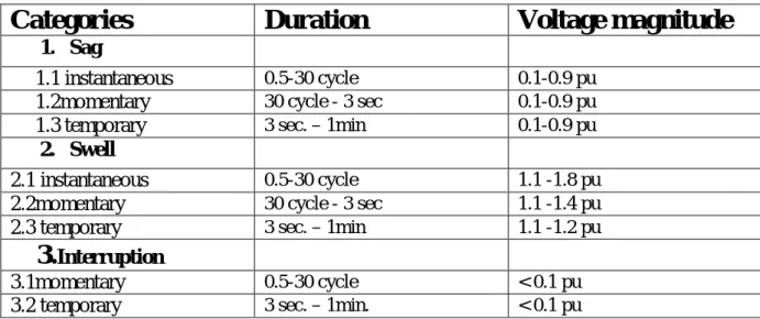
TABLE.1FOR PQ FOR SHORT DURATION INTERVALS
Categories
Duration
Voltage magnitude
1. Sag
1.1 instantaneous 0.5-30 cycle 0.1-0.9 pu
1.2momentary 30 cycle - 3 sec 0.1-0.9 pu
1.3 temporary 3 sec. – 1min 0.1-0.9 pu
2. Swell
2.1 instantaneous 0.5-30 cycle 1.1 -1.8 pu
2.2momentary 30 cycle - 3 sec 1.1 -1.4 pu
2.3 temporary 3 sec. – 1min 1.1 -1.2 pu
3.
Interruption3.1momentary 0.5-30 cycle < 0.1 pu
3.2 temporary 3 sec. – 1min. < 0.1 pu
TABLE OF PQ FOR LONG DURATION INTERVAL
Categories
Duration
Voltage magnitude
1.Long Durationvariation 1.1 Interruption >1 min. 0.0 pu 1.2Under-voltage >1 min. 0.8-0.9 pu 1.3 Over-voltage >1 min. 1.1-1.2 pu 2.Transient 2.1 Impulsive(millisecond) >1m sec 0-4 pu 2.2Oscillatory 0.3-50 m sec.
8
ABSTRACT
Due to increase in the number of electric and electronic equipment along with the fast controlling power electronic devices, which has affected the main power quality events(PQ).These are namely short-circuits , notching, voltage sag and swell, harmonics and transient due to load switching. Whenever these disturbances occur, these last for few cycles and simple observation of waveforms in the bus-bar will not help to recognise the problem in there and henceforth will not be able to identify and sort out the problem. If such events occur for few more cycles/minute it may result to overvoltage and under-voltage, or long time power interruption or any other problem.
Hence, an approach is developed for the detection and location of time and finally classifies the different power quality events including both the transients and steady state signals. By using one of the signal processing we can decompose namely wavelet decomposition by using “DISCRETE WAVELET TRANSFORM (DWT)”.In a sampling frequency, we can samples those signals and any change on the smoothness is detected at finer resolution levels of decomposition. By the decomposition process we get the power coefficients or wavelet packets which are necessary performance indices of the signal. We are in generally using the
a) THD (Total Harmonic Distortion) and
b) Energy of the signal to classify them in the PQ event analysis.
The main purpose of the paper also focuses on using the MATLAB WAVELET TOOL GUIDE, for the study of De-noising and other purpose.
Also we have to understand the mathematical tools used in the discrete wavelet transform (DWT) starting from the decomposition algorithm to the de-noising as well as thresh-holding of the PQ signals which are necessary in monitoring the classification scheme.
9
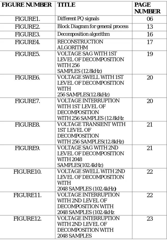
LIST OF FIGURES
FIGURE NUMBER TITLE
PAGE
NUMBER
FIGURE1.
Different PQ signals
06
FIGURE2.
Block Diagram for general process
13
FIGURE3.
Decomposition algorithm
16
FIGURE4.
RECONSTRUCTION
ALGORITHM
17
FIGURE5.
VOLTAGE SAG WITH 1ST
LEVEL OF DECOMPOSITION
WITH 256
SAMPLES (12.8kHz)
19
FIGURE6.
VOLTAGE SWELL WITH 1ST
LEVEL OF DECOMPOSITION
WITH
256 SAMPLES(12.8kHz)
20
FIGURE7.
VOLTAGE INTERRUPTION
WITH 1ST LEVEL OF
DECOMPOSITION
WITH 256 SAMPLES (12.8kHz
20
FIGURE8.
VOLTAGE TRANSIENT WITH
1ST LEVEL OF
DECOMPOSITION
WITH 256 SAMPLES(12.8kHz)
21
FIGURE9.
VOLTAGE SAG WITH 2ND
LEVEL OF DECOMPOSITION
WITH 2048
SAMPLES(102.4kHz)
21
FIGURE10.
VOLTAGE SWELL WITH 2ND
LEVEL OF DECOMPOSITION
WITH
2048 SAMPLES (102.4kHz
)
22
FIGURE11.
VOLTAGE INTERRUPTION
WITH 2ND LEVEL OF
DECOMPOSITION WITH
2048 SAMPLES (102.4kHz
22
FIGURE12.
VOLTAGE INTERRUPTION
WITH 2ND LEVEL OF
DECOMPOSITION WITH
2048 SAMPLES
10
FIGURE13.
VOLTAGE TRANSIENT WITH
2ND LEVEL OF
DECOMPOSITION
WITH 2048 SAMPLES
23
FIGURE14.
VOLTAGE SAG ALONG WITH
THIRD ORDER WITH 2ND
LEVEL
OF DECOMPOSITION WITH
2048 SAMPLES (102.4kHz)
24
FIGURE15.
VOLTAGE SAG ALONG WITH
THIRD AND FIFTH ORDER
WITH
2ND LEVEL OF
DECOMPOSITION WITH 2048
SAMPLES (102.4kHz)
24
FIGURE16.
DE-NOISED VOLTAGE SWELL
SIGNAL
23
FIGURE17.
DE-NOISED VOLTAGE SWELL
SIGNAL
23
FIGURE18.
DE-NOISED VOLTAGE
TRANSIENT SIGNAL
27
FIGURE19.
DE-NOISED VOLTAGE
INTERRUPTION
SIGNALSIGNAL
27
FIGURE20.
DE-NOISED VOLTAGE SAG
WITH THIRD HARMONIC
SIGNAL
28
FIGURE22.
CLASSIFICATION
FLOWCHART
39
LIST OF TABLES
TABLE
NUMBER
TITLE
PAGE
NUMBER
Table1.
Different PQ signal for long and short
duration
07
Table2.
GENERATION OF THE PQ
DISTUBANCES
18
Table3.
TRANSIENT AND INTERRUPTION
THD AND ENERGY
32
11
ENERGY
Table5.
VOLTAGE SAG WITH THIRD
HARMONICS THD AND ENERGY
34
Table6.
VOLTAGE SAGWITH THIRD AND
FIFTH HARMONICS THD AND
ENERGY
35
Table7.
VOLTAGE SWELL THD AND
ENERGY
36
Table8.
VOLTAGE SWELL THD WITH
THIRD HARMONICS AND
ENERGY
37
Table9.
VOLTAGE SWELL THD WITH
THIRD AND FIFTH HARMONICS
AND ENERGY
38
LIST OF ABBREVIATIONS
PQ –
POWER QUALITY
DWT-
DISCRETE WAVELET TRANSFORM
FT-
FOURIER TRANSFORM
STFT-
SHORT TIME FOURIER TRANSFORM
FFT-
FAST FOURIER TRANSFORM
THD-
TOTAL HARMONIC DISTORTION
SNR-
SIGNAL TO NOISE RATION
12
Chapter I INTRODUCTION
As discussed earlier that now-a-days due to power electronic equipments and its increasing use in the industry, the power quality (PQ) getdetoriated. Most of the equipments are sensitive to thevariations in power quality. Some of the problems associated with the poor quality are malfunctioning, short lifetime, power interruption, over voltages and under voltages. Therefore it has become a dire need to monitor and detect the disturbances as well classify them in an intelligent manner. Comparing with the other signal processing processes like Fourier Transform (FT), Short time Fourier Transform (STFT) and Fast Fourier Transform, which makes an analysis just in spectral analysis ad is applied to steady state conditions not in the transients as well as at high frequency.The Discrete Wavelet Transform (|DWT) on the other handis preferred for its window for sampling in the time frequency variations results better in time frequency response.
1.1
MAIN OBJECTIVE OF THE PROJECT :
The main purpose of the project is to develop a signal processing method i.e. Discrete wavelet transform (DWT).It should be able to detect the different power quality events and finally classifying these signals using a classifier based on the feature extraction of the PQ signal.
13
Generation of the Decomposition of the De-noising of the PQ
PQ signals PQ signals and detection signals
Classification on Feature-
Energy and THD Extraction
Figure 2.Block diagram for the general process
1.2 BASIC LAYOUT OF THE PROJECT
As shown in the figure.2 the various processes which we are required to carry out the wavelet analysis of the PQ signals which are basically as follows:
1. To generate the power quality signals along with disturbances. 2. To undergo wavelet decomposition as well as reconstruction. 3. To de-noise the PQ signals with noise.
4. Feature extraction of performance index using the coefficients of the wavelets. 5. Finally classifying them based on the basis of THD and Energy of the signal.
14
CHAPTER I focuses on the need of PQ detection and monitoring scheme for the classification purpose. It also compares the DWT procedures with other signal processing methods.
CHAPTER II focuses on explaining the DWT signal processing methodology. It starts with the definitions and the methods which are required to extract the necessary coefficients namely approximate and detail coefficients. It also tries to recognise the signals in different frequencies of sampling. Also the problem associated with noise in case of detection is discussed.
CHAPTER III focuses on the de-noising of the signal parameters along with the performance indices like Signal-to-Noise Ratio (SNR) and Mean Square Error (MSE).
CHAPTER IV focuses on the performance indices of the signals. By obtaining the coefficients in wavelet decomposition procedure, we can obtain the THD and Energy of the different PQ signal, which are having different sets of values.
CHAPTER V focuses on classifying them within the threshold limit and by certain parameters. Finally a flow diagram to classify the power signals is made.
Chapter II Application of DWT
2.1 DISCRETE WAVELET TRANSFORM
DWT is a strong mathematical and analytical computing method in signal processing which carries out the transformation of the PQ events. In other words, DWT develops a windowed frame of certain samples taken in the value which can be modulated by signal cutting problem. The only idea of the scheme is to looking different resolutions and time-frequency
15
domain for both steady-state and transients unlike the Fourier Transform (FT). In this paper, we are going to generate different PQ signals and decomposing them in different levels by the DWT and the change in the smoothness of the signal is detected at different resolutions. I t is quite evident that PQ disturbances has the unique deviation from the pure sinusoidal waveform and thus reliable to classify them based on energy concept.
The basic step in the signal processing of the DWT involves two stages which are as follows: 1. Determining the wavelet coefficients
2. Reconstruction of the signal by these coefficients
In brief, the first stage includes determining the wavelet coefficients ℎ ( ) and ( ). These coefficients transform them from the time domain to wavelet domain. After the completion of the first stage, these coefficients are approximated and detailed version of the pure signal. The transformation formula is as shown below:
=
∑
( ).
(
−
+
)
………(2.1)
=
∑
( ).
(
−
+
)
………(2.2)
Now this process is repeated to obtain the level 2 decomposition and hence all the coefficients on wavelet domain are found out from the time domain by the reconstruction procedure.
16 FIGURE 3.DECOMPOSITION ALGORITHM
FIGURE 3 BASIC DECOMPOSITION ALGORITHMS
The wavelet transform of the signal is given by
( , ) =
∫
∞( )
∗
, ( )
∞
………(2.3)
Where ( , ) ℎ of the signal ( ) and
, ( ) =( )
√ is scaled and shifted from the mother wavelet(t). The parameter ‘a’ is the scale
and time domain property is ‘b’.
√ is the normalization value of a,b(t). Here band pass filter is
assumed as it has both high pass and low pass characteristics. The low pass filter
17
approximates the signal wheras the high pass filter provides the detail lost in the approximation
FIGURE 4.RECONSTRUCTION ALGORITHM
Here in the block diagram for the reconstruction algorithmℎ reprsents the low pass filter and repersents the high pass filter which approximates and details during reconstruction algorithm.
Choice of Mother Wavelets
The choice of filter coefficients is very necessary as if not chosen correctly there will be detection problem. As we know there are two types of disturbances: slow transients and fast transients. The waveforms in the fast transients have rapid changes and sharp edges where Daub4 and Daub6 gives better results then the other coefficients due to less time and compactness. In general, Daub8 and Daub10 coefficients are use in slow changes and transients. F(n) 2 2 2 2 2 2
18
2.2 GENERATION OF THE PQ DISTUBANCES
TABLE 2 GENERATION OF DIFFERENT PQ SIGNALSTYPE OF PQ
DISTURBANCE
S
MODEL EQUATION
VARIATION
Voltage sag v=(1-A*(u(t-t1)-u(t-t2))).*sin(2*pi*50*t); A=(0.1-0.9) and t1-t2=(0.2-0.4 seconds)
Voltage swell v=(1+A*(u(t-t1)-u(t-t2))).*sin(2*pi*50*t); A=(0.1-0.9) and t1-t2=(0.2-0.4 seconds)
Voltage interruption v=(1-(u(t)-u(t-t1)+u(t-0.4))).*sin(2*pi*50*t); A=0 and t1-t2=(0.2-0.4 seconds)
Voltage transient v=(1+A*(u(t-t1)-u(t-t2))).*sin(2*pi*50*t); A=2-3 and t1-t2=(0.21-0.22 seconds) Voltage Sag with
third Harmonics v=(1-A*(u(t-t1)-u(t-t2))).*(sin(2*pi*50*t)+(0.333*(sin(2*pi*50*3*t) ))); A=(0.1-0.9) and t1-t2=(0.2-0.4 seconds) Voltage Swell with
third harmonic v=(1+A*(u(t-t1)-u(t-t2))).*(sin(2*pi*50*t)+(0.333*(sin(2*pi*50*3*t) ))); A=(0.1-0.9) and t1-t2=(0.2-0.4 seconds)
The various types of PQ events were generated using MATLAB code using the above equations namely, voltage sag, voltage swell, transients and interruption with harmonic contents.
SPECIFICATION OF THE SIGNALS
Frequency of the signal = 50 Hz Frequency of sampling = 102.4 kHz No. of samples = 2048 no. of samples. Total time of signal = 0.5 seconds.
19
2.3 DETECTION USING DWT
From MATLAB codes we have generated the different power quality signal disturbances at the frequency of 50 Hz with a sampling rate of 102.4kHz with 2048 number of samples along with the impact of the disturbances is0.2 seconds to 0.4 seconds. As we know that for more number of decomposition levels we have to decompose with higher sampling frequencies. The accuracy of the detection is dependent on the level of decomposition. So, we have to also compare those signals with two different sampling frequencies namely 102.4 and12.8 kHz.
FIGURE5. VOLTAGE SAG WITH 1ST LEVEL OF DECOMPOSITION WITH 256 SAMPLES (12.8kHz)
The voltage signal is generated and by Daub 8, the slow changing power quality events have been decomposed in level 1decomposition of wavelet transform. The approximate and detail coefficients are also obtained only in case of transients the Daub 4 is used. But for further
0 0.05 0.1 0.15 0.2 0.25 0.3 0.35 0.4 0.45 0.5 -1 0 1 PQ SIGNAL 0 50 100 150 200 250 300 -2 0 2
LEVEL 1 DECOMPOSITION SIGNAL
0 20 40 60 80 100 120 140 -2 0 2 APPROXIMATE SIGNAL 0 20 40 60 80 100 120 140 -0.2 0 0.2 DETAILED SIGNAL
20
level of decomposition we have to sample those at higher frequency levels namely at 102.4 kHz with 2048 no of samples. 0 0.05 0.1 0.15 0.2 0.25 0.3 0.35 0.4 0.45 0.5 -2 0 2 PQ SIGNAL 0 50 100 150 200 250 300 -5 0 5
LEVEL 1 DECOMPOSITION SIGNAL
0 20 40 60 80 100 120 140 -5 0 5 APPROXIMATE SIGNAL 0 20 40 60 80 100 120 140 -0.2 0 0.2 DETAILED SIGNAL
21
FIGURE6. VOLTAGE SWELL WITH 1ST LEVEL OF DECOMPOSITION WITH 256 SAMPLES(12.8kHz)
FIGURE7. VOLTAGE INTERRUPTION WITH 1ST LEVEL OF DECOMPOSITION WITH 256 SAMPLES (12.8kHz)
FIGURE8. VOLTAGE TRANSIENT WITH 1ST LEVEL OF DECOMPOSITION
0 0.05 0.1 0.15 0.2 0.25 0.3 0.35 0.4 0.45 0.5 -1 0 1 PQ SIGNAL 0 50 100 150 200 250 300 -2 0 2
LEVEL 1 DECOMPOSITION SIGNAL
0 20 40 60 80 100 120 140 -2 0 2 APPROXIMATE SIGNAL 0 20 40 60 80 100 120 140 -0.2 0 0.2 DETAILED SIGNAL 0 0.05 0.1 0.15 0.2 0.25 0.3 0.35 0.4 0.45 0.5 -5 0 5 PQ SIGNAL 0 50 100 150 200 250 300 -2 0 2
LEVEL 1 DECOMPOSITION SIGNAL
0 20 40 60 80 100 120 140 -2 0 2 APPROXIMATE SIGNAL 0 20 40 60 80 100 120 140 -1 0 1 DETAILED SIGNAL
22
FIGURE9. VOLTAGE SAG WITH 2ND LEVEL OF DECOMPOSITION
FIGURE10.VOLTAGE SWELL WITH 2ND LEVEL OF DECOMPOSITION 0 0.05 0.1 0.15 0.2 0.25 0.3 0.35 0.4 0.45 0.5 -1 0 1 PQ SIGNAL 0 500 1000 1500 2000 2500 -2 0 2
LEVEL 2 DECOMPOSITION SIGNAL
0 200 400 600 800 1000 1200 -2 0 2 APPROXIMATE SIGNAL 0 200 400 600 800 1000 1200 -0.02 0 0.02 DETAILED SIGNAL 0 0.05 0.1 0.15 0.2 0.25 0.3 0.35 0.4 0.45 0.5 -2 0 2 PQ SIGNAL 0 500 1000 1500 2000 2500 -5 0 5
LEVEL 2 DECOMPOSITION SIGNAL
0 200 400 600 800 1000 1200 -5 0 5 APPROXIMATE SIGNAL 0 200 400 600 800 1000 1200 -0.02 0 0.02 DETAILED SIGNAL
23
FIGURE11 .VOLTAGEINTERRUPTION WITH 2ND LEVEL OF DECOMPOSITION 0 0.05 0.1 0.15 0.2 0.25 0.3 0.35 0.4 0.45 0.5 -1 0 1 PQ SIGNAL 0 500 1000 1500 2000 2500 -2 0 2
LEVEL 2 DECOMPOSITION SIGNAL
0 200 400 600 800 1000 1200 -2 0 2 APPROXIMATE SIGNAL 0 200 400 600 800 1000 1200 -0.02 0 0.02 DETAILED SIGNAL 0 0.05 0.1 0.15 0.2 0.25 0.3 0.35 0.4 0.45 0.5 -1 0 1 PQ SIGNAL 0 500 1000 1500 2000 2500 -2 0 2
LEVEL 2 DECOMPOSITION SIGNAL
0 200 400 600 800 1000 1200 -2 0 2 APPROXIMATE SIGNAL 0 200 400 600 800 1000 1200 -0.05 0 0.05 DETAILED SIGNAL
24
FIGURE12.VOLTAGE INTERRUPTION WITH 2ND LEVEL OF DECOMPOSITION
FIGURE13. VOLTAGE TRANSIENT WITH 2ND LEVEL OF DECOMPOSITION
Similarly we can obtain the third level of decomposition.The third decomposition level of only the sag with third and fourth order armonics signal is as shown.
FIGURE14. VOLTAGE SAG ALONG WITH THIRD ORDER WITH 2ND LEVEL OF DECOMPOSITION 0 0.05 0.1 0.15 0.2 0.25 0.3 0.35 0.4 0.45 0.5 -1 0 1 PQ SIGNAL 0 500 1000 1500 2000 2500 -2 0 2
LEVEL 2 DECOMPOSITION SIGNAL
0 200 400 600 800 1000 1200 -2 0 2 APPROXIMATE SIGNAL 0 200 400 600 800 1000 1200 -0.2 0 0.2 DETAILED SIGNAL 0 0.05 0.1 0.15 0.2 0.25 0.3 0.35 0.4 0.45 0.5 -1 0 1 PQ SIGNAL 0 500 1000 1500 2000 2500 -5 0 5
LEVEL 3 DECOMPOSITION SIGNAL
0 200 400 600 800 1000 1200 -2 0 2 APPROXIMATE SIGNAL 0 200 400 600 800 1000 1200 -0.05 0 0.05 DETAILED SIGNAL
25
FIGURE15. VOLTAGE SAG ALONG WITH THIRD AND FIFTH ORDER WITH 2ND LEVEL OF DECOMPOSITION
Chapter III De-noising of PQ events
The main problem in the detection part of the PQ disturbances is noise. Most of the signals classification is greatly degraded in distinguishing the power quality distuerbances and noise. Hence before the classification of the signal, the signal must be de-noised. One of the application of the wavelet analysis is the de-noising by certain methods.
3.1 Steps involved in de-noising the signal
In general to DWT it involves the above two steps discussed in chapter II and one more thresh-holding. The three steps which are involved in de-noising are as follows:
0 0.05 0.1 0.15 0.2 0.25 0.3 0.35 0.4 0.45 0.5 -1 0 1 PQ SIGNAL 0 500 1000 1500 2000 2500 -5 0 5
LEVEL 3 DECOMPOSITION SIGNAL
0 200 400 600 800 1000 1200 -2 0 2 APPROXIMATE SIGNAL 0 200 400 600 800 1000 1200 -0.1 0 0.1 DETAILED SIGNAL
26
1. Decomposition: As usual we have to select the mother wavelet as “db4” or Daub4 as they are compact. It is for high frequency and fast transients which means sharp changes. The level of decomposition is also selected which is 5 in this case.
2. Detail coefficient thresh-holding: For the detail coefficients a soft threholding method in MATLAB is chosen.
3. Reconstruction: Similar to the wavelet analysis, the reconstruction of the signal is the same to the reconstruction algorithm of Discrete Wavelet Transform (DWT)
3.2 Thresh-holding rule
Here all the signals are added with a Gaussian noise to add them as noise, the noisy signal is then decomposed into db4 or Daub4 by level 5 decoposition scheme. The noise signal is then decomposed by DWT to the same level to generate wavelet coefficients which are
approximate and detail coefficients. Let S(n) be the noise signals with the PQ signal F(n).
( ) = ( )+∈. ( )………(3.1)
Where n=0,1,2..k-1 and e(n) corresponds to noise signal. In MATLAB the common denoising they are:-
1. “rigrsure” 2. “heursure” 3. “sqtwolog” 4. “minimax”
'rigrsure' : It uses the soft threshold estimator. It is a a threshold selection rule based on the Stein's Unbiased Estimate of Risk (quadratic loss function).
'sqtwolog' It uses a fixed form threshold yielding ‘minimax’ performance multiplied by a small factor proportional to log(length(s)).
27
‘heursure' is a mixture of the two previous options. As a result, if the signal-to-noise ratio is very small, the SURE estimate is very noisy. So if such a situation is detected, the fixed form threshold is used.
'minimaxi' uses a fixed threshold chosen to yield minimax performance for mean square error against an ideal procedure.
3.3 Results of de-noising
As white Gauss noise is added to the signal and then the signal is de-noised using the thresh-holding schemes as discussed earlier. Now the different types of signals are denised using the above methods and the results are as shown in the figures:-
FIGURE16. DE-NOISED VOLTAGE SWELL SIGNAL
200 400 600 800 1000 1200 1400 1600 1800 2000
-5 0 5
Noisy signal - Signal to noise ratio = 3
200 400 600 800 1000 1200 1400 1600 1800 2000
-5 0 5
De-noised signal - heuristic SURE
200 400 600 800 1000 1200 1400 1600 1800 2000
-5 0 5
De-noised signal - SURE
200 400 600 800 1000 1200 1400 1600 1800 2000
-5 0 5
De-noised signal - Fixed form threshold
200 400 600 800 1000 1200 1400 1600 1800 2000
-5 0 5
28
FIGURE17.DE-NOISED VOLTAGE SWELL SIGNAL
20 40 60 80 100 120 140 160 180 200
-1 0 1
Noisy signal - Signal to noise ratio = 3
20 40 60 80 100 120 140 160 180 200
-1 0 1
De-noised signal - heuristic SURE
20 40 60 80 100 120 140 160 180 200
-1 0 1
De-noised signal - SURE
20 40 60 80 100 120 140 160 180 200
-1 0 1
De-noised signal - Fixed form threshold
20 40 60 80 100 120 140 160 180 200
-1 0 1
29
FIGURE18 DE-NOISED VOLTAGE TRANSIENT SIGNAL
FIGURE19 DE-NOISED VOLTAGE INTERRUPTION SIGNALSIGNAL 200 400 600 800 1000 1200 1400 1600 1800 2000 -5
0 5
Noisy signal - Signal to noise ratio = 3
200 400 600 800 1000 1200 1400 1600 1800 2000 -5
0 5
De-noised signal - heuristic SURE
200 400 600 800 1000 1200 1400 1600 1800 2000 -5
0 5
De-noised signal - SURE
200 400 600 800 1000 1200 1400 1600 1800 2000 -5
0 5
De-noised signal - Fixed form threshold
200 400 600 800 1000 1200 1400 1600 1800 2000 -5
0 5
De-noised signal - Minimax
50 100 150 200 250 300
-1 0 1
Noisy signal - Signal to noise ratio = 3
50 100 150 200 250 300
-1 0 1
De-noised signal - heuristic SURE
50 100 150 200 250 300
-1 0 1
De-noised signal - SURE
50 100 150 200 250 300
-1 0 1
De-noised signal - Fixed form threshold
50 100 150 200 250 300
-1 0 1
30
Similarly for the transients and for the harmonic content level the de-noised signals are plotted
FIGURE20 DE-NOISED VOLTAGE SAG WITH THIRD HARMONIC SIGNAL
FIGURE21.DE-NOISED VOLTAGE SAG WITH THIRD AND FIFTH HARMONIC SIGNAL
100 200 300 400 500 600 700 800 -1
0 1
Noisy signal - Signal to noise ratio = 3
100 200 300 400 500 600 700 800 -1
0 1
De-noised signal - heuristic SURE
100 200 300 400 500 600 700 800 -1
0 1
De-noised signal - SURE
100 200 300 400 500 600 700 800 -1
0 1
De-noised signal - Fixed form threshold
100 200 300 400 500 600 700 800 -1
0 1
De-noised signal - Minimax
200 400 600 800 1000 1200 1400 1600 1800 2000 -5
0 5
Noisy signal - Signal to noise ratio = 3
200 400 600 800 1000 1200 1400 1600 1800 2000 -5
0 5
De-noised signal - heuristic SURE
200 400 600 800 1000 1200 1400 1600 1800 2000 -5
0 5
De-noised signal - SURE
200 400 600 800 1000 1200 1400 1600 1800 2000 -5
0 5
De-noised signal - Fixed form threshold
200 400 600 800 1000 1200 1400 1600 1800 2000 -5
0 5
31 CONCLUSION
Hence, after getting the result from this chapter it is quite evident that the DWT
transformation helps a lot in de-noising of the signal. The thresh-holding technique is qutite efficient in de-niosing the signls from noise and most of them are cleared. After this the signals are sent for feature extraction using the basic perfomance indices like THD and Energy of the signal. The presence of the noise will have greatly affected in the classification of all the signals in PQ detection and classification.
Chapter IV Feature Extraction
4.1
Introduction
For the design of the monitoring scheme for the detection of the PQ disturbance signals the prime necessity is the extraction of the above de-noised signal. The feature extraction is quite important in designing the monitoring system. For that we have to have a database based on certain performance indices which will be in help to distinguish the PQ signals with less ambiguity and redundancy. The basic performance indices of the system are THD and Energy of the signal which will classify these signals into different PQ events.
4.2
Feature Extraction Vector
As discussed earlier the two parameters which help in classifying the above signals are THD and Energy of the signal. Another benefit in using the DWT transform theory is that we can easily get these two parameters using the coefficients of DWT.
32 THD (Total Harmonic Distortion)
In each frequency ranges, the distortion harmonics which are included can be detected by using the approximation and detail coefficient which are in turn obtained by Discrete Wavelet Transform (DWT).
In terms of RMS values
=
∑
(
( ) )
……….4.1
Where N(j) is the number of detail coefficient at scale j. Hence, by these coefficients THD can be calculated as follows
=
∑ ( )
∑ ( )
……….4.2
Energy of the signal
Similarly, Energy of the signal is calculated as follows:
=
∫
( )
=
∑
( )
+
∑
∑
( )
………...4.3
Where C(k)j and D(k)j are the approximate and detail coefficients respectively in the wavelet decomposition procedure.
4.3
PQ Database
As we have generated the various signals in MATLAB and then by Discrete Wavelet Transform decomposed into coefficients which are in turn used as for calculating the parameters of THD and Energy spectrum of the signal. Now for further we have de-noised the signal using the de-noising of the MATLAB and DWT functions which are fed
33
input to the extraction of signal parameters namely THD and energy. So we have to make a database such that we can classify them in their PQ events without any ambiguity.
At first the signal with less parameter variations are tabulated as
below:
TABLE3. TRANSIENT AND INTERRUPTION THD AND ENERGY
Type of PQ
disturbance
THD magnitude
Energy in(volt^2 -
second)
Transient
0.6342
1.0214*
34
VOLTAGE SAG
The voltage sag signal is maintained with disturbance time of (0.2-0.4) seconds. After that the disturbance level is varied from 0.1 to 0.9
V = (1-A*(u(t-t1)-u(t-t2))).*sin(2*pi*50*t);………..………...4.4
Finally after de-noising and decomposition the following table is obtained as follows:
TABLE4. VOLTAGE SAG THD AND ENERGY
MAGNITUDE OF
DISTURBANCE(%)
THD
ENERGY(volt^2 –sec)
10
0.525
0.946*
10
20
.05205
0.876*
10
30
0.5195
0.815*
10
40
0.5200
0.761*
10
50
0.5205
0.716*
10
60
0.5211
0.679*
10
70
0.5217
0.651*
10
80
0.5225
0.630*
10
90
0.5234
0.618*
10
Hence, the threshold levels for the THD and for the energy signals are: 1. THD :0.5195 to 0.5250
35
VOLTAGE SAG WITH THIRD HARMONIC
TABLE5. VOLTAGE SAG WITH THIRD HARMONICS THD AND ENERGY
MAGNITUDE OF
DISTURBANCE(%)
THD
ENERGY(volt^2 –sec)
10
0.5362
0.131*
10
20
0.5360
0.121*
10
30
0.5359
0.113*
10
40
0.5358
0.105*
10
50
0.5357
0.099*
10
60
0.5356
0.094*
10
70
0.5355
0.0903*
10
80
0.5354
0.087*
10
90
0.5352
0.085*
10
The voltage sag signal is maintained with disturbance time of (0.2-0.4) seconds. After that the disturbance level is varied from 0.1 to 0.9
V=(1-A*(u(t-t1)-u(t-t2))).*(sin(2*pi*50*t)+(0.333*(sin(2*pi*50*3*t)))...(4.5)
Hence, the threshold levels for the THD and for the energy signals are:
1. THD :0.5352 to 0.5362 2. ENERGY: (0.085 to 0.131)*10
36
VOLTAGE SAG WITH THIRDAND FIFTH HARMONIC
TABLE6. VOLTAGE SAGWITH THIRD AND FIFTH HARMONICS THD AND ENERGY
MAGNITUDE OF
DISTURBANCE(%)
THD
ENERGY(volt^2 –sec)
10
0.54541
1.089*
10
20
0.54564
1.0886*
10
30
0.54584
0.938*
10
40
0.54562
0.876*
10
50
0.54565
0.824*
10
60
0.54578
0.782*
10
70
0.54572
0.749*
10
80
0.54575
0.725*
10
90
0.54598
0.711*
10
The voltage sag signal is maintained with disturbance time of (0.2-0.4) seconds. After that the disturbance level is varied from 0.1 to 0.9
V =(1-A*(u(t-t1)-u(t-t2))).*(sin(2*pi*50*t)+
(0.333*(sin(2*pi*50*3*t)))+(0.2*(sin(2*pi*50*5*t))))
………..4.6
Hence, the threshold levels for the THD and for the energy signals are:
1.
THD : 0.54551 to 0.54598
37
VOLTAGE SWELL
TABLE7. VOLTAGE SWELL THD AND ENERGY
MAGNITUDE OF
DISTURBANCE(%)
THD
ENERGY(volt^2 –sec)
110
0.53323
1.0889*
10
120
0.53414
1.0850*
10
130
0.53512
1.0654*
10
140
0.53617
1.0589*
10
150
0.53721
1.0515*
10
160
0.53769
1.0423*
10
170
0.53775
1.0398*
10
180
0.53819
1.0129*
10
190
0.53897
1.0091*
10
The voltage sag signal is maintained with disturbance time of (0.2-0.4) seconds. After that the disturbance level is varied from 0.1 to 0.9
V=(1+A*(u(t-t1)-u(t-t2))).*sin(2*pi*50*t);…….4.7
Hence, the threshold levels for the THD and for the energy signals are: 1. THD :0.53323 to 0.53897
38
VOLTAGE SWELL WITH THIRD HARMONICS
TABLE8. VOLTAGE SWELL THD WITH THIRD HARMONICS AND ENERGY
MAGNITUDE OF
DISTURBANCE(%)
THD
ENERGY(volt^2 –sec)
110
0.5548
1.23120*
10
120
0.5549
1.33780*
10
130
0.55434
1.45150*
10
140
0.55384
1.57440*
10
150
0.55338
1.70630*
10
160
0.55294
1.84740*
10
170
0.55252
1.99750*
10
180
0.55214
2.15680*
10
190
0.55178
2.32520*
10
The voltage sag signal is maintained with disturbance time of (0.2-0.4) seconds. After that the disturbance level is varied from 0.1 to 0.9
V=(1-A*(u(t-t1)-u(t-t2))).
*(sin(2*pi*50*t)+(0.333*(sin(2*pi*50*3*t))));………...4.8
Hence, the threshold levels for the THD and for the energy signals are as per the database are 1. THD : 0.55178 to 0.5548
39
VOLTAGE SWELL WITH THIRD AND FIFTH HARMONICS
TABLE9. VOLTAGE SWELL THD WITH THIRD AND FIFTH HARMONICS AND ENERGY
MAGNITUDE OF
DISTURBANCE(%)
THD
ENERGY(volt^2 –sec)
110
0.54501
1.2775*
10
120
0.54483
1.3850*
10
130
0.54467
1.5030*
10
140
0.54451
1.6311*
10
150
0.54437
1.7680*
10
160
0.54423
1.9139*
10
170
0.54410
2.0690*
10
180
0.54394
2.2345*
10
190
0.54387
2.4084*
10
The voltage sag signal is maintained with disturbance time of (0.2-0.4) seconds. After that the disturbance level is varied from 0.1 to 0.9
V =(1+A*(u(t-t1)-u(t-t2))).
*(sin(2*pi*50*t)+(0.333*(sin(2*pi*50*3*t)))+(0.2*(sin(2*pi*50*5*t))))………..4.9
Hence, the threshold levels for the THD and for the energy signals are:
1.
THD : 0.54387 to 0.54501
2.
ENERGY
: (1.2 to 2.4)∗10Chapter V Classification and Conclusion
40
NO YES
YES NO YES NO
FIGURE.22 CLASSIFICATION FLOWCHART
Conclusion
Generated PQ signals 1. Wavelet decomposition 2. De-noising 3. Feature extraction THD and ENERGY calculated IS THD> 0.6 IS Energy> 1.01 IS Energy> 1.01 SWELL SIGNAL SAG SIGNAL TRANSIENT SIGNAL INTERRUPTION SIGNAL41
In this part of the work different PQ disturbances with different fault magnitude are generated and the feature vector containing Energy and THD are extracted based on the equation (4.2) and equations as discussed in section 4.2 and a database is prepared. It is observed that the value of THD and Energy is increased considerably if the PQ disturbance contains harmonics. By looking in the database of the PQ disturbance signals, it is quite convenient that different PQ signals are associated with different sets of THD and Energy for example the voltage interruption signal has the lowest energy whereas the Swell signal has the highest energy. For taking the corrective measures in the power system, there is a need of correctly detecting and estimating the PQ disturbances in a processed manner .For the study here we have taken nearly six types of signals including harmonics and noise along with sag and swell signals. The first step includes finding the coefficients of decomposition by DWT and reconstruction algorithm. The WT is an approach in frequency domain where the signals are analysed at different frequency resolution levels. The only problem in the detection is that the noise level, if present in the signal then signal classification is much more difficult. Therefore, we have to de-noise the signals again by using DWT different methods of functions. After de-noising of the signals we have to extract the feature vectors like THD and energy of each signals and then classifying them into their different PQ events by selecting some threshold values. Finally a flow cart have been prepared to show different classifications in Figure.22
42
References
1. Quinquis,“Digital Signal Processing using Matlab,”,ISTE WILEY, pp.279-305, 2008. 2. S.Pait,”Detection and classification of PQ using wavelet transform”,IEEE annual
conference 2010. 3. S. Tuntisak,” Harmonic Detection in Distribution SystemUsing Wavelet
Transform”, IEEE Conference on Power Tech 2007. 4. S. Santoso,” “Power Quality Disturbances Classification Using Wavelet ”IEEE
Transactions on Power Delivery April 1996. 5. R. Polikar, ”The Engineer’s Ultimate Guide to Wavelet analysis”,
The Wavelet Tutorial. March 1999. 6. M.Bollen,”Time Frequency and Time Scale Domain Analysis of Voltage
Disturbances,”IEEE Transactions on Power Delivery, October 2000. 7. S.Santoso,”Characterization of distribution power quality events with fourier and