Algorithms for inverse big data problems

(1)

Algorithms for inverse big data problems

Serge Gratton University of Toulouse

CERFACS-IRIT

Joint work with E. Bergou, S. Gurol, E. Simon, D. Titley-Peloquin, Ph.L. Toint, J. Tshimanga,L.N. Vicente, Z. Zhang

(2)

A dynamical system is characterized by state variables, e.g. velocity components pressure density temperature gravitational potential

Goal: predict the state of the system at a future time from

dynamical integration model observational data

Applications: climate, meteorology, oceanography, neutronics, finance, ...

(3)

A dynamical integration modelpredicts the state of the system given the state at an earlier time.

! integrating may lead to very largeprediction errors

! (inexact physics, discretization errors, approximated parameters)

Observational data are used to improve accuracy of the forecasts.

! but the data areinaccurate (measurement noise, under-sampling

! 107 observations (109 variables) processed every day: inverse big

(4)

(5)

data

(6)

−2 −1 0 1 −1

0 1

known situation 2 days ago and background prediction

record data for the past 2 days

minimize the di↵erence between the model and observations

(7)

−2 −1 0 1 −1

0 1

known situation 2 days ago and background prediction record data for the past 2 days

(8)

−2 −1 0 1

−1 0 1

(9)

−2 −1 0 1 −1

0 1

(10)

Notations and toy example Subspace and model reduction Weak contraints Conclusion

Modeling and toy example Dual iterative solvers

Using subspace ideas, subspace reduction

Ensemble methods with a stochastic dynamical system Variational methods with a stochastic dynamical system Summary, caveat and ongoing related work

(11)

Notations and toy example Subspace and model reduction Weak contraints Conclusion

Modeling and toy example

Dual iterative solvers

(12)

A vibrating string

We consider a vibrating string, hold fixed at both ends

It is released with a zero initial speed, from an unknown position The string remains in the vertical plane

The string is observed with a set of physical devices measuring the position string at regularly spaced points during a given time span We would like to

make a forecast of the string position outside the observation time span

Observations1

0 x

u(x)

(13)

A vibrating string : the model

The string positionu(x) is the solution of the partial di↵erential equation 8 < : @2 @t2u(x,t) @ 2 @x2u(x,t) = 0 in ]0,1[⇥]0,T[ u(0,t) =u(1,t) = 0, t 2]0,T[ u(x,0) =u0(x),_@@_tu(x,0) = 0, x 2]0,1[

Under regularity assumptions on u0, this system has one unique

solution

We suppose that the system is observed at timetn,n 0

The problem reads minu0

PNobt

n=0 ku(:,tn) ynk2

This is an infinite dimensional linear least squares problem, that has to

(14)

The observations

We consider now that the string is observed regularly in time and

space. No noise,moreobservations than unkonwns

The discretized version of linear least-squares problem minu0

PNobt

n=0 ku(:,tn) ynk2 is solved with aconjugate gradient

technique

! test(’over’)

(15)

Realistic di

ffi

cult case

In practice, observing a 3D field at all space points is out of reach

! test(’under’)

The observations are noisy, which introduces high frequencies in the analysis

! test(’noisy’)

Both e↵ect (always) come together

(16)

Exploiting ”a priori” information

We do not consider the previous solution acceptable, because we doubt a string might take such positions. We expect the solution to be smooth enough

We would like to introduce the fact that the string position should

not vary too much when considering points that areclose in the

physical space

purely algebraic approach, e.g. minu0 PNobx j=0 1|u0j u0j+1|2+ PNobt n=0 ku(:,tn) ynk2s.t. discretized dynamics

using a pseudo-physical smoothing process

(17)

Smoothing in the discretized space with the heat equation

We consider the discretized heat equation

8 < : @ @tu(x,t) @ 2 @x2u(x,t) = 0 in ]0,1[⇥]0,T[ u(0,t) =u(1,t) = 0, t 2]0,T[ u(x,0) =u0(x), x 2]0,1[

For a given T,u(.,T) is smoother thanu0, because high frequency

(18)

(19)

Solve a large-scale non-linear weighted least-squares problem: min x2Rn 1 2kx xbk 2 B 1 + 1 2 N X j=0 Hj Mj(x) yj 2_R 1 j where

x ⌘x(t0) is the control variable

Mj are model operators: x(tj) =Mj(x(t0))

Hj are observation operators: yj ⇡Hj(x(tj))

the obervations yj and the background xb are noisy

(20)

Back to the realistic di

ffi

cult case

Underdetermined case

! test(’under-reg’)

Noisy case

! test(’noisy-reg’)

Underdetermined and noisy case

(21)

Issues on background regularization

Background matrix mat-vec in CG : another di↵erential equationhas

to be solved

In case of modelling,when a direct solution not applicable, an

inner-outer iteration scheme has to be controlled

Determining a reasonable background matrix : based on physical

considerations, possibly onstatisticsover past assimilation periods

Introduction of balanced relations in the background : when variables

are related to each other by relations that are not accounted for in the model and not properly observed, an additional (weak) penalty term is added

(22)

min x2Rn 1 2kx xbk 2 B 1 + 1 2 N X j=0 Hj Mj(x) yj 2_R 1 j Algorithmic considerations:

very largeproblem size: m⇠107 observations, n⇠108 unknowns

iterative methods for nonlinearproblems:

primal/dual formulations? [S. Gratton and J. Tshimanga (2009) ; S. Gratton, P. Toint, and J. Tshimanga, 2011.]

preconditioning? [S. Gratton, A. Sartenaer, J. Tshimanga, A.T. Weaver (2008) ; S. Gratton, P. Laloyaux, A. Sartenaer, and J. Tshimanga (2001) ]

using of subspace information? handle stochastic dynamical systems?

(23)

Notations and toy example

Subspace and model reduction Weak contraints Conclusion

Modeling and toy example

Dual iterative solvers

(24)

Solve a large-scale non-linear weighted least-squares problem:

min x2Rn 1 2kx xbk 2 B 1 + 1 2 N X j=0 Hj Mj(x) yj 2_R 1 j

Typically solved using a truncated Gauss-Newton algorithm (known as 4D-Var in the DA community)

! linearize Hj Mj(x(k)+ x(k)) ⇡Hj Mj(x(k)) +H_j(k) x(k)

! solve the linearized subproblem

min x(k)₂_Rn 1 2k x (k) ₍_x b x(k))k2_B 1 + 1 2 H (k) _x(k) _d(k) 2 R 1 ! update x(k+1)₌_x(k)₊ _x(k)

(25)

Defining the constraint as "=H x d we can write Lagrangian function

for the quadraticproblem as

L( x,", ) = 1 2kx+ x xbk 2 B 1+ 1 2k"k 2 R 1+ T(" H( x) +d)

From Karush-Kuhn-Tucker conditions, the following stationary conditions are satisfied at any optimum:

r xL( x,", ) =B 1(x+ x xb) HT = 0 r"L( x,", ) =R 1"+ = 0

r L( x,", ) =" H x +d = 0

(26)

Exploiting the structure: Dual Approach

Theexact solution is either

xb xk+BHkT (HkBHkT+R) 1(dk Hk(xb xk))

| {z }

Lagrange mult. : requires solving a linear systemiterativelyinRm

or, from normal equations

xb xk+ (B 1+HkTR 1Hk) 1HkTR 1(dk Hk(xb xk))

| {z }

linear systemiterativelyinRn

Ifm<<n, then performing theminimization inRm_{can both reduce memory and}

computational cost

Nonlinear problem: we want to solve iteratively and truncate afterfew stepsin a

trust-region tuncated CG solver. Does it hurt to use this dual approach?

(27)

Dual/Primal approach compared

Cost function: J( xk) = 1₂k xk xb+xkk2_B 1+ 1₂kHk xk dkk2_R 1

Blue primal - Red dual

the relation between primal and dual formula is lost when an iterative

solver is truncated prematurely

This is bad news for the nonlineariterations

(28)

Preconditioned CG algorithm

For i = 0,1, ...

1 _q_i _{= (}_B 1₊_HT_R 1_H₎_p_i

2 _↵i ₌_<_r_i_,_z_i _{> / <}_q_i_,_p_i _> _{Compute the step-length}

3 _x_i₊₁₌ _x_i₊↵ipi Update the iterate

4 _r_i₊₁₌_r_i _↵i_q_i _{Update the residual}

5 _z_i₊₁₌ _F _r_i₊₁ _{Update the}_{preconditioned residual}

6 _i ₌<ri+1,zi+1> / <ri,zi> Ensure A-conjugate directions

7 _p_i₊₁₌_z_i₊₁₊ _i_p_i _{Update the descent direction}

(29)

Subspace and model reduction Weak contraints Conclusion Initialization steps given v0;r0 = (HTR 1H + B 1)v0 b,. . . Loop: WHILE 1 HTbq_i ₁ = HT(R 1HB 1HT + I_m)bp_i ₁ 2 ↵_i ₁ = rT i 1zi 1/bqiT1bpi 1 3 BHTbv_i = BHT(v_i ₁ + ↵_i ₁bp_i 1) 4 HTbr_i = HT(r_i ₁ + ↵_i ₁qb_i 1) 5 BHTbz_i = FHTbr_i = BHTGbr_i FHT =BHTG 6 _i = (rT i zi/riT1zi 1) 7 BHTbp_i = BHT( bz_i + _ibp_i 1)

(30)

Subspace and model reduction Weak contraints Conclusion Initialization 0= 0,br0=R 1(d H(xb x)), b z0=Gbr0,pb1=bz0,k= 1 Loop on k 1 _b_q_i ₌_Abb_p_i 2 ↵i=<_bri 1,bzi 1>M/ <bqi,bpi >M 3 _i ₌ _i ₁₊_↵i_b_p_i 4 b_r_i ₌b_r_i ₁ ↵ibqi 5 _i₌<_bri 1,bzi 1>M/ < bri 2,bzi 2>M 6 _b_z_i₌_G_b_r_i 7 _b_p_i ₌_b_z_i ₁₊ _i_b_p_i ₁ b A=R 1_HBHT₊_I m G is the preconditioner M is the inner-product RPCGAlgorithm: M=HBHT

preserves monotonic decrease on quadratic cost

Gshould be symmetric w.r.t. toM NeedBHT_G₌_FHT

(31)

Observations: SST (Sea Surface Temperature) and SSH(Sea Surface Height) observations from satellites. Sub-surface hydrographic observations from floats

Number of observations (m): 105

Number of state variables (n): 106_{for strong constraint and 10}7_{for weak constraint}

Computation: 64 CPUs

(32)

Let Fk be s.p.d.. Is the relationFkHkT =BHkTGk reasonable ?

Perfect preconditioner :

(B 1+H_kTR 1Hk) 1HkT =BHkT(HkBHkT+R) 1

IfHkBHkT is nonsingular, andIm(FHkT)⇢Im(BHT), there is always

a unique Gk that corresponds to Fk. But don’t want to compute

Gk = (HkBH_kT +R) 1FkH_kT: too expensive

We focus on quasi-Newton Limited Memory Preconditioner [Morales

and Nocedal 2000] [Gratton, Sartenaer and Tshimanga 2011] that are widely

used in applications

[Gratton, Gurol and Toint 2012] derivethe quasi-Newton LMP in dual

space which generatesmathematically equivalent iterates to those of primal approach

(33)

F

as a Quasi-Newton Limited Memory Preconditioner

Quasi-Newton LMPs are simply based on the idea that generates

preconditioners by using LBFGSupdating formula

Fk+1 = (In ⌧kpkqkT)Fk(In ⌧kqkpkT) +⌧kpkpkT ⌧k = 1/(qkTpk) qk = (B 1+HTR 1H)pk The pairs Fk defined by Fk =Fk+1 Fk, is min Fk W1/2 FkW1/2 F subject to Fk = FkT, Fk+1qk =pk

whereW is a positive definite matrix satisfying Wpk =qk. MatrixF

approximates the inverse of the system matrix: a preconditioner Serge G. Large-scale inverse problems

(34)

G

as a Quasi-Newton Limited Memory Preconditioner

GivingF, we can find G that satisfies FHT ₌_BHT_G

G can be derived by using the formula for F using the relations

pi = BHTbpi,

qi = HTbqi

Gk+1 = (Im b⌧kbpk(Mbqk)T)Gk(Im ⌧bkbqkbpkTM) +b⌧kbpkbpkTM

M =HBHT

b

pk is the search direction

b

qk = (Im+R 1HBHT)bpk The dual pairs

b

⌧k = 1/(bqkTHBHTbpk)

(35)

The quasi-Newton LMP in dual space (Nonlinear case)

In the nonlinear iterations, inheriting the previous preconditioner Gk 1

may not be possible because we need the existence ofFk, s.p.d,

satisfying FkHkT =BHkTGk 1

Theinherited matrixGk 1 may not satisfy HkFkHkT

=HkBHkTGk 1 for anyFk, s.p.d..

The method can be improved by using a safeguarding strategy, whose convergence relies on the Cauchy decrease and a trust-region

”magical” step

(36)

Numerical experiment on heat equation (1/3)

The dynamical model is considered to be the nonlinear heat equation defined by x t 2_x u2 2_x v2 +f[x] = 0 in⌦⇥(0,1) x[u,v,t] = 0 on ⌦⇥(0,₁)

where the temperature variable x[u,v,t] depend on both timet and

position given by spatial coordinates u and v. The functionf[x] is defined by

f[x] =exp[⌘x]

(37)

Numerical experiment on heat equation (2/3)

f[x] =exp[⌘x] ⌘ = 2

(38)

Numerical experiment on heat equation (3/3)

f[x] =exp[⌘x] ⌘= 4.2

(39)

(40)

Subspace and model reduction

Weak contraints Conclusion

Gradient based approach DFO

Nemo, GYRE configuration

Sea level anomaly (top left), velocities (top right), temperature (bottom left) and salinity (bottom right)

North Atlantic circulation with its Gulf stream current.

The basin has 3180 km length, 2120 km width and 4, 5 km depth. State of length 90000

(41)

A subspace from physical considerations

Physical considerations:

The ocean and the atmosphere exhibit anattractor: a slowly varying

geometrical oject that contains the state

Most of the variability can be explained in the “attractor subspace”

(of low dimension r)

! Minimize first in this subspace (of basisL)

(42)

Empirical Orthogonal Functions (EOFs)

Construction of L:

Let x1_{, . . . ,}_xp₂_Rn _{be a set of}_{state vectors}

BuildC = _p1₁Pp_i₌₁(xi _¯_x₎₍_xi _¯_x₎T

Compute theeigenvectors of C (EOFs)

Storer eigenvectorscorresponding to thelargest eigenvalues

! Already used in the reduced Kalman filters(SEEK filter)

(43)

Choice for

r

Selectr such that: Pr i=1 i Pn i=1 i 0.9 ( i &)

!Ther= 100 yields more than 90%

(44)

Using the subspace

[Gratton, Laloyau, Sartenaer, Tshimanga 2011]

The solution of the first system in the subspace spanned byLcan be

obtained with a Ritz-Galerkin formula:

x₀0=xb+L(LTA0L) 1LTb0

It is also possible to approximate the inverse Hessian with aLimited

Memory Preconditioner H =hIn L(LTA0L) 1LTA0 i h In A0L(LTA0L) 1LT i + L(LTA0L) 1LT

We also experimented the use of asmoother (↵t based) on the

vectors in L

Possible to keepA0L from past iteration orrecompute (linearization)

(45)

Subspace solution

(46)

Subspace solution with linearization

(47)

Using the subspace

[Gratton, Laloyau, Sartenaer 2014]

The Ritz-Galerkin starting point corresponds to solving the quadratic

minimisation probleminside the subspace Im(L)

Since this subspace it typically of dimension less then 1000, using derivative free optimization techniques is conceivable, even on the

nonlinear function

Possible scheme, by processing vectors by e.g. batches of 10 members

fork= 1, ..

1 _{Build a new subspace}_L_k

2 _{Minimize function in a}_ffi_{ne space}_x_k₊_Im_L_k _{to get}_x_k₊_L_k_w_K

SID-PSM[Custodio, Vicente 2007], see also [Vaz, Vicente 2009])

3 _Set_x_k₊₁₌_x_k₊_L_k_w_K_r

(48)

Subspace solution

A criterion⇡i to promote subspace vectorsli for whichlarge variationof the cost function

occurs (singular value i) is used:

⇡i=⌧i+ ·

maxj⌧j

maxj j i

,where⌧i =kh(x0) h(x0+li)kR 1

Vectorsli can besmoothed

See[Gratton, Vicente, Zhang 2014]for extension to full domain decomposition and stochastic methods. Also see[Gratton, Royer, Vicente, Zhang 2014]for a complexity analysis ofstochastic direct searchand[Diouane, Gratton, Vicente 2014]for similar algorithms in globally convergent evolution algorithms

(49)

Ensemble methods with a stochastic dynamical system

Variational methods with a stochastic dynamical system Summary, caveat and ongoing related work

(50)

Weak-constraint 4D-Var

min x2Rn 1 2kx0 xbk 2 B 1+ 1 2 N X j=0 Hj xj yj 2_R 1 j +1 2 N X j=1 kxj Mj(xj 1) | {z } qj k2 Q_j 1 x = 0 B B B @ x0 x1 .. . xN 1 C C C A2R

n_{is the control variable (with}_x

j =x(tj))

xb is the background given at the initial time (t0).

yj 2Rmj is the observation vector over a given time interval

Hj maps the state vector xj from model space to observation space

Mj represents an integration of the numerical model from timetj 1 totj B,Rj andQj are the covariance matrices of background, observation and

model error.

We have a large-scale weighted nonlinear least-squares problem. Serge G. Large-scale inverse problems

(51)

A data assimilation approach

The objective function to be minimized

1 2kx0 xbk 2 B 1+ 1 2 k X i=1 x_i Mi xi 1 2_Q 1 i +1 2 k X i=1 kd_i Hi(xi)k2_R 1 i .

The corresponding LMM linearized least-squares is

1 2kx0+ x0 xbk 2 B 1+ 1 2 k X i=1 xi mi Mi xi 1 2_Q 1 i +1 2 k X i=1 kyi Hi xik2_R 1 i + 2 k X i=0 kxik2, whereyi=di Hi(xi), Hi=H0i(xi), mi=Mi xi 1 xi,Mi=M0i xi 1 .

The penalty termcan be considered asfurther observations.

(52)

Kalman Filter

Pi|i 1 is expensive to compute and store) ensemble Kalman filter.

(53)

Ensemble

Kalman filter

Ensemble Kalman filter

(54)

Derivative-free implementation of the EnKS

Mi =M0i(xi 1)occurs only in advancing the time as action on an ensemble member Mi xin|i 1⇡ Mi ⇣ xi 1+⌧ x_in_|_i ₁ ⌘ Mi(xi 1) ⌧ .

Hi =H0i(xi)occurs only in the action on an ensemble member

Hi x_i|in ⇡ Hi ⇣ xi +⌧ x_in_|i ⌘ Hi(xi) ⌧ .

The algorithm has to be transformed to get the least-squares solution:

ensemble smoother

(55)

Globalization of LMM-EnKS

Initialization: choose ⌘12(0,1), ⌘22(0,1), min >0, max >0, >1,x0

and 02[ min, max]. Forj = 0,1,2, . . .

1 _Approximate_{the solution of the linearized LMM subproblem by}_EnKS_. 2 _{Add the regularization term as further observations}_.

3 Compute⇢= f(x

j₎ _f₍_xj₊ _xj₎

mj(xj) mj(xj+xj), where x

j _{is the EnKS mean.}

If⇢ ⌘1, then setxj+1 ₌_xj₊ _xj _and

j+1= 8 > < > : j if kgmjk<⌘2/ j, max ( j 1 pj pj , min ) if _kgmjk ⌘2/ j.

Otherwise, the step is rejected and j+1 = j.

[E. Bergou and L.N. Vicente]

(56)

Experiments set-up

Dynamical model = Lorenz 63 model dx dt = (x y) dy dt = ⇢x y xz dz dt = xy z Simplified mathematical

model foratmospheric

convection [Lorenz 63]. Model describing idealized thermal convection in the Earth’s atmosphere. The system if fully observed at each time stepdt = 0.11.

k = 40,N = 400.

(57)

Numerical experiments

Objective function values Root mean square error

[E. Bergou, S. Gratton, L.N. Vicente, submitted to SIAM/JUQ]

(58)

Ensemble methods with a stochastic dynamical system

Variational methods with a stochastic dynamical system

Summary, caveat and ongoing related work

(59)

Variational approach: the linearized subproblem (Inner

loop)

The linearized problem at thek-th outer loop is given by

min x 1 2kx0 b (k) k2B 1+ 1 2 N X j=0 H(_jk) xj d(jk) 2 R_j 1+ 1 2 N X j=1 kxj Mj(k) xj 1 | {z } qj k2_Q 1 j x= 0 B B B B @ x0 x1 . . . x_N 1 C C C C A2R n_{is the increment.}

The vectorsb(k),c_j(k)andd_j(k)are defined by

b(k)=x_b x0(k) d_j(k)=yj Hj(xj(k))

(60)

Rewriting the linearized subproblem

min x2Rn 1 2kL x bk 2 D 1+ 1 2kH x dk 2 R 1 where L= 0 B B B B B @ I M1 I M2 I . .. . .. MN I 1 C C C C C A d= 0 B B B @ d0 d1 .. . dN 1 C C C A andb= 0 B B B @ b c1 .. . cN 1 C C C A H=diag(H0,H1, . . . ,HN)

(61)

Rewriting the linearized subproblem

min x2Rn 1 2kL x bk 2 D 1+ 1 2kH x dk 2 R 1 L x = 0 B B B B B @ I M1 I M2 I . .. . .. MN I 1 C C C C C A 0 B B B B B @ x0 x1 x2 .. . xN 1 C C C C C A = 0 B B B B B @ x0 x1 M1 x0 x2 M2 x1 .. . xN MN xN 1 1 C C C C C A

(62)

Rewriting the linearized subproblem

Making change of variables

p =L x

the subproblem can also be rewritten as min p2Rn 1 2k p bk 2 D 1+ 1 2kHL 1 _p _d_k2 R 1 x =L 1 _p _is_sequential _! _x j =Mj xj 1+ qj

(63)

The linearized subproblems

State Formulation min x 1 2kL x bk 2 D 1+ 1 2kH x dk 2 R 1 Forcing Formulation min p 1 2k p bk 2 D 1+ 1 2kHL 1 _p _d_k2 R 1

Matrix-vector products withL

can be parallelizedin the time

dimension.

Solution algorithm:

Preconditioned Lanczos or PCG type methods.

Preconditioningis difficultsince

D1/2eL T(LTD 1L)eL 1D1/2

can be ill-conditioned depending on the accuracy ofeL 1_.

Matrix-vector products withL 1

issequential.

Solution algorithm:

Preconditioned Lanczos or PCG type methods.

PreconditioningbyD often

e↵ective. The structure ofD is tri-diagonal by blocks!

(64)

Saddle Point Approach

In matrix form: 0 @D0 R0 HL LT HT 0 1 A | {z } A 0 @µ x 1 A= 0 @bd 0 1 A

whereA is a (2n+m)-by-(2n+m) indefinite symmetricmatrix.

The solution of this problem is a saddle point

! This approach istime-parallel.

(65)

Preconditioning Saddle Point Formulation of 4D-Var

A= 0 @D0 R0 HL LT HT 0 1 A= ✓ A BT B 0 ◆

B is the most computationally expensive block and calculations

involving Aare relatively cheap.

Theinexact constraint preconditioner proposed by (Bergamaschi et. al. 2005) is promising for our application. The preconditioner can be chosen as: P = A_e BeT B 0 ! = 0 @D 0 eL 0 R 0 e LT 0 0 1 A, where e

Lis an approximation to the matrixL

e

B= [eLT _{0] is a full row rank approximation of the matrix} B₂_Rn⇥(m+n)

(66)

Notations and toy example Subspace and model reduction

Weak contraints

Conclusion

Numerical Results

Implementation platform

We used the Object Oriented Prediction System (OOPS) OOPS consists of simplified models of a real-system The model

It is a two-layer quasi-geostraphic model with 1600 grid-points Implementation details

There are 100 observations of stream function every 3 hours, 100 wind observations plus 100 wind-speed observations every 6 hours The error covariance matrices are assumed to be horizontally isotropic and homogeneous, with Gaussian spatial structure

The analysis window is 24 hours, and is divided into 8 subwindows 3 outer loops with 10 inner loops each are performed

(67)

Weak contraints

Conclusion

Numerical Results

Methods

1 _{Forcing formulation with}_D _{preconditioning}

!Solution method is preconditioned conjugate-gradients

2 _{Saddle point formulation with an updated inexact constraint preconditioner} !Solution method is GMRES

!The initial preconditioner is chosen as

P0= 0 @D 0 e L 0 R 0 e LT ₀ ₀ 1 A with eL= 0 B B B @ I I I . .. ... I I 1 C C C A. P01= 0 @ 0 0 e L T 0 R 1 ₀ e L 1 ₀ _e_L 1_D_e_L T 1 A and eL 1= 0 B B B @ I I I .. . . .. ... I _{· · ·} I I 1 C C C A.

!The low-rank low-cost preconditioner is denoted as_Ck !The low-rank least-Frobenius preconditioner is denoted as_Fk

(68)

Weak contraints

Conclusion

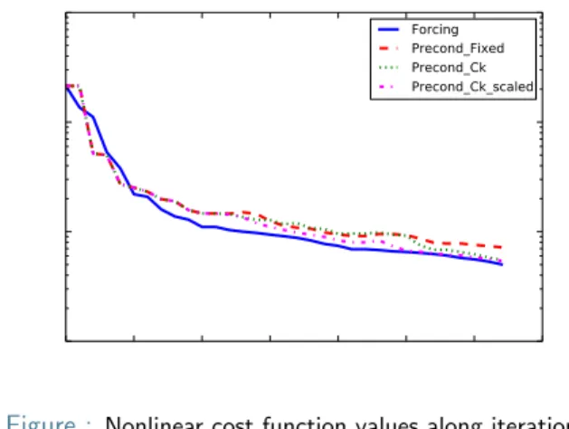
Numerical Results with OOPS qg-model

Figure : Nonlinear cost function values along iterations

!Last 8 pairs were used to construct the preconditioner ! B=↵vwT_(where _v₌_r

(69)

Weak contraints

Conclusion

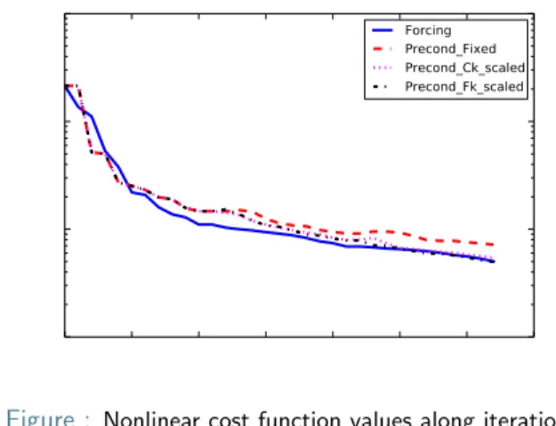
Numerical Results with OOPS qg-model

Figure : Nonlinear cost function values along iterations

!Last 8 pairs were used to construct the preconditioner Serge G. Large-scale inverse problems

(70)

Weak contraints

Conclusion

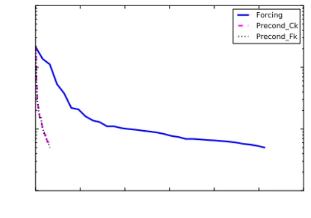
Numerical Results with OOPS qg-model

Figure : Nonlinear cost function values along sequential subwindow integrations

!At each iteration theforcing formulationrequires one application ofL 1_, followed by one application ofL T₍_{16 sequential subwindow integrations}₎

!At each iteration ofsaddle point formulationrequireone subwindow integration (provided thatL 1_and_L T _{are applied simultaneously)}

(71)

Weak contraints

Conclusion

Ensemble methods with a stochastic dynamical system Variational methods with a stochastic dynamical system

Summary, caveat and ongoing related work

(72)

Notations and toy example Subspace and model reduction Weak contraints

Conclusion

Conclusions

Very large scale higly-nonlinear forecasting problems can be solved

using dual methods, projection methods, satistical sampling,adapted

to nonlinearity

In some severe cases, having ”more” than a local minimum might be

needed. Model reductionand exploration techniques are useful

Most systems are a priori designed for solving the prediction problem. Using DA techniques to other settings not necessarily successful.

Further work. Errors between time-steps correlated. Having a parallel

codeis a challenge. Use nonlinear multigrid, domain decomposition

ideas forscalability.