PROJECT
NEREUS
Development of benchmarking
models for distribution system
operators in Belgium
FINAL REPORT
Disclaimer
This is an open report on the development of efficiency benchmarking models for electricity and gas distribution system operations in Belgium commissioned by la Commission de Régulation de l’Electricité et du Gaz (CREG), under the supervision of professors Per AGRELL and Peter BOGETOFT for SUM I C SI D A B.
The modeling and calculations in the report are based on confidential data material submitted to and obtained by the Commission de Régulation de l’Electricité et du Gaz (CREG). The calculations and estimates concerning other operators in this report do not constitute any statement of SUM I C SI D nor CREG concerning their absolute or relative performance. No numeric estimates of efficiency, costs or revenues in this report constitute regulatory rulings or the official viewpoint of the Commission de Régulation de l’Electricité et du Gaz (CREG).
Executive Summary
This report contains a methodological framework describing an economically sound
process for model specification and choice of econometric models for static and dynamic
efficiency for distribution system operators (DSO) in Belgium.
Principally, the objectives for this report are twofold.
First, it describes and motivates a systematic model specification process for the
identification, analysis and verification of a scientifically valid and economically sound
cost functions for the Belgian distribution of electricity and gas, respectively. This
process is guided by an overall system view to provide an output-oriented model that is
not only robust against multi-collinearity to improve precision, but also sufficiently
powerful as to provide unbiased estimates already as an average cost function. The
phase validates the obtained results using state-of-the-art statistical techniques for
regression robustness and the shape of the cost function. The resulting model is
validated against criteria for model development of regulatory efficiency models, leading
to extensions of scope for the chosen parameters. This phase is implemented on a panel
of Belgian DSO data and the resulting models are econometrically strong with a minimal
number of parameters and maximum explanatory power.
Electricity model
Gas model
Input:
Total expenditure (Totex) Total expenditure (Totex)Outputs:
Total number ofconnections (EAN) Total number of connections (EAN) Total circuit length of lines
(km) Total weighted length of pipelines (km) Total number of
transformers (#) Total number of pressure stations (#)
The fact that the models are symmetric is not imposed in the modeling, but a
consequence of two endogenous model specification processes.
The input in the cost function is total controllable expenditure (totex), including both
controllable operating expenditure and capital costs for depreciation and financial
charges. Costs related to charges for transmission services, transfers from previous
years, public service obligations and taxes are considered non-controllable and
deducted from the total expenditure. The input measure corresponds to regulatory
best-practice as it aligns to total operating cost independently of specific organizational
structures (such as the bias for asset ownership) and financial structure (such as the
bias for external financing). Totex is a sound long-term measure of the resources
mobilized for the provision of network services, granting the operators the right to
decide upon the optimal combination of asset ownership, financing and staff intensity as
to accomplish their tasks.
The inputs correspond to output dimensions that are true cost-drivers of total
expenditure, related to capacity provision and customer service.
The second objective is to review and suggest a methodology for regulatory efficiency
benchmarking for the CREG. Regulatory benchmarking is subject to strict criteria
concerning the methodological rigor, procedural equity and respect of the legal
framework for its implementation. Hence, a regulatory benchmarking model is one that
delivers estimates of the cost for “an efficient and structurally comparable network
operator” as a relevant long-term basis for tariff regulation. In particular, the national
regulator should ensure that the methodologies for tariff approvals provide the
distribution operators with appropriate incentives for short- and long-term efficiency in
network services, “it fosters market integration and security of supply and supports
related research activities”.
Consequently, we have to respect two perspectives on the design of a regulatory
benchmarking model. On the one hand the procedural requirements, fundamental to any
public regulation are: to proceed with conservative assumptions on technological and
cost structures, to base the rulings on revealed evidence rather then projections and to
implement models which are complete, verifiable and monotonous in the given task
description. On the other hand the socio-economic objectives stipulate that the model
should incite efficient operations and be compatible with a sound structural
development for the entire sector.
The recommended benchmarking methodology in this report is a set of non-parametric
Data Envelopment Analysis (DEA) models to be implemented using non-decreasing
returns to scale assumption and subject to three pre-determined filters for frontier
outlier detection. The two perspectives naturally support this conclusion in various
dimensions. First, DEA is based on classical production theory and is fundamentally an
inner cautious approximation of the production space, based on real observations with
an absolute minimum of assumptions. The approach is specifically suited to regulatory
applications in that it allows for an endogenous determination of the local substitution
(relative costs) for each operator in a sense that puts it in the best possible light. As
opposed to parametric models (e.g. SFA) where a certain number of assumptions need
to be ascertained and the numerical convergence is not guaranteed for all instances, DEA
constitutes a stable procedural tool to inform regulatory rulings under all circumstances.
Second, the DEA is founded on best-practice regulation, identifying and gauging the best
performers in a sector, rather than average-practice regulation, which is influenced by
the performance of inefficient operators and the incentive provision of which is at best
ambiguous if not perverse.
The DEA models, defined on the cost models specified in the first part of the projects, are
capable to inform regulatory rulings with two important elements for tariff reviews:
1.
Incumbent static inefficiency levels at a given reference year
The first information, the relative cost-efficiency in total expenditure, is vital to ensure
that tariffs reflect equal efforts in cost-reductions and do not constitute hidden transfers,
cross-subsidies or managerial slack. As for any regulated monopoly, the network
services should be performed using best-practice and the long-term costs should reflect
such practice, irrespective of which operator the captive client is assigned to.
The second information represents the fair sharing of the productivity gains in a sector
where certain exogenous price changes (inflation) are passed directly to the consumer.
However, rather than measuring and imposing the average productivity growth on all
firms, which would unfairly sum both the improvement of inefficient units (catch-up)
and the relatively more expensive and risky technological innovation by frontier firms
(technological change or frontier shift). Thus, to be consistent with the first objective
(procedural equity and diligence) the same methodology should be used on real data
from comparable firms to measure both static and dynamic efficiency. Moreover, to be
consistent with the second objective (long-term efficiency incentive provision), the
dynamic model must be capable to decompose observed productivity growth into the
components related to common frontier shift and the efficiency changes by individual
firms. Again, DEA is the most suitable integrated methodology to perform these two
objectives.
This project is intended as a white paper or a methodological roadmap for the
implementation of regulatory benchmarking to support the tariff methodology of the
CREG, also in the long run. The derived models are econometrically sound and exhibit
high model fit, the choice of benchmarking methodology is consistent, relevant and
effective with respect to the task, legislation and data. We note also that the overall
regulatory approach along these lines is consistent with international regulatory good
practice, further supporting the argument of its longevity.
While the reader might be curious to find final results for the derived models, for the
sector or their operator, the data material is not yet released for such analysis. However,
we remain certain that the results of the application of the methodology in this report
will be convincing, useful and informative for multiple uses.
Table of Contents
Disclaimer ... 2
1.
Organization ... 8
2.
DSO Regulation framework ... 10
2.1
Outline ... 10
2.2
Belgian Legislative Framework ... 10
3.
Benchmarking methods ... 14
3.1
Effectiveness, efficiency and productivity measures ... 14
3.2
Technology and cost estimation ... 19
3.3
Non-parametric models (DEA) ... 21
3.4
Parametric approaches ... 23
3.5
Engineering and accounting information ... 26
3.6
Data cleaning, structural corrections and sensitivity analyses ... 27
3.7
Analysis and conclusion... 30
4.
Criteria for model structure ... 31
4.1
Definitions ... 31
4.2
Output orientation ... 32
4.3
Structural correction... 33
4.4
The input measure ... 33
4.5
Economies of scope ... 34
4.6
Summary ... 35
5.
Methodology for model specification ... 36
5.1
Background ... 36
5.2
Variable selection criteria for regulatory use ... 36
5.3
Variable classification ... 37
5.4
Estimation procedure ... 37
5.5
Model specification procedure... 38
5.6
Banker test of model specification ... 39
5.7
Robustness ... 39
5.8
Age effect test ... 40
5.10
Economies of scale ... 41
6.
Model specification: electricity ... 44
6.1
Overview ... 44
6.2
Data ... 44
6.3
Variables ... 48
6.4
OLS stage – model size ... 49
6.5
Recursive regression – optimal model ... 50
6.6
Outlier analysis ... 53
6.7
Validation of Z-variables ... 55
6.8
Model specification results ... 57
7.
Model specification: gas ... 58
7.1
Overview ... 58
7.2
Data ... 58
7.3
Variables ... 59
7.4
OLS stage – model size ... 59
7.5
Recursive regression – optimal model ... 61
7.6
Outlier analysis ... 64
7.7
Validation of Z-variables ... 65
7.8
Model specification results ... 67
1.
Organization
1.01 This is a final report on the model development of benchmarking models for the economic regulation of energy distribution system operations in Belgium. The report is commissioned by the Commission de Regulation de l’Electricité et du Gaz (CREG), the federal energy regulatory authority in Belgium.
Project team
1.02 Project leader from SUM I C S I D is Senior Associate Prof. Dr. Per J. Agrell. The project team consisted also of senior associate Prof. Dr. Peter Bogetoft and associate Dr. Misja Mikkers,. 1.03 The Federal Regulator CREG through its Director for tariffs and accounts Guido CAMPS
appointed senior advisor Natalie CORNELIS and advisors Christine COBUT, An PIECK as the project team for NEREUS.
Background
1.04 The CREG together with Frontier Economics started in 2003 with developing a benchmarking tool specifically for the regulation of electricity utilities in Belgium. Based on the model developed in 2003 and part of 2004, the CREG proceeded in applying this same model for the gas utilities.
1.05 The first real application of the benchmarking model (based on DEA) was done on the 2005 tariff controls. Since then (2007), because of different problems with legislation and court cases the application of the benchmarking model was stopped.
1.06 With the introduction of the Third IEM Directive and the elaboration of powers for the National Regulatory Authority (NRA) the CREG has recently started public consultations on her proposals for tariff methods. These proposals contain the reintroduction of a benchmarking tool/model (based on DEA) in the tariff control.
1.07 Based on the 2005-2007 experiences, CREG is committed to continue with model-based regulation, where non-parametric efficiency estimates play a pivotal role. This project is a reactivation of the core model in the regulatory regime, involving both model specification, external and internal communication of its properties and software provision.
Objectives
1.08 This report on the NEREUS (Network Efficiency Regulation models for EUropean Systems) project aims at documenting
1) The development of theoretically and economically sound efficiency assessment models for electricity and gas distributors in Belgium
2) The analysis and choice of an efficiency assessment methodology for this application, capable of both static and dynamic analyses in line with the tariff methodology of CREG.
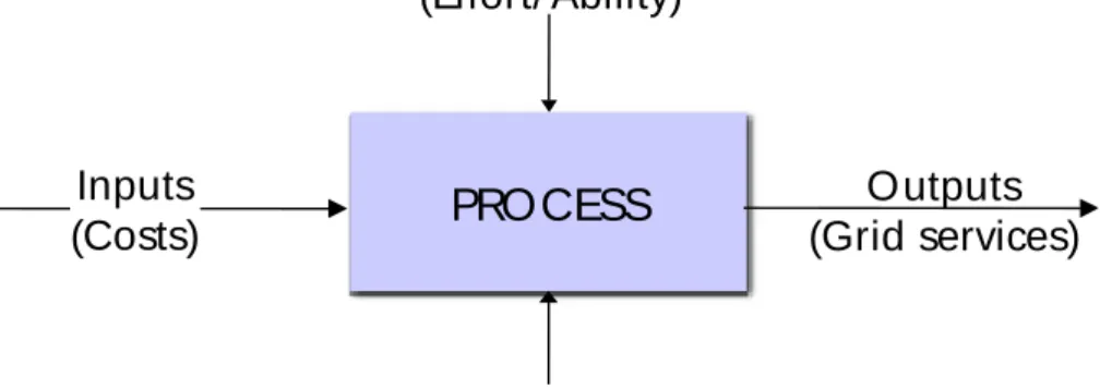
Process
1.09 The data collection in this project followed a formal procedure whereby data calls were issued to the DSO through CREG and data were delivered directly to CREG.
1.10 The confidentiality of the obtained information is recognized by the project team through the use of specific confidentiality clauses with all subcontracted staff, centralized storage of confidential information and separation and traceability of access to such information.
2.
DSO Regulation framework
2.1
Outline
2.01 The economic regulation of energy distribution is primarily determined by the following European directives:
DIRECTIVE 2009/72/EC OF THE EUROPEAN PARLIAMENT AND OF THE COUNCIL of 13 July 2009 concerning common rules for the internal market in electricity and repealing Directive 2003/54/EC (for electricity)
DIRECTIVE 2009/73/EC OF THE EUROPEAN PARLIAMENT AND OF THE COUNCIL of 13 July 2009 concerning common rules for the internal market in natural gas and repealing Directive 2003/55/EC; (for gas)
2.02 This regulation was created in the objective to realize a competitive electricity and gas market, to organize access to the networks and to install a regulating authority.
2.2
Belgian Legislative Framework
2.03 The federal government is responsible for "matters which, on account of their technical and economic indivisibility, must be dealt with on an equal basis at national level". This applies inter alia to energy transmission and particularly to the 150 to 380 kV transmission grid operated by Elia.
2.04 Regions are responsible for distribution and local transmission of electricity via networks with a nominal voltage of 70 kV or less. They are also responsible for renewable energy (except for offshore wind farms) and the rational use of energy (RUE).
2.05 The federal government is responsible for tariff policy for both transmission and distribution system operators.
2.06 The CREG as federal regulator has defined its methods1 for the calculation and determination
of tariff conditions relating to the connection and access to the electricity and gas distribution networks referred to in Article 37, Paragraph 6, a), of the European Parliament and Council Directive 2009/72/EC of 13 July 2009 concerning Community rules for the internal electricity market and the repeal of Directive 2003/54/EC (hereafter: Directive 2009/72/EC) and article 41, Paragraph 6, a), of the European Parliament and Council
1 Projet d’arrêté (Z)110908-CDC-1106 fixant les méthodes de calcul et établissant les conditions tarifaires
de raccordement et d’accès aux réseaux de distribution d’électricité visées à l’article 37, alinéa 6, a), joint à l’article 37, alinéa 1er, a), joint à article 37, alinéa 10 de la directive 2009/72/CE du Parlement européen et
du conseil du 13 juillet 2009 concernant des règles communes pour le marché intérieur de l’électricité et abrogeant la directive 2003/54/CE.
Projet d’arrêté (Z)110908-CDC-1107 fixant les méthodes de calcul et établissant les conditions tarifaires de raccordement et d’accès aux réseaux de distribution de gaz naturel visées à l’article 41, alinéa 6, a), joint à l’article 41, alinéa 1er, a), joint à article 41, alinéa 10 de la directive 2009/73/CE du Parlement
européen et du conseil du 13 juillet 2009 concernant des règles communes pour le marché intérieur du gaz naturel et abrogeant la directive 2003/55/CE.
Directive 2009/73/EC of 13 July 2009 concerning Community rules for the internal market in natural gas and the repeal of Directive 2003/55/EC (hereafter: Directive 2009/73/EC). 2.07 The implementation deadline for Directives 2009/72/EC and 2009/73/EC expired on 3
March 20112. The Belgian Government has not to date implemented these Directives. This
does however not imply that provisions of the existing regulatory framework which do not comply with these Directives can automatically continue to be applied.
2.08 In accordance with Article 35, Paragraph 1, of Directive 2009/72/EC and Article 39, Paragraph 1, of Directive 2009/73/EC, each Member State must appoint a single national regulatory body at national level. In Belgium, the CREG is the national regulatory body based on the Laws of 29 April 1999.
2.09 Article 37, Paragraph 1, of Directive 2009/72/EC and Article 41, Paragraph 1, of Directive 2009/73/EC define the primary task of the regulatory body as follows: “Determination or approval, according to transparent criteria, of transmission or distribution tariffs or of the calculation methods therefor”.
2.10 In accordance with Article 37, Paragraph 6, of Directive 2009/72/EC and Article 41, Paragraph 6, of Directive 2009/73/EC, the determination of the tariff setting method is an essential and exclusive attribution of the regulator. The option that existed under the second Directive for a tariff setting method to be submitted by the regulator to another body of the Member State in order to have it included in a formal decision is no longer available under the third Directives3. It is therefore no longer possible in Belgium to request the CREG to
submit a tariff setting method to the King in order to have it formalised by means of a Royal Decree.
2.11 The tariff conditions in effect (in particular Article 12octies of the Electricity Act4 and Article
15/5decies of the Gas Act5, as well as the Tariff Decrees of 2 September 20086) have
therefore also – and certainly since the expiry of the implementation deadline on 3 March
2 Article 49 of Directive 2009/72/EC and Article 54 of Directive 2009/73/EC.
3 See absence of equivalent, pursuant to Art. 37 & 41, Para. 6, of Directive 2009/72&73/EC, of a provision such as Art. 23 & 25, Para. 3, of Directive 2003/54&55/EC, as well as (a contrario) Art. 37 & 41, Para. 2, of Directive 2009/72&73/EC. See also the interpretive note of the European Commission dd. 22 January 2010: “The regulatory authorities”, pages 12-14 “Articles 37 of the Electricity Directive and 41 of the Gas Directive are the key Articles that provide for the duties of the NRA. [...] Some of the duties are to be fulfilled solely by the NRA (core duty); other duties can be carried out by other authorities [...] These core duties include: duties in relation to tariffs for access to transmission and distribution networks [...] Under Article 37(6)-(7) of the Electricity Directive and Article 41(6)-(7) of the Gas Directive, the NRA must be responsible for fixing or approving sufficiently in advance of their entry into force at least the
methodologies used to calculate or establish the terms and conditions for connection and access to national networks, provision of balancing services and access to cross-border infrastructures. [...] Under the second Electricity and Gas Directives, it was possible for the NRA to submit the tariff or the
methodology for formal approval to the relevant body of the Member State and for the relevant body to approve or reject the draft NRA decision. This is contrary to the provisions of the new Electricity and Gas Directives, which unequivocally establish that the NRA must be able to take decisions autonomously and that its decisions are directly binding”.
4 Law of 29 April 1999 concerning the organisation of the electricity market.
5 Law of 12 April 1965 concerning the transport of gaseous products and others by means of pipelines. 6 Royal Decrees of 2 September 2008 concerning the rules relating to the determination of and control of
2011 – come into conflict with Directives 2009/72/EC and 2009/73/EC to the extent that they determine the tariff setting method.
As a consequence of the principle of the priority of EU law, every governmental body is under the obligation not to apply national provisions that are in conflict therewith7.
2.12 The non-applicability of a national provision does not only exist if the provision is incompatible with a rule of EU law, but can also follow from the fact that the provision has come into being in conflict with a procedure dictated by EU law8. The conflict with a
Directive can obligate a government body not to apply national process or jurisdiction rules (that are prejudicial to the protection of the rights referred to in the Directive)9.
2.13 Based on the above, the CREG can, since 3 March 2011, no longer apply the tariff setting method as defined in Article 12octies of the Electricity Act6, Article 15/5decies of the Gas Act
and in the Tariff Decrees of 2 September 2008.
2.14 The Constitutional Court has also ruled that the law which confirmed the Tariff Decree of 2 September 2008 is in conflict with Article 37, Paragraph 6, a), of Directive 2009/72/EC, and that as a result of this provision it is no longer possible for the King to set the distribution tariffs upon proposal from the CREG, in view of the fact that the competence to do so has from then onwards exclusively been reserved to the CREG10. Because of the similarity
between the Tariff Decree on electricity and gas, these remarks also seem to apply to the Tariff Decree on gas.
2.15 The Council of State, Legislative Division, has, incidentally, and as concerns a preliminary bill “for the amendment of the Act of 29 April 1999 concerning the organisation of the electricity market and the Act of 12 April 1965 concerning the transport of gaseous products and others by means of pipelines”, issued the following opinion11:
“In any event, Article 37, Paragraph 10, of Directive 2009/72/EC offers the regulatory body the option to determine or approve the transmission and distribution tariffs as well as their calculation methods on a temporary basis and to issue a decision concerning appropriate compensation measures if the definitive transmission and distribution tariffs or calculation methods were to differ from such interim tariffs or calculation methods. The authors of the bill can, in accordance with this provision, provide for an option for the CREG to continue to apply the provisions of the two Royal Decrees to be repealed while waiting for a new regulation to be defined by the CREG. The fact that the repeal of the two abovementioned Royal Decrees results in a legislative vacuum does not however detract from the fact that since the expiry of the deadline for implementation of Directive 2009/72/EC it has become the role of the CREG to fill that vacuum and to determine by itself the necessary interim measures if the determination of the tariffs is delayed, either by deciding to use (specific aspects of) the old tariff setting methodology, or else by immediately providing for a temporary or a transitional regulation while waiting for a final regulation defined by it.”
7 [European] Court of Justice, 103/88 of 22 June 1989, Fratelli Costanzo, No. 33.
8 K. LENAERTS and P. VAN NUFFEL, European Law, Antwerp, Intersentia, 2011, page 520; [European]
Court of Justice, C-194/94 of 30 April 1996, C.I.A.
9 See e.g. [European] Court of Justice, C-118/00 of 28 June 2001, Larsy, No. 50-53. 10 Cf. Constitutional Court, decision No. 97/2011 of 31 May 2011, text item. B. 9. 5. 11 Opinion 49.570/3 of 31 May 2011, text item 38.1.
2.16 In addition, the Brussels Court of Appeal has also repeatedly ruled that EU law is against the regulatory body being held to comply with the standards and decisions of other governmental authorities in the exercise of its competences12.
2.17 Based on the absence of a timely and Directives compliant implementation in Belgium, the CREG aims to implement the task entrusted to it under European law by means of determining the methods for the calculation and determination of tariff conditions relating to the connection and access to the electricity and gas distribution networks.
2.18 Finally, the tariff methods also implement the Recommendation of the European Commission of 7 June 2011, ratified by the European Council on 24 June 2011, that Belgium should, in the period 2011-2012 take action in order to: “undertake measures to promote competition on the electricity and gas markets by further increasing the effectiveness of the industry regulatory and competition authorities.13”
2.19 The tariff methods are currently subject to public consultation and include both principles on the assessment of reasonableness of costs as well as an assessment model for cost control measures.
2.20 Directive 2009/72/EC (Article 37.8) and Directive 2009/73/EC (Article 41.8) state that, in fixing or approving the tariffs or methodologies, the regulatory authorities shall ensure that distribution system operators are granted appropriate incentive, over both the short and long term, to increase efficiencies. This precludes any automatic, integral approach to cost recovery. Rather, it requires a cost orientation, or “cost reflectivity.” Indeed, network operators must be required to achieve efficiency improvements on the basis of total cost control.
12 Cf. Brussels Court of Appeal, Ville de Wavre decision, of 15 June 2011, 2008/AR/1033, 2008/AR/1936,
2008/AR/2649, § 35 at the end, and the Tecteo decision of 29 June 2011, 2008/AR/147, 2008/AR/935, § 40 at the end: “the Community Law stipulations concerning the determination of the methods for the calculation of tariffs for the distribution of electricity and gas or of the tariffs for the said services are opposed to the principle that the regulator be forced, in the exercise of its functions, to follow the
3.
Benchmarking methods
3.01 In this chapter, we provide an introduction to start-of-the art benchmarking methods. Since there are by now many text-books covering the different types of benchmarking models and since many of these techniques are now used in regulation internationally at a routine basis, we do not seek to cover all possibly relevant methods in details.
3.02 Our aim is to give a basic vocabulary and idea about the approaches for readers without much previous exposure to this literature. Hence, we focus on the methods used in this report. Also, our aim is to point to some of the difficulties of these methods and the pre-and post analyses, e.g. initial data cleaning and post analyses sensitivity analyses, that are needed not the least in regulatory applications.
3.1
Effectiveness, efficiency and productivity measures
3.03 Ideally, a performance evaluation should measure effectiveness i.e. the extent to which it is possible to improve the overall goal we give to the evaluated. In reality, this is complicated since must organization pursues multiple goal that are not easily aggregated. Moreover, we generally lack the information about the possible transformation of resources to services of real organizations.
3.04 In real evaluations or benchmarking exercises, we therefore go from measuring effectiveness to efficiency, e.g. the ability to provide the same or more services with the same or less resources. Also, we go from absolute efficiency by measuring against an empirical norm as established by comparison with other units or by including information derived from actual practices. The latter corresponds to the establishment of an empirical model, and the former to the measurement of efficiency relative to the estimated model.
3.05 To be slightly more formal, assume that an organization, for now a DSO, has delivered a vector of outputs (services) yi using a vector of of inputs xi. Also, let the goal of the
organization be to maximize U(xi,yi) and the feasible combinations of (xi,yi) is the set T. Also,
let T* be an empirical approximation of T.
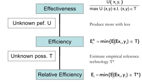
3.06 The logical moves from effectiveness to efficiency to relative efficiency can now be illustrated as in Figure 3-1 below
Figure 3-1 From effectiveness to relative efficiency
3.07 In this chapter we shall describe different ways in which we can establish the empirical model, or the estimated technology, T* above using statistical, programming, engineering and accounting methods. Before turning to these more specific details, however, it is useful to discuss the problem of measuring efficiency relative to a given technology.
Technical efficiency, cost efficiency and sub-vector efficiency
3.08 The literature suggest many possible productivity measures but for the purpose of this study, it suffices to define three concepts.
3.09 Technical efficiency is a question of the possibility to expand some or all outputs or reduce some or all inputs. The typical Farrell measure is the one indicated in Figure 3-1, namely
= minimal common fraction of all inputs that suffices to produce the
given output.
3.10 When there is only one input, namely costs ci,, Ei becomes the fraction of costs that is needed
to produce the given output yi in the given technology. We call this the cost efficiency, CE
= Minimal costs / Actual costs
3.11 The relationship between costs and inputs are given by ci = wxi, where w is a vector of factor
prices. We see therefore that cost efficiency not only evaluates whether given factors are used in the most efficient way, technical efficiency, but also to what extent the factor mix is optimal given the relative prices and the technological possibilities to substitute between them, so-called allocative efficiency. For example, CEi =0.9 means that it is possible to save
10% of the actual costs.
3.12 A third efficiency concept of direct relevance to the present task is that of sub-vector efficiency. The idea is that some inputs factors may be controllable but others not (in the
(non-controllable) assets are of good quality, for example, this may lead to lower operating costs. To cope with such interdependencies without presuming that everything can be changes, one can use the sub-vector efficiency. Letting be the controllable (discretionary) inputs and the the non-controllable (fixed) inputs, sub-vector efficiency becomes
= minimal common fraction of all controllable inputs that together with
the non-controllable inputs suffices to produce the given outputs
3.13 The interaction between controllable and non-controllable inputs (or costs) has implicationsfor regulation. It means for example that a revenue cap ideally should be fixed in view of the capital costs allowed
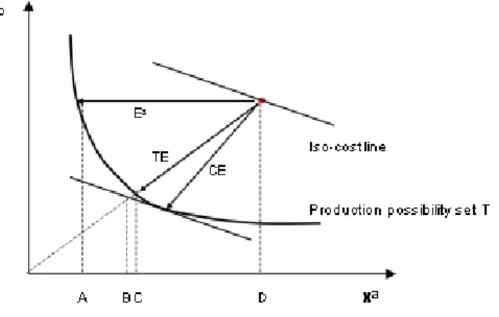
3.14 The three efficiency concepts are illustrated in Figure 3-2Fout! Verwijzingsbron niet gevonden.. TE corresponds to C/D, CE corresponds to B/D and if xa is assumed to be
non-discretionary, the sub-vector efficiency ES is A/D.
Figure 3-2 Efficiency concepts
Malmquist dynamic productivity analysis
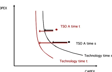
3.15 Over time, both the behavior of an individual DSO and the nature of the technology changes. This is illustrated in Figure 3-3 below.
Figure 3-3 Dynamics of production frontiers at times s and t
3.16 In the scientific literature productivity refers to changes over time. If outputs change more than inputs, productivity improves. The standard approach to dynamic evaluations is to use so-called Malmquist indices. They measures the change from one period to the next by the geometric mean of the performance change relative to the past and present technology. 3.17 Specifically, let Ei(s,t) be a measure of the performance of DSOi in period s against the
technology in period t. Now, DSOi ‘s improvement from period s to period t can be evaluated
by the Malmquist index Mi(s,t) given by
3.18 The intuition of this index runs as follows. We seek to compare the performance in period s
to period t. The base technology can be either s or t technology, so we take geometric mean. Improvements make nominator larger than denominator. Hence, M > 1 corresponds to progress and for example M = 1.2 would suggest a 20% improvement from period s to t, i.e. a fall in the resource usage of 20%.
3.19 The change in performance captured by the Malmquist index may be due to two, possibly enforcing and possibly counteracting factors. One is the technical change, TC, that measures the shift in the production frontiers corresponding to a technological progress or regress. The other is the efficiency change EC which measures the catch-up relative to a fixed frontier. This decomposition is developed by a simple rewrite of the Malmquist formula above given by
3.20 Again the interpretation is that values of TC above 1 represent technological progress – more can be produces using less resources – while values of EC above 1 represents catching-up, i.e. less waste compared to the best practice of the year.
3.21 The Malmquist measure and its decomposition is useful to capture the dynamic developments from one period to the next. Over several periods, one should be careful in the interpretation. One cannot simply accumulate the changes since the index does not satisfy the so-called circular test, i.e. we may not have M(1,2) x M(2,3) = M(1,3) unless the technical change is so-called Hicks-neutral. This drawback is shared by may other indices and can be remedies by for example using a fixed base technology. This however, is beyond the scope of this report.
Incumbent inefficiency and frontier shift
3.22 The efficiency and productivity measures above allow us to measure both the incumbent inefficiency, i.e. the excess usage of resources in a given period, of a DSO and the technological progress (or regress) of the industry, i.e. a reasonable dynamic trajectory. This is illustrated in Figure 3-4 below.
Figure 3-4 Incumbent inefficiency and frontier shifts
3.23 So far, we have measured performance and progress presuming that the cost function or technology was given. What remains is to describe state of the art in cost function modeling.
TFP measures with given prices
3.24 We close this discussion of basic measures of efficiency and productivity with a brief introduction to the Total Factor Productivity (TFP) index that can be used to estimate productivity improvement rates for use in generalized X-factor determination, or to evaluate ex post productivity improvement in yardstick regimes. TFP is frequently used in incentive regulation in the US and in price-cap regulation in the Anglo-saxon tradition (e.g. New Zealand in Lawrence and Diewert, 2006).
3.25 Below a brief description is given of the approach. For an excellent introduction to TFP estimations in regulation, see Coelli, Estache, Perelman and Trujillo (2003), further examples of studies are presented in Coelli and Lawrence (2006).
3.26 Productivity is in general defined as the ratio of outputs to inputs. The Total Factor Productivity is an extension to the case of multiple inputs and outputs:
3.27 where Y is the proportional change in output quantity and X is the corresponding change in input quanta. The multiple dimensions are weighted according to some set of weights, the most popular being the Fisher ideal index (Diewert, 2004) that uses (exogenously given) prices. The total factor productivity growth from a base year 0 to a later year t is obtained as:
3.28 where is the price for output i in the base period 0, is the price of output i in period t
= 1,..,T, and are the output quantities of item i in periods 0 and t, respectively, and are the input prices for input i in periods 0 and t, respectively, and and are the quantities of input i in periods 0 and t, respectively. The summation indexes i and k are covering the same range of all inputs and outputs, respectively.
3.29 The square-root expression above can be avoided by using the logarithmic form of TFP; i.e.:
3.30 An obvious challenge with the TFP method is to obtain an a priori set of valid market prices for all outputs, i.e. prices that should reflect a profit maximizing behavior. In the case of infrastructure regulation, these prices are normally endogenous from the regulation, the objectives may be mixed or unclear and there are several other methodological problems with the exact interpretation of the input prices.
3.2
Technology and cost estimation
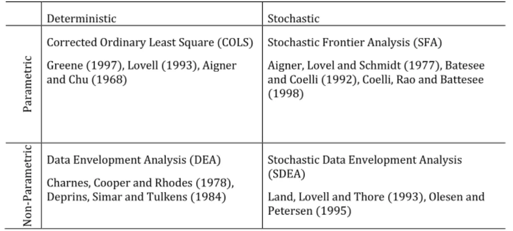
3.31 Econometrics has provided a portfolio of techniques to estimate the cost models for networks, illustrated in Table 3-1 below. Depending on the assumption regarding the data generating process we divide the techniques in deterministic and stochastic, and further depending on the functional form into parametric and non-parametric techniques.
Table 3-1 Model taxonomy Deterministic Stochastic Pa ra m et ri c
Corrected Ordinary Least Square (COLS) Greene (1997), Lovell (1993), Aigner and Chu (1968)
Stochastic Frontier Analysis (SFA) Aigner, Lovel and Schmidt (1977), Batesee and Coelli (1992), Coelli, Rao and Battesee (1998) Non -Pa ra m et ri c
Data Envelopment Analysis (DEA) Charnes, Cooper and Rhodes (1978), Deprins, Simar and Tulkens (1984)
Stochastic Data Envelopment Analysis (SDEA)
Land, Lovell and Thore (1993), Olesen and Petersen (1995)
3.32 Corrected ordinary least square (COLS) corresponds to estimating an ordinary regression model and then making a parallel shift to make all units be above the minimal cost line. Stochastic Frontier Analysis (SFA) on the other hand recognizes that some of the variation will be noise and only shift the line – in case of a linear mean structure – part of the way towards the COLS line. Data Envelopment Analysis (DEA) estimates the technology using the so-called minimal extrapolation principle. It finds the smallest production set (i.e. the set over the cost curve) containing data and satisfying a minimum of production economic regularities. Like COLS, it is located below all cost-output points, but the functional form is more flexible and the model therefore adapts closer to the data. Finally, Stochastic DEA (SDEA) combines the flexible structure with a realization, that some of the variations may be noisy and only requires most of the points to be enveloped.
3.33 A fundamental difference from a general methodological perspective and from regulatory viewpoint is the relative importance of flexibility in the mean structure vs. precision in the noise separation. This means that there are basically two risks for error that cannot be overcome simultaneously. These are 1) risk of specification error, and 2) risk of data error.
Specification error
3.34 The inability of the model to reflect and respect the real characteristics of the industry is related to the specification error. Avoiding the risk of specification error requires a flexible model in the wide sense. This means that the shape of the model (or its mean structure to use statistical terms) is able to adapt to data instead of relying excessively on arbitrary assumptions. The non-parametric models are by nature superior in terms of flexibility.
Data error
3.35 The inability to cope with noisy data is called data error. A robust estimation method gives results that are not too sensitive to random variations in data. This is particularly important in yardstick regulation with individual targets – and less important in industry wide motivation and coordination studies. The stochastic models are particularly useful in this respect.
3.36 It is worthwhile to observe that the two properties may to some extent substitute each other. That is, the flexible structure allowed by non-parametric deterministic approaches like DEA may compensate for the fact that DEA does not allow for noise and therefore assigns any deviation from the estimated functional relationship to the inefficiency terms. Likewise, the
explicit inclusion of noise or unexplained variation in the data in SFA may to some extent compensate for the fact that the structural relationships are fixed a priori, i.e. the noise terms may not only be interpreted as a data problem but also as a problem in picking the right structural relationship. As an illustration of this it has been found that the SFA efficiencies are often larger than the DEA efficiencies as long as the model is somewhat ill-specified., i.e. the inputs and outputs are badly chosen. The reason is that SFA in this case assigns the variations to the noise term while DEA assigns everything to the efficiency term. As the model is extended to include more relevant inputs and outputs, the two methods have been found to produce quite comparable results.
3.3
Non-parametric models (DEA)
3.37 The basic DEA (Data Envelopment Analysis) formulation for a unit 0 in a set of p
comparators using a process model with m inputs and n outputs would be
where denotes the reference set of comparators (i.e. all units but 0 if super-efficiency, otherwise all units), r is the assumption regarding returns-to-scale (crs, vrs, nirs, etc), 0 is the unit under study, is the radial efficiency score and X and Y are (m x p) and (n x p) matrices for the input and outputs, respectively.
Reference set
3.38 The reference set may include all p observations to determine a frontier that includes the unit under evaluation (0). An additional possibility to extend the reference set with constructed observations from e.g. engineering norm models, ’ = . In this manner, an otherwise sparse dataset can still be used for non-parametric incentive provision. In the case reference set includes time series data, care should be taken to correct the economic measures for price changes during the period.
Returns to scale
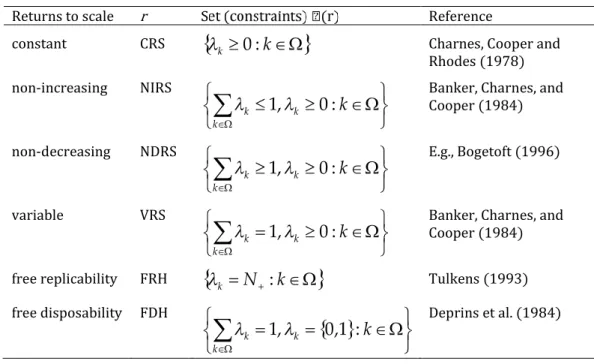
3.39 One of the few a priori assumptions of the non-parametric models includes the returns to scale for the technology. The literature lists the specifications constant returns to scale (crs), non-increasing returns to scale (nirs), non-decreasing returns to scale (ndrs), variable returns to scale (vrs), free replicability hull (frh) and free disposability hull (fdh). Table 3-2 presents a list of the most used assumptions along with their technical inclusion as one or two constraints in the DEA problem above.
Table 3-2 Returns-to-scale assumptions in DEA-models with some references.
Returns to scale r Reference
constant CRS Charnes, Cooper and
Rhodes (1978)
non-increasing NIRS Banker, Charnes, and
Cooper (1984)
non-decreasing NDRS E.g., Bogetoft (1996)
variable VRS Banker, Charnes, and
Cooper (1984)
free replicability FRH Tulkens (1993)
free disposability FDH Deprins et al. (1984)
Orientation
3.40 Most applications in incentive regulation concern input-oriented models with an underlying assumption of cost-minimization over a set of endogenous (controllable) inputs. However, the non-parametric model can be adapted to the setting of output maximization (e.g. maximum utilization of a costly infrastructure with sunk capital, such as a district heating networks). The corresponding formulation is is
3.41 where denotes the reference set of comparators (i.e. all units but 0 if superefficiency, otherwise all units), r is the assumption regarding returns-to-scale (crs, vrs, nirs, etc), 0 is the unit under study, is the radial efficiency score and X and Y are (m x p) and (n x p) matrices for the input and outputs, respectively.
3.42 The non-parametric frontiers such as DEA, mostly presented as input-oriented technical or cost-efficiency formulations with national reference sets are popular tools for the implementation of incentive regulation in networks. Among countries relying completely or partially on such tools in 2007 we find for electricity distribution Austria, Belgium, Finland, Germany, Iceland, Norway, Sweden, for gas distribution Germany and Belgium.
3.4
Parametric approaches
3.43 In the parametric SFA approach, the separation of noise and inefficiency is technically done by assuming that the noise is two sided and inefficiency is one sided. Inefficiency makes costs increase and makes production fall short of the best possible, while noise may also lower the observed costs or increase the observed output. In addition to having one- and two sided deviations, the separation of noise and inefficiency is accomplished by making specific assumptions about the nature of the distributions, e.g. normal and half normal.
3.44 In the parametric approach, one also makes specific assumptions about the type of relationship between the inputs and outputs. The so-called functional form may for example be linear, log-linear or translog. We shall return to these assumptions below.
3.45 To be more specific, we may distinguish between three combinations of noise and inefficiency. Namely pure noise models, pure efficiency models and combined models. In a cost setting, we may assume that costs, x, depend on a series of output driver, y, as well as on a combination of the inefficiency term u ≥ 0 and the noise term v for each of the operator i
3.46 Pure noise (Ordinary least squares (OLS), average cost function): xi = C(yi) + vi
3.47 Pure inefficiency (Deterministic frontier):
xi = C(yi) + ui
3.48 Combined (Stochastic frontiers):
xi= C(yi) + ui + vi
3.49 In the specifications above, C(y) is the minimal cost function. It defines the least expensive way to provide the outputs y. The functional form of C(y) is given, except for some unknown parameter values , i.e. one uses C(y, ). The statistical analysis seeks to estimate the functional relationship, i.e. , and to estimate the inefficiencies, i.e. ui.
OLS approaches
3.50 The first of these specifications (OLS) is the specification in classical statistics. It fits a function to the data in such a way that the positive and negative deviations are as small as possible. The standard measure of goodness-of-fit is the sum of squares of deviations, which is why this approach is often referred to simply as the OLS, ordinary least squares approach. Since the OLS approach does not work with the idea of individual inefficiencies, the usage of OLS in regulation is problematic. It can of course be used to identify likely cost drivers and to evaluate structural inefficiencies. Individual inefficiencies, however, are by assumption absent. OLS is normally used as a preparatory step to find cost drivers for variable selection.
Stochastic Frontier Analysis
3.51 The stochastic frontier approach was introduced independently by Aigner, Lovell and Smith (1977) and Meuser and Van den Broeck (1977). This section provides a short introduction to the basic characteristics of SFA. A comprehensive introduction to SFA can be found for example in Coelli et al. (1998).
3.52 The key feature of SFA is that it allows for both noise and inefficiency. In a cost function interpretation, it would specify the costs as
where the inefficiency ui is distributed as a half-normal N+(0, σu2) and the noise term vi is
assumed normally distributed N(0, σv2).
3.53 Conceptually, it is attractive to allow for the realistic existence of both noise and inefficiency. The drawback of the approach is on the other hand that we need a priori to justify 1) the distribution of the inefficiency terms and 2) the functional form of the frontier.
3.54 The SFA specification is also attractive by allowing the use of classical statistical approaches like maximum likelihood estimation, likelihood ratio testing etc. In a SFA approach, we use the data to come up with a best estimate of the underlying costs function C. Compared to DEA, we have less freedom in our choices since we have to decide already at the outset about a possible classes of such functions. Given a best estimate of the cost function C, we can determine the noise plus inefficiency by comparing the actual cost and the cost function value.
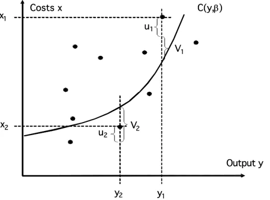
Figure 3-5 Stochastic frontier (both noise v and inefficiency u)
Inefficiency distribution
3.55 SFA requires some a priori assumption about the distribution of the inefficiency term in order to separate noise and uncertainty. It is hard to give strong arguments for a specific form like the half normal. It is therefore better to start with a more general and more flexible specification and to let the data reveal as closely as possible the correct distribution. We use the accepted general practice to assume that ui is truncated normal; N+(µ, u2), i.e. a normal
distribution centered around µ and next truncated to be above zero.
Functional forms of a cost function
3.56 The second fundamental problem in a parametric frontier approach is to select a functional form for the frontier. The selection of functional form is guided by intuition and data as well as theory. An experienced statistician is usually good at choosing functional forms with possibly data transformations and the sufficient degrees of freedom to provide a reasonable
DSO 1
goodness of fit of the data at hand. In addition, theory guides the selection by imposing reasonable properties on the estimated function, e.g. that costs function is homogenous in prices or that output sets are convex. A good general principle is to use the simplest possible representation with the sufficient flexibility to represent data. The simplest possible form is the linear one and a good starting point – and even a starting point used in the iterative procedures used to estimate more advanced forms – is therefore recommended to do a linear regression of cost on the different outputs.
3.57 A slightly more complicated specification is the log-linear one being linear in the log of the variables, corresponding to a multiplicative relationship in the original variables, well-known from Cobb-Douglas type functions.
3.58 Linear specifications correspond to first order approximations and the natural next step towards a workable form is to use quadratic approximations, possibly in the log of the variables.
3.59 A second order approximation using log variables gives the so-called translog form. In a cost function specification with n outputs and no prices, it pictures the relationship as
where Ci is the total cost of the i-th unit, yij is the j-th output quantity of the i-th unit, and the
b’s are unknown parameters to be estimated.
Summing up
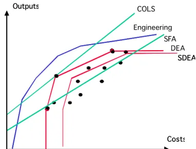
3.60 Figure 3-6 illustrates the approaches. Corrected ordinary least square (COLS) corresponds to estimating an ordinary regression model and then making a parallel shift to make all units be above the minimal cost line. Stochastic Frontier Analysis (SFA) on the other hand recognizes that some of the variation will be noise and only shift the line – in case of a linear mean structure – part of the way towards the COLS line. Data Envelopment Analysis (DEA) estimates the technology using the so-called minimal extrapolation principle. It finds the smallest production set (i.e. the set over the cost curve) containing data and satisfying a minimum of production economic regularities. Assuming free disposability and convexity, we get the DEA model illustrated in Figure 3-6. Like COLS, it is located below all cost-output points, but the functional form is more flexible and the model therefore adapts closer to the data. Finally, Stochastic DEA (SDEA) combines the flexible structure with a realization, that some of the variations may be noisy and only requires most of the points to be enveloped.
Figure 3-6 Benchmarking methods (example)
3.5
Engineering and accounting information
3.61 An obvious difficulty with the frontier approaches is that they require assessing a reasonable large number of comparators. In the case of a DSO, this may not be possible – at least not for all parts of its activities.
3.62 It is important to understand therefore, that the data used in the above models and in the programming methods in particular need not only be data from similar entities. Expert information and information derived partial models of different processes can also be included into the models. This can be done in both a primal and a dual way.
Inclusion of primal information
3.63 If engineers or accountants can construct production plans, i.e. input-output combinations, (xe,ye) that can be documented to be feasible even though they are never realized, they can
be included as any other realized production plan in the estimation process. This is particularly easy in the programming approach since such experimental entities simply enters as additional columns in the LP problem. In the statistical approaches, the consequences are more complicated since the data generation of the artificial units are obviously different from the actual observations making the final statistical inference problematic .
Inclusion in dual
3.64 The other approach is to use the accounting and engineering information about the relative importance or and costs of different outputs and production factors to create fewer aggregated outputs or inputs before the above programming and statistical approaches are used. Technically, this corresponds to using linear mappings of the inputs and outputs into vectors of smaller dimensions, , and and to build the programming and statistical models hereon.
3.65 This approach can be generalized to involve partial information about the relative importance of alternative cost drivers and the relative costs of alternative factors. In the
programming framework, this is implemented by using linear restrictions on the dual multipliers. In the statistical tradition, it is implemented in the Bayesian approach. Such generalizations are however beyond the scope of this report. Instead we shall look at a special case, namely the unit cost approach below.
More advanced models
3.66 The engineering approach can be extended into a full scale alternative to the empirical cost estimations using technical norm models like Model Networks or Reference Networks. 3.67 The idea of a Model Network Analysis (MNA) is to make a small planning model for a
theoretical case (e.g. mountainous transmission) and the to vary some variables (e.g. load, density) to document how it affects Capex and Opex. The approach has mainly been used in DSO contexts but can also be used in DSO settings. The outcome of such an exercise is to get estimates for complexity (e.g. assuming a base-case load; what is the factor for high load grid) and estimates for functional form, (e.g. what happens with CAPEX when the peak demand increase). It is normally used as environmental variables in benchmarking or yardstick models to reduce complexity. This approach has been used to generate exogenous variable in Austria (DEA) and to validate cost drivers in Germany (DEA/SFA) (Agrell and Bogetoft, 2007).
3.68 The aspiration of a Network Reference Model (NRM) is more ambitious since it works around the idea of creating full, more or less ideal grids. More specifically, departing from individual grid data (GIS) for each load point and task, such models find an estimate of the physical asset base (grid assets) needed to serve the exact area. It has been used for DSO regulation in Spain (BULNES/PECO, cf. Grifell-Tatje and Lovell, 2000) and Sweden (NPAM, cf. Larsson, 2003), cf. the case studies in Agrell and Bogetoft (2006a).
Unit cost approach
3.69 The idea of the unit cost approach is very simply. If we consider the set of assets A as the cost drivers, if we assume that the cost of operating one units of asset a is wa, and if we assume
that a DSO has an asset base given by the vector N, where Na is the number of assets a, then
the norm cost is simply assumed to be
3.70 The cost norm derived in this way is sometimes refereed to as the Net Volume or SizeOfGrid. Depending on the interpretation of the weights – e.g. if the are reflecting the total, the operating or the capital cost of one unit of the assets, this approach can be used to derive Totex, Opex and Capex efficiency measure, cf. Agrell and Bogetoft(2006b).
3.71 It is important to observe that this approach is based on implicit assumptions of constant return to scale, functional independence and constant marginal rate of substitution among the asset categories. The unit cost approach is used in e.g. assessment of transmission system operators, given the high asset specificity.
3.6
Data cleaning, structural corrections and sensitivity
analyses
3.72 The cleaning of data is a major effort in any regulatory application of the above methods. Likewise, the post analyses sensitivity analyses are important to correct for any reaming
briefly outline some of important data cleaning and sensitivity analyses techniques in this section.
Outlier analyses
3.73 Outlier analysis consists of screening extreme observations in the model against average performance. Depending on the approach chosen (OLS, DEA, SFA), outliers may have different impact. In DEA, particular emphasis is put on the quality of observations that define best practice. The outlier analysis in DEA can use statistical methods as well as the dual formulation, where marginal substitution ratios can reveal whether an observation is likely to contain errors. In SFA, outliers may distort the estimation of the curvature and increase the magnitude of the idiosyncratic error term, thus increasing average efficiency estimates in the sample. In particular, observations that have a disproportionate impact (influence or leverage) on the sign, size and significance of estimated coefficients are reviewed using a battery of methods that is described below.
3.74 In non-parametric methods, extreme observations are such that dominate a large part of the sample directly or through convex combinations. Usually, if erroneous, they are fairly few and may be detected using direct review of multiplier weights and peeling techniques. The outliers are then systematically reviewed in all input and output dimensions to verify whether the observations are attached with errors in data. The occurrence and impact of outliers in non-parametric settings in mitigated with the enlargement of the sample size. Thus, the number of validated units in the analysis for both electricity and gas has continuously been increased during the project. More on the actual implementation of these tests is found below.
3.75 In parametric methods, we are concerned with observations for which the x-value is extremely large, meaning that they have a potential leverage in influencing the shape and slope of the regression and that are off-center in the meaning that they actually exercise their leverage. In Agrell and Bogetoft(2007) we describe four diagnostic functions that can be used in automated outlier analysis in the regression phase, whereof Cook’s distance, is used in this project.
Outlier detection in DEA
3.76 The identification of DMU (Decision Making Unit) to check more carefully has used in particular four approaches.
3.77 One is to identify the number of times a DMU serves as a peer unit for other DMUs, peer counting. If a DMU is the peer for an extreme number of units, it is either a very efficient units – or there may be some mistakes in the reported numbers.
3.78 The other approach is to investigate the impact on average efficiency from unilateral elimination of the DMUs, efficiency ladders. If the elimination of one DMU leads to a significant increase in the efficiency of sufficiently number of units, there are again good reasons to check this unit more carefully.
3.79 Thirdly, we have done so-called shell analysis where the idea is to study the impact of groups of DMU, like the ones in the first shell, the second shell etc, cf also Agrell and Bogetoft(2002a). As the cost function is peeled this way, one shall check the shells with a significant impact on efficiency while there is less reason to continue the controls when the average efficiency is only improving slightly when a shell is eliminated.
3.80 Finally, we have used efficiency calculations to determine units with extreme super-efficiencies that are often associated with outliers, c.f. Banker and Chang(2005). Other
outlier detection methods designed with particular focus on frontier models have also been considered, for example Wilson(1993).
Bias correction
3.81 DEA models provide cautious estimates of the saving potentials and cost inefficiencies. This is one of the attractive features of DEA and is part of the theoretical foundation for the optimality of DEA based yardstick competition, cf. Bogetoft(1997,2000). If the model structure and the variables are chosen correctly, it means that no-one will be required to produce at costs that are below the truly minimal ones. In the terminology of incentive theory, the outcome is individually rational.
3.82 The back-side of the cautiousness is that the cost efficiency is biased upwards. On average, the units will look more efficient than they really are. This may be a problem in terms of the sharing of benefits between consumers and firms. It is however the price one must pay to avoid that an evaluated organization are faced with too hard terms.
3.83 Recent theoretical developments have taught us how to correct for this bias, namely via boot-strapping. In consequence, we can – following the literature initiated by Simar and Wilson(2000) - determine bias corrected efficiency scores, i.e. scores that are not biased. Moreover, using bootstrapping, we can determine confidence intervals around the bias corrected efficiencies.
Structural corrections
3.84 The relative performance evaluation of the DSO shall ideally be corrected for difference in the structural conditions. Thus, a DSO forced to live with the difficulties of special climate, topology, particularly dispersed costumers etc shall not be compared directly with DSO without these challenges. There are several ways to correct for such differences and to test their importance.
3.85 In a DEA framework, ordinal structural variables can be used to group the DSO and to only compare a DSO against DSOs working under less favorable conditions. If the structural variables are interval scaled, we can instead include them as pseudo non-controllable inputs or outputs.
3.86 Another and more common approach is to rely on second stage analyses. In a second stage analysis, the efficiency scores are regressed against the structural variable to determine the general impact of these. Next the efficiencies are corrected for the impact of these variables using the regression model. Often, an OLS estimation is used, but if one analyzes ordinary efficiencies as opposed to superefficiencies, one should ideally take into account the truncated nature of the dependent variable, the efficiency, i.e. one should use a truncated regression a la Simar and Wilson (2004) or a TOBIT regression following Tobin(1958). 3.87 In an SFA framework, the correction for structural variables can be handled as an integral
part of the maximum likelihood estimation by parameterizing the inefficiency distribution with such variables, cf. Batese and Coelli (1992). This approach seems to be superior to second-stage analyses, cf. Coelli and Perelman(1999).
3.88 In some case, we are not interested to correct the efficiency scores for the structural variables but we are interested to know if the model is biased against one type of DSO rather than another, e.g. bias in asset age due to nominal capital values. In such cases, one can – in addition to the second stage regressions – make non-parametric tests – like classical Mann-Witney and Kruskal and Wallis tests.
3.7
Analysis and conclusion
3.89 Given that the current mission concerns a national benchmarking and in view of the merits of the non-parametric approaches for regulatory applications, as discussed above, we recommend using DEA models to analyze the incumbent and dynamic efficiency for electricity and gas distribution operations in Belgium.
3.90 Following the theory of DEA, the number of cost drivers should not be greater than necessary to adequately reflect the heterogeneity in the production space. Also, in terms of returns to scale, conceptual reasoning and international experience would suggest using a non-decreasing returns to scale specification. The returns to scale assumption as well as alternative model specifications can however also be analyzed and tested using the Banker tests for model specification. We will do so, but we will also acknowledge that the asymptotic properties of these tests are only approximate when used on samples with a number of DSOs like in Belgium. The conceptual soundness of the specification and the results of the econometric average cost model specification shall therefore also be allowed an important role in the choice of model.
3.91 In terms of outlier identification and elimination, the sensitivity to outliers when frontier models are used suggest taking a cautious approach. Specifically, we suggest using three outlier detection and elimination criteria. First, we apply an econometric outlier detection criteria based on Cook’s distance, as done earlier in the model specification phase.
3.92 Secondly, a frontier based criteria based on the Banker super-efficiency tests. Specifically, we suggest using the relatively strict criteria that have also been used in the regulatory benchmarking of German electricity and gas DSOs. Let E(k,I) be the efficiency of k when all DSO are used to estimate the technology and let E(k;I\i) be the efficiency when DSO i does not enter the estimation. Now the super-efficiency elimination criteria remove DSO i from the reference set when
E(i;I\i) >q(0.75)+1.5*(q(0.75)-q(0.25))
where q(a) is the a fractile of the distribution of super-efficiencies, such that e.g. q(0.75) is the super-efficiency value that 75% has a value below.
1.01 Thirdly, we use the Banker F test approach like in the German regulatory implementation. The idea is to eliminate DSO i if it has an extreme impact on the efficiency of a large number of other DSO. This is implemented by considering the test indicator
3.93 Small values of this as evaluated in a F(n-1,n-1) distribution, c.f Banker(1996), will be an indication that i is an outlier.
Recommendation
3.94 For the dynamic analysis, we recommend using frontier shift based on DEA models to evaluate the general productivity development, i.e. the improvements realized and expected also of the frontier DSOs. Based on the same underlying model it provides a more consistent foundation for regulatory choices of incumbent and dynamic efficiencies, that they are.