Classification of incomplete patterns based on fusion of belief functions

Classification of incomplete patterns based on fusion of

belief functions

Zhun-Ga Liu, Quan Pan, Jean Dezert, Arnaud Martin, Gregoire Mercier

To cite this version:

Zhun-Ga Liu, Quan Pan, Jean Dezert, Arnaud Martin, Gregoire Mercier. Classification of

incomplete patterns based on fusion of belief functions. The 18th International Conference on

Information Fusion, Jul 2015, Washington, United States.

<

http://fusion2015.org/

>

.

<

hal-01270251

>

HAL Id: hal-01270251

https://hal.archives-ouvertes.fr/hal-01270251

Submitted on 6 Feb 2016

HAL

is a multi-disciplinary open access

archive for the deposit and dissemination of

sci-entific research documents, whether they are

pub-lished or not.

The documents may come from

teaching and research institutions in France or

abroad, or from public or private research centers.

L’archive ouverte pluridisciplinaire

HAL

, est

destin´

ee au d´

epˆ

ot et `

a la diffusion de documents

scientifiques de niveau recherche, publi´

es ou non,

´

emanant des ´

etablissements d’enseignement et de

recherche fran¸

cais ou ´

etrangers, des laboratoires

publics ou priv´

es.

Classification of incomplete patterns

based on fusion of belief functions

Zhun-ga Liu

, Quan Pan

, Jean Dezert

, Arnaud Martin

, Gregoire Mercier

1. School of Automation, Northwestern Polytechnical University, Xi’an, China. Email: [email protected] 2. ONERA - The French Aerospace Lab, F-91761 Palaiseau, France. Email: [email protected] 3.IRISA, University of Rennes 1, Rue E. Branly, 22300 Lannion, France. Email: [email protected] 4. Telecom Bretagne, CNRS UMR 6285 Lab-STICC/CID, Brest, France. Email: [email protected]

Abstract—The missing values in the incomplete pattern can either play a crucial role in the class determination, or have only little influence (or eventually none) on the classification results depending on the different cases. A fast classification method for incomplete pattern is proposed based on the fusion of belief functions, and the missing values are selectively (adaptively) estimated. At first, it is assumed that the missing information is not crucial for the classification, and the object (incomplete pattern) is classified based only on the available attribute values. However, if the object cannot be clearly classified, it implies that the missing values play an important role to obtain an accurate classification. In this case, the missing values will be imputed based on the K-nearest neighbor (K-NN) and self-organizing map (SOM) techniques, and the edited pattern with the imputation is then classified. The (original or edited) pattern is respectively classified according to each training class, and the classification results represented by basic belief assignments (BBA’s) are fused with proper combination rules for making the credal classification. The object is allowed to belong with different masses of belief to the specific classes and meta-classes (i.e. disjunctions of several single classes). This credal classification captures well the uncertainty and imprecision of classification, and reduces effectively the rate of misclassifications thanks to the introduction of meta-classes. The effectiveness of the proposed method with respect to other classical methods is demonstrated based on several experiments using artificial and real data sets.

Keywords:information fusion, combination rule, belief func-tions, classification, incomplete pattern.

I. INTRODUCTION

In many practical classification problems, the available information for making object classification is partial (in-complete) because the missing attribute values can be due to various reasons (e.g. the failure or dysfunctioning of the sensors providing information, or partial observation of object of interest due to some occultation phenomenon, etc). So, it is crucial to develop efficient techniques to classify as best as possible the objects with missing attribute values (incomplete pattern), and the search for a solution of this problem remains an important research topic in the community [1], [2]. Many classification approaches have been proposed to deal with the incomplete patterns [1]. The simplest method consists in removing (ignoring) directly the patterns with missing values, and the classifier is designed only for the complete patterns. This method is acceptable when the incomplete data set is only a very small subset (e.g. less than 5%) of the whole data set. A widely adopted method is to fill the missing

values with proper estimations [3], and then to classify the the edited patterns. There have been different works devoted to the imputation (estimation) of missing data. For example, the imputation can be done either by the statistical methods, e.g. mean imputation [4], regress imputation [2], etc, or by machine learning methods, e.g. K-nearest neighbors (K-NN)

imputation [5], Fuzzyc-means (FCM) imputation [6], [7], etc.

Some model-based techniques have also been developed for dealing with incomplete patterns [8]. The probability density function (PDF) of the training data (complete and incomplete cases) is estimated at first, and then the object is classified using bayesian reasoning. Other classifiers [9] have also been proposed to directly handle incomplete pattern without imput-ing the missimput-ing values. All these methods attempt to classify the object into a particular class with maximal probability or likelihood measure. However, the estimation of missing values is in general quite uncertain, and the different imputations of missing values can yield very different classification results, which prevent us to correctly commit the object into a partic-ular class.

Belief function theory (BFT), also called Dempster-Shafer theory (DST) [10] and its extension [11], [12] offer a math-ematical framework for modeling uncertainty and imprecise information [13]. BFT has already been applied successfully for object classification [14]–[18], clustering [19]–[22] and multi-source information fusion [23], etc. Some classifiers for the complete pattern based on DST have been developed by Denœux and his collaborators to come up with the evidential K-nearest neighbors [14], evidential neural network [18], etc. The extra ignorance element represented by the disjunction of all the elements in the whole frame of discernment is introduced in these classifiers to capture the totally ignorant information. However, the partial imprecision, which is very important in the classification, is not well characterized. That is why we have proposed new credal classifiers in [15], [16], [21]. Our new classifiers take into account all the possible meta-classes (i.e. the particular disjunctions of several single-ton classes) to model the partial imprecise information thanks to belief functions. The credal classification allows the objects to belong (with different masses of belief) not only to the singleton classes, but also to any set of classes corresponding to the meta-classes.

clas-sification (PCC) [24] method for the incomplete patterns has been introduced to well capture the imprecision of classifica-tion caused by the missing values. The object hard to correctly classify are committed to a suitable meta-class by PCC, which captures well the imprecision of classification caused by the missing values and also reduces the misclassification errors. In PCC, the missing values in all the incomplete patterns are imputed using the prototype of each class, and the edited pattern with each imputation is respectively classified by a standard classifier (used for the classification of complete

pattern). With PCC, one obtains c pieces of classification

results for one incomplete pattern in a c class problem, and

the global fusion of the c results is used for the credal

classification. Unfortunately, PCC classifier is computationally greedy and time-consuming, and the method of imputation of the missing values based on the prototype of each class is not so precise and accurate. That is why we propose a new innovative and more effective method for credal classification of incomplete pattern with adaptive imputation of missing values, and this method can be called Credal Classification with Adaptive Imputation (CCAI) for short.

The pattern to classify usually consists of multiple attributes. Sometimes, the class of the pattern can be precisely deter-mined using only a part (a subset) of the available attributes, which means that the other attributes are redundant and in fact unnecessary for the classification. In the classification of incomplete pattern with missing values, one can attempt at first to classify the object only using the known attributes value. If a specific classification result is obtained, it very likely means that the missing values are not very necessary for the classification, and we directly take the decision on the class of the object based on this result. However, if we the object cannot be clearly classified with the available information, it means that the missing information included in the missing attribute values is probably very crucial for making the classification. In this case, we propose a sophisti-cated classification strategy for the edited pattern with proper imputation of missing values obtained using K-NN and self-organizing map (SOM) techniques.

The information fusion technique is adopted in the classi-fication of original incomplete pattern (without imputation of missing values) or the edited pattern (with imputation of miss-ing values) to obtain the good results. One can respectively get the simple classification result represented by a simple basic belief assignment (BBA) according to each training class. The global fusion (ensemble) of these multiple BBA’s with a proper combination rule, i.e. Dempster-Shafer (DS) rule or a new rule inspired by Dubois Prade (DP) rule depending on the actual case, is then used to determine the class of the object.

This paper is organized as follows. The basics of belief function theory and SOM is briefly recalled in section II-A. The new credal classification method for incomplete patterns is presented in the section III, and the proposed method is then tested and evaluated in section IV compared with several other classical methods. It is concluded in the final.

II. BACKGROUND KNOWLEDGE

Belief function theory (BFT) can well characterize the uncertain and imprecise information, and it is used in this work for the classification of patterns. SOM technique is employed to find the optimized weighting vectors which are used to represent the corresponding class, and this can reduce the computation burden in the estimation of the missing values based on K-NN method. So the basic knowledge on BFT and SOM will be briefly recalled.

A. Basis of belief function theory

The Belief Function Theory (BFT) introduced by Glenn Shafer is also known as Dempster-Shafer Theory (DST), or the Mathematical Theory of Evidence [10]–[12]. Let us consider a

frame of discernment consisting ofcexclusive and exhaustive

hypotheses (classes) denoted by Ω = {ωi, i = 1,2, . . . , c}.

The power-set of Ω denoted 2Ω _{is the set of all the subsets}

of Ω, empty set included. For example, if Ω ={w1, w2, w3},

then 2Ω _{= {∅, ω}

1, ω2, ω3, ω1∪ω2, ω1∪ω3, ω2 ∪ω3,Ω}. In

the classification problem, the singleton element (e.g. ωi)

represents a specific class. In this work, the disjunction (union)

of several singleton elements is called a meta-class which

characterizes the partial ignorance of classification. In BFT,

the basic belief assignment (BBA) is a functionm(.)from2Ω

to_∑[0,1]satisfying m(∅) = 0and the normalization condition

A∈2Ω

m(A) = 1. The subsetsA ofΩsuch thatm(A)>0are

called the focal elements of the belief massm(.).

The credal classification (or partitioning) [19], [20] is

de-fined asn-tupleM = (m1,· · · ,mn)of BBA’s, wheremi is

the basic belief assignment of the objectxi∈X,i= 1, . . . , n

associated with the different elements in the power-set 2Θ_.

The credal classification can well model the imprecise and uncertain information thanks to the introduction of meta-class. For combining multiple sources of evidence represented by a set of BBA’s, the well-known Dempster’s rule [10] is still

widely used. The combination of two BBA’sm1(.)andm2(.)

over 2Ω is done with DS rule of combination defined by

mDS(∅) = 0 and forA̸=∅, B, C∈2Ω by mDS(A) = ∑ B∩C=A m1(B)m2(C) 1− ∑ B_∩C=_∅ m1(B)m2(C) (1)

DS rule is commutative and associative, and makes a promise between the specificity and complexity for the com-bination of BBA’s. However, DS rule can yield unreasonable results in the high conflicting cases, as well as in some special low conflicting cases as well [27]. That is why different rules of combination have emerged to overcome its limitations, such as Dubois-Prade (DP) rule [26], Proportional Conflict Redistributions (PCR) rules [28], and so on. Unfortunately, DP and PCR rules are less appealing from implementation standpoint since they become complex to use when more than two BBA’s have to be combined altogether.

B. Overview of Self-Organizing Map

Self-Organizing Map (SOM) (also called Kohonen map) [25] is a type of artificial neural network (ANN), and it is trained by unsupervised learning method. SOM defines a mapping from the input space to a low-dimensional (typically

two-dimensional) grid of M ×N nodes. So it allows to

approximate the feature space dimension (e.g. a real input

vector x ∈ Rp) into a projected 2D space, and it is still

able to preserve the topological properties of the input space using a neighborhood function. Thus, SOM is very useful for visualizing low-dimensional views of high-dimensional data by a non linear projection.

The node at position (i, j), i = 1, . . . M, j = 1, . . . , N

corresponds to a weighting vector denoted by σ(i, j) ∈ Rp_.

An input vectorx∈Rp _{is to be compared to eachσ(i, j), and}

the neuron whose weighting vector is the most close (similar)

to x according to a given metric is called the best matching

unit (BMU), which is defined as the output of SOM with

respect to x. In real applications, the Euclidean distance is

usually used to compare x and σ(i, j). The input pattern x

can be mapped onto the SOM at location(i, j)whereσ(i, j)

is with the minimal distance to x. It is considered that the

SOM achieves a non-uniform quantization that transforms x

toσx by minimizing the given metric (e.g. distance measure)

[29]. In SOM, the competitive learning is adopted, and the training algorithm is iterative. When an input vector is fed to the network, its Euclidean distance to all weight vectors is computed. Then the BMU whose weight vector is most similar to the input vector is found, and the weights of the BMU and neurons close to it in the SOM grid are adjusted towards the input vector. The magnitude of the change decreases with time and with distance (within the grid) from the BMU. The detailed information about SOM can be found in [25].

In this work, SOM is applied in each training class to obtain the optimized weighting vectors that are used to represent the corresponding class. The number of the weighting vectors is much smaller than the original samples in the associated training class. We will utilize these weighting vectors rather than the original samples to estimate the missing values in the object (incomplete pattern), and this could effectively reduce the computation burden.

III. CREDAL CLASSIFICATION OF INCOMPLETE PATTERN

Our new method consists of two main steps. In the first step, the object (incomplete pattern) is directly classified according to the known attribute values only, and the missing values are ignored. If one can get a specific classification result, the classification procedure is done because the available attribute information is sufficient for making the classification. But if the class of the object cannot be clearly identified in the first step, it means that the unavailable information included in the missing values is likely crucial for the classification. In this case, one has to enter in the second step of the method to classify the object with a proper imputation of missing values. In the classification procedure, the original or edited pattern will be respectively classified according

to each class of training data. The global fusion of these classification results, which can be considered as multiple sources of evidence represented by BBA’s, is then used for the credal classification of the object. The new method is referred as Credal Classification with Adaptive Imputation of missing values denoted by CCAI for conciseness.

A. Step 1: Direct classification of incomplete pattern using the available data

Let us consider a set of test patterns (samples) X =

{x1, . . . ,xn}to be classified based on a set of labeled training

patterns Y = {y1, . . . ,ys} over the frame of discernment

Ω ={ω1, . . . , ωc}. In this work, we focus on the classification

of incomplete pattern in which some attribute values are

ab-sent. So we consider all the test patterns (e.g.xi, i= 1, . . . , n)

with several missing values. The training data setY may also

have incomplete patterns in some applications. However, if the incomplete patterns take a very small amount say less than 5% in the training data set, they can be ignored in the classification. If the percentage of incomplete patterns is big, the missing values must usually be estimated at first, and the classifier will be trained using the edited (complete) patterns. In the real applications, one can also just choose the complete labeled patterns to include in the training data set when the training information is sufficient. So for simplicity and convenience, we consider that the labeled samples (e.g. yj, j= 1, . . . , s) of the training setY are all complete patterns

in the sequel.

In the first step of classification, the incomplete pattern say

xi will be respectively classified according to each training

class by a normal classifier (for dealing with the complete pattern) at first, and all the missing values are ignored here. In this work, we adopt a very simple classification method for

the convenience of computation, and xi is directly classified

based on the distance to the prototype of each class.

The prototype of each class{o1, . . . ,oc} corresponding to

{ω1, . . . , ωc} is given by the arithmetic average vector of

the training patterns in the same class. Mathematically, the

prototype is computed forg= 1, . . . , cby

og= 1 Ng ∑ yj∈ωg yj (2)

whereNg is the number of the training samples in the class

ωg.

In ac-class problem, one can getcpieces of simple

classi-fication result forxi according to each class of training data,

and each result is represented by a simple BBA’s including two focal elements, i.e. the singleton class and the ignorant

class (Ω) to characterize the full ignorance. The belief of

xi belonging to class wg is computed based on the distance

betweenxiand the corresponding prototypeog. Mahalanobis

distance is adopted here to deal with the anisotropic class, and the missing values are ignored in the calculation of this distance. The other mass of belief is assigned to the ignorant

class Ω. Therefore, the BBA’s construction is done by { mog i (wg) =e−ηdig mog i (Ω) = 1−e− ηdig (3) with dig= v u u t1 p p ∑ j=1 ( xij−ogj δgj )2 (4) and δgj= √ 1 Ng ∑ yi∈ωg (yij−ogj) 2 (5)

where xij is value of xi in j-th dimension, and yij is value

of yiinj-th dimension.pis the number of available attribute

values in the object xi. The coefficient 1/p is necessary to

normalize the distance value because each test sample can

have a different number of missing values.δgj is the average

distance of all training samples in class ωg to the prototype

oginj-th dimension.Ngis the number of training samples in

ωg.η is a tuning parameter, and the biggerη generally yields

smaller mass of belief on the specific class wg.

Obviously, the smaller distance measure, the bigger mass of belief on the singleton class. This particular structure of BBA’s indicates that we can just confirm the degree of the

objectxiassociated with the specific classwg only according

to training data in wg. The other mass of belief reflects the

level of belief one has on full ignorance, and it is committed

to the ignorant classΩ. Similarly, one calculatescindependent

BBA’s mog

i (wg), g= 1, . . . , c based on the different training

classes.

Before combining these c BBA’s, we examine whether

a specific classification result can be derived from these c

BBA’s. This is done as follows: if it holds thatmo1st

i (w1st) =

argmax_g(mog

i (wg)), then the object will be considered to

belong very likely to the classw1st, which obtains the biggest

mass of belief in the c BBA’s. The class with the second

biggest mass of belief is denoted w2nd.

The distinguishability degree χi ∈ (0,1] of an object xi

associated with different classes is defined by:

χi= mo2nd i (w2nd) momax i (wmax) (6)

Letϵbe a chosen small positive distinguishability threshold

value in (0,1]. If the conditionχi ≤ ϵ is satisfied, it means

that all the classes involved in the computation of χi can

be clearly distinguished of xi. In this case, it is very likely

to obtain a specific classification result from the fusion of

the c BBA’s. The condition χi ≤ ϵ also indicates that the

available attribute information is sufficient for making the classification of the object, and the imputation of the missing

values is not necessary. If χi ≤ ϵ condition holds, he c

BBA’s are directly combined with DS rule (1) to obtain the final classification results of the object because DS rule usually produces specific combination result with acceptable computation burden in the low conflicting case. In such case, the meta-class is not included in the fusion result, because

these different classes are considered distinguishable based on the condition of distinguishability. Moreover, the mass of

belief of the full ignorance classΩ, which represents the noisy

data (outliers), can be proportionally redistributed to other singleton classes for more specific results if one knows a priori that the noisy data is not involved.

If the distinguishability condition χi ≤ ϵ is not

satis-fied, it means that the classes w1st and w2nd cannot be

clearly distinguished for the object with respect to the chosen

threshold value ϵ, indicating that missing attribute values

play almost surely a crucial role in the classification. In this case, the missing values must be properly imputed to recover the unavailable attribute information before entering the classification procedure. This is the Step 2 of our method which is explained in the next subsection.

B. Step 2: Classification of incomplete pattern with imputation of missing values

1) Multiple estimation of missing values: In the estimation of the missing attribute values, there exist various methods. Particularly, the K-NN imputation method generally provides good performance. However, the main drawback of KNN method is its big computational burden, since one needs to calculate the distances of the object with all the training samples. Inspired by [29], we propose to use the Self Orga-nized Map (SOM) technique [25] to reduce the computational complexity. SOM can be applied in each class of training data,

and then M ×N weighting vectors will be obtained after

the optimization procedure. These optimized weighting vectors allow to characterize well the topological features of the whole class, and they will be used to represent the corresponding data class. The number of the weighting vectors is usually

small (e.g. 5 ×6). So the K nearest neighbors of the test

pattern associated with these weighting vectors in the SOM

can be easily found with low computational complexity1_{. The}

selected weighting vector no.k in the classwg,g= 1, . . . , c

is denotedσwg

k , for k= 1, . . . , K.

In each class, the K selected close weighting vectors

provide different contributions (weight) in the estimation of

missing values, and the weightpwg

ik of each vector is defined

based on the distance between the object xi and weighting

vectorσwg k . pwg ik =e (₋λdwg_ik) (7) with λ= cN M(cN M−1) 2∑ i,j d(σi, σj) (8) where dwg

ik is the Euclidean distance between xi and the

neighborowg

k ignoring the missing values, and

1

λis the average

distance between each pair of weighting vectors produced by

SOM in all the classes; c is the number of classes; M ×N

1_{The training of SOM using the labeled patterns becomes time consuming}

when the number of labeled patterns is big, but fortunately it can be done off-line. In our experiments, the running time performance shown in the results doesn’t include the computational time spent for the off-line procedures.

is the number of weighting vectors obtained by SOM in each

class; andd(σi, σj)is the Euclidean distance between any two

weighting vectors σi andσj.

The weighted mean valueyˆwg

i of the selectedKweighting

vectors in class training class wg will be used for the

imputa-tion of missing values. It is calculated by

ˆ ywg i = K ∑ k=1 pwg ikσ wg k K ∑ k=1 pwg ik (9)

The missing values in xi will be filled by the values of

ˆ

ywg

i in the same dimensions. By doing this, we get the edited

patternxwg

i according to the training class wg.

Then xwg

i will be simply classified only based on the

training data inwgas similarly done in the direct classification

of incomplete pattern using eq. (3) of Step 1 for convenience2_.

The classification of xi with the estimation of missing

values is also respectively done based on the other training

classes according to this procedure. For a c-class problem,

there arectraining classes, and therefore one can getcpieces

of classification results with respect to one object.

2) Ensemble classifier for credal classification: These c

pieces of results obtained by each class of training data in

ac-class problem are considered with different weights, since

the estimations of the missing values according to different classes have different reliabilities. The weighting factor of the

classification result associated with the classwgcan be defined

by the sum of the weights of the Kselected SOM weighting

vectors for the contributions to the missing values imputation

inwg, which is given by ρwg i = K ∑ k=1 pwg ik (10)

The result with the biggest weighting factor ρwmax

i is

considered as the most reliable, because one assumes that the object must belong to one of the labeled classes (i.e.

wg, g = 1, . . . , c). So the biggest weighting factor will be

normalized as one. The other relative weighting factors are defined by: ˆ αwg i = ρwg i ρwmax i (11) If the condition3 _αˆwg

i < ϵ is satisfied, the corresponding

estimation of the missing values and the classification result are not very reliable. Very likely, the object does not belong to this class. It is implicitly assumed that the object can belong to only one class in reality. If this result whose relative weighting

factor is very small (w.r.t. ϵ) is still considered useful, it will

be (more or less) harmful for the final classification of the

2_{Of course, some other sophisticated classifiers can also be applied here}

according to the selection of user, but the choice of classifier is not the main purpose of this work.

3_{The thresholdϵis the same as in section III-A, because it is also used to}

measure the distinguishability degree here.

object. So if the condition αˆwg

i < ϵ holds, then the relative

weighting factor is set to zero. More precisely, we will take

αwg i = { 0, if αˆwg i < ϵ ρwg_i ρwmax_i , otherwise. (12)

After the estimation of weighting (discounting) factorsαwg

i ,

the c classification results (the BBA’smog

i (.)) are classically discounted [10] by { ˆ mog i (wg) =α wg i m og i (wg) ˆ mog i (Ω) = 1−α wg i +α wg i m og i (Ω) (13) These discounted BBA’s will be globally combined to get

the credal classification result. Ifαwg

i = 0, one getsmˆ

og

i (Ω) =

1, and this fully ignorant (vacuous) BBA plays a neutral role

in the global fusion process for the final classification of the object.

Although we have done our best to estimate the missing values, the estimation can be quite imprecise when the es-timations are obtained from different class with the similar weighting factors, and the different estimations probably lead to distinct classification results. In such case, we prefer to cautiously keep (rather to ignore) the uncertainty, and maintain the uncertainty in the classification result. Such uncertainty can be well reflected by the conflict of these classification results represented by the BBA’s. DS rule is not suitable here, because all the conflicting beliefs are distributed to other focal elements. A particular combination rule inspired by DP rule is introduced here to fuse these BBA’s according to the current context. In our new rule, the partial conflicting beliefs are prudently transferred to the proper meta-class to reveal the imprecision degree of the classification caused by the missing values. This new rule of combination is defined by:

       mi(wg) = ˆm og i (wg) ∏ j_̸=g ˆ moj i (Ω) mi(A) = ∏ ∩ j wj=A ˆ moj i (wj) ∏ k_̸=j ˆ mok i (Ω) (14)

The test pattern can be classified according to the fusion results, and the object is considered belonging to the class (singleton class or meta-class) with the maximum mass of belief. This is called hard credal classification. If one object is classified to a particular class, it means that this object has been correctly classified with the proper imputation of missing

values. If one object is committed to a meta-class (e.g.A∪B),

it means that we just know that this object belongs to one of

the specific classes (e.g.A or B) included in the meta-class,

but we cannot specify which one. This case can happen when the missing values are essential for the accurate classification of this object, but the missing values cannot be estimated very well according to the context, and different estimations will induce the classification of the object into distinct classes (e.g.

Aor B).

Guideline for tuning of the parametersϵandη: The tuning

of parameters η and ϵ is very important in the application

of mass of belief on the specific class, and the bigger η

value will lead to smaller mass of belief committed to the specific class. Based on our various tests, we advise to take

η ∈ [0.5,0.8], and the value η = 0.7 can be taken as the

default value. The parameter ϵ is the threshold to tune for

changing the classification strategy. It is also used in Eq. (12)

for the calculation of the discounting factor. The biggerϵwill

make fewer objects going to the sophisticated classification procedure with the imputation of missing values, and it also forces more discounting factors to zero according to Eq. (12), which implies that fewer simple classification results obtained based on each class can be useful in the global fusion

step. So the bigger ϵ will makes fewer objects committed

to the meta-classes (corresponding to the low imprecision of classification), but it increases the risk of misclassification

error. ϵ should be tuned according to the compromise one

can accept between the misclassification error and imprecision (non specificity of classification decision). One can also apply the cross validation [30] (e.g. leave-one-out method) in the training data space to find a suitable threshold, and the missing values in the test samples are randomly distributed in all the dimensions.

IV. EXPERIMENTS

Two experiments with artificial and real data sets have been used to test the performance of this new CCAI method compared with the K-NN imputation (KNNI) method [5], FCM imputation (FCMI) method [6], [7] and our previous credal classification PCC method [24]. The evidential neural network classifier (ENN) [18] is adopted here to classify the edited pattern with the estimated values in PCC, KNNI and FCMI, since ENN produce generally good results in the

classification4. The parameters of ENN can be automatically

optimized as explained in [18]. In the applications of PCC, the

tuning parameterϵcan be tuned according to the imprecision

rate one can accept. In CCAI, a small number of the nodes in

the 2-dimensional grid of SOM is given byM×N = 3×4, and

we take the value ofK=N = 4in K-NN for the imputation

of missing values. This seems to provide good performance in the sequel experiments. In order to show the ability of CCAI and PCC to deal with the meta-classes, the hard credal classification is applied, and the class of each object is decided according to the criterion of the maximal mass of belief.

In our simulations, the misclassification is declared

(counted) for one object truly originated from wi if it is

classified intoAwithwi∩A=∅. Ifwi∩A̸=∅ andA̸=wi

then it will be considered as an imprecise classification. The

error rate denoted by Reis calculated byRe=Ne/T, where

Neis number of misclassification errors, andT is the number

of objects under test. The imprecision rate denoted by Rij is

calculated by Rij =N ij/T, whereN ij is number of objects

committed to the meta-classes with the cardinality value j.

In our experiments, the classification of object is generally

4_{Other traditional classifiers for complete pattern can also be selected here}

according to the actual application.

uncertain (imprecise) among a very small number (e.g. 2) of

classes, and we only take Ri2 here since there is no object

committed to the meta-class including three or more specific classes.

A. Experiment 1 (artificial data set)

In the first experiment, we show the interest of credal classification based on belief functions with respect to the traditional classification working with probability framework.

A 3-class data set Ω = {ω1, ω2, ω3} obtained from three

2-D uniform distributions is considered here. Each class has 200 training samples and 200 test samples, and there are 600 training samples and 600 test samples in total. The uniform distributions of the three classes are characterized by the following interval bounds:

x-label interval y-label interval

w1 (5, 65) (5, 25)

w2 (95, 155) (5, 25)

w3 (50, 110) (50, 70)

The values in the second dimension corresponding to y-coordinate of test samples are all missing. So test samples are classified according to the only one available value in the first dimension corresponding to x-coordinate. A particular

value ofK= 9 is selected in the classifier K-NN imputation

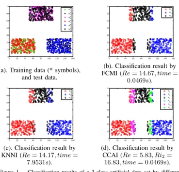
method5_{. The classification results of the test objects by}

different methods are given in Fig. 1-b–1-d. For notation

conciseness, we have denotedwte _,wtest_{, w}tr _,wtraining

and wi,...,k , wi ∪. . . ∪ wk. The error rate (in %) and

imprecision rate (in %) are specified in the caption of each subfigure. 0 20 40 60 80 100 120 140 160 0 10 20 30 40 50 60 70 w1 tr w2 tr w3 tr w1 te w2 te w3 te 0 20 40 60 80 100 120 140 160 0 10 20 30 40 50 60 70 w1 w2 w3

(a). Training data (* symbols), and test data.

(b). Classification result by FCMI (Re= 14.67, time= 0.0469s). 0 20 40 60 80 100 120 140 160 0 10 20 30 40 50 60 70 w1 w2 w3 0 20 40 60 80 100 120 140 160 0 10 20 30 40 50 60 70 w1 w2 w3 w1,2 w1,3 w2,3 (c). Classification result by KNNI (Re= 14.17, time= 7.9531s). (d). Classification result by CCAI (Re= 5.83, Ri2= 16.83, time= 0.0469s). Figure 1. Classification results of a 3-class artificial data set by different methods.

5_{In fact, the choice ofKranking from 7 to 15 does not affect seriously}

Because they value in the test sample is missing, the class

w3 appears partially overlapped with the classes w1 and w2

on their margins according to the value of x-coordinate as shown in Fig. 1-(a). The missing value of the samples in the overlapped parts can be filled by quite different estima-tions obtained from different classes with the almost same reliabilities. For example, the estimation of the missing values

of the objects in the right margin of w1 and the left margin

of w3 can be obtained according to the training class w1 or

w3. The edited pattern with the estimation from w1 will be

classified into classw1, whereas it will be committed to class

w3 if the estimation is drawn from w3. It is similar to the

test samples in the left margin of w2 and the right margin

of w3. This indicates that the missing value play a crucial

rule in the classification of these objects, but unfortunately the estimation of these involved missing values are quite uncertain according to context. So these objects are prudently classified

into the proper meta-class (e.g. w1∪w3 and w2∪w3) by

CCAI. The CCAI results indicate that these objects belong to one of the specific classes included in the meta-classes, but these specific classes cannot be clearly distinguished by the object based only on the available values. If one wants to get more precise and accurate classification results, one needs to request for additional resources for gathering more useful information. The other objects in the left margin of

w1, right margin of w2 and middle of w3 can be correctly

classified based on the only known value in x-coordinate, and it is not necessary to estimate the missing value for the classification of these objects in CCAI. However, all the test samples are classified into specific classes by the traditional methods KNNI and FCMI, and this causes many errors due to the limitation of probability framework. Thus, CCAI produces less error rate than KNNI and FCMI thanks to the use of meta-classes. Meanwhile, the computational time of CCAI is similar to that of FCMI, and is much shorter than KNNI because of the introduction of SOM technique in the estimation of missing values. It shows that the computational complexity of CCAI is relatively low. This simple example shows the interest and the potential of the credal classification obtained with CCAI method.

B. Experiment 2 (real data set)

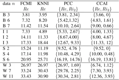
Four well known real data sets (Breast cancer, Iris, Seeds and Wine data sets) available from UCI Machine Learning Repository [31] are used in this experiment to evaluate the performance of CCAI with respect to KNNI, FCMI and PCC. ENN is also used here as standard classifier. The basic information of these four real data sets is given in Table I.

The cross validation is performed on all the data sets, and

we use the simplest 2-fold cross validation6 here, since it has

the advantage that the training and test sets are both large,

6_{More precisely, the samples in each class are randomly assigned to two}

setsS1 andS2having equal size. Then we train onS1and test onS2, and

reciprocally.

and each sample is used for both training and testing on each

fold. Each test sample has nmissing (unknown) values, and

they are missing completely at random in every dimension.

The average error rate Re and imprecision rateRi(for PCC

and CCAI) of the different methods are given in Table II. Particularly, the reported classification result of KNNI is the

average withK value ranging from 5 to 15.

Table I

BASIC INFORMATION OF THE USED DATA SETS.

name classes attributes instances

Breast (B) 2 9 699

Iris (I) 3 4 150

Seeds (S) 3 7 210

Wine (W) 3 13 178

Table II

CLASSIFICATION RESULTS FOR DIFFERENT REAL DATA SETS(IN%).

datan FCMI KNNI PCC CCAI

Re Re {Re, Ri2} {Re, Ri2} B 3 3.81 3.95 {3.81, 2.34} {3.66, 0} B 6 7.32 8.20 {5.42,1.32} {4.83, 1.61} B 7 11.42 11.54 {10.10, 2.64} {9.00, 0.66} I 1 7.33 4.89 {5.33, 2.67} {4.00, 1.33} I 2 14.11 11.33 {8.67,4.00} {8.00, 4.67} I 3 17.33 18.44 {12.67, 9.33} {11.33, 12} S 2 15.24 11.19 {9.52, 4.76 } {9.52, 0} S 4 17.14 11.98 {10.48, 4.29} {10.00, 0.48} S 6 20.95 25.71 {16.19, 14.76} {16.19, 13.81} W 3 26.97 26.97 {26.97, 1.69} {6.74, 1.12} W 7 33.24 30.43 {29.78, 2.25} {7.30, 3.93} W 11 33.43 30.90 {30.34, 2.81} {12.36, 3.93}

One can see that the credal classification of PCC and CCAI always produce the lower error rate than the traditional FCMI and KNNI methods, since some objects that cannot be correctly classified using only the available attribute values have been properly committed to the meta-classes, which can well reveal the imprecision of classification. In CCAI, some objects with the imputation of missing values are still classified into the meta-class. It indicates that these missing values play a crucial role in the classification, but the estimation of these missing values is no very good. In other words, the missing values can be filled with the similar reliabilities by different estimated data, which lead to distinct classification results. So we have to cautiously assign them to the meta-class to reduce the risk of misclassification. Compared with our previous method PCC, this new method CCAI generally provide better performance with lower error rate and imprecision rate, and it is mainly because more accurate estimation method (i.e.

SOM+KN N) for missing values is adopted in CCAI. This

shows the effectiveness and interest of this new CCAI method with respect to other methods.

V. CONCLUSION

A fast credal classification method with adaptive imputation of missing values (called CCAI) for dealing with incomplete pattern has been presented. In step 1 of CCAI method, some objects (incomplete pattern) are directly classified ignoring the missing values if the specific classification result can be ob-tained, which effectively reduces the computation complexity because it avoids the imputation of the missing values. How-ever, if the available information is not sufficient to achieve a specific classification of the object, we estimate (recover) the missing values before entering the classification procedure in the second step. The SOM and K-NN approaches are applied to make the estimation of missing attributes with a good compromise between the estimation accuracy and computation burden. Information fusion technique is employed to combine the multiple simple classification results respectively obtained from each training class for the final credal classification of object. The credal classification in this work allows the object to belong to different singleton classes and meta-class with different masses of belief. Once the object is committed to

a meta-class (e.g. A∪B), it means that the missing values

cannot be accurately recovered according to the context, and the estimation is not very good. Different estimations will lead

the object to distinct classes (e.g.AorB) involved in the

meta-class. So some other sources of information will be required to achieve more precise classification of the object if necessary. Two experiments have been applied to test the performance of CCAI method with artificial and real data sets. The results show that the credal classification is able to well capture the imprecision of classification and effectively reduces the misclassification errors as well.

REFERENCES

[1] P. Garcia-Laencina, J. Sancho-Gomez, A. Figueiras-Vidal, Pattern classification with missing data: a review, Neural Comput Appl. Vol.19:263–282, 2010.

[2] R.J. Little, D.B. Rubin,Statistical Analysis with Missing Data, John Wiley & Sons, New York, 1987 (Second edition published in 2002). [3] A. Farhangfar, L. Kurgan, J. Dy, Impact of imputation of missing

values on classification error for discrete data, Pattern Recognition Vol.41:3692–3705, 2008.

[4] D.J. Mundfrom, A. Whitcomb,Imputing missing values: The effect on the accuracy of classification, Multiple Linear Regression Viewpoints. Vol. 25(1):13–19, 1998.

[5] G. Batista, M.C. Monard, A Study of K-Nearest Neighbour as an Imputation Method, in Proc. of Second International Conference on Hybrid Intelligent Systems (IOS Press, v. 87), pp. 251–260, 2002. [6] J. Luengo, J.A. Saez, F.Herrera, Missing data imputation for fuzzy

rule-based classification systems, Soft Computing, Vol.16(5):863–881, 2012.

[7] D. Li, J.Deogun, W. Spaulding, B. Shuart,Towards missing data impu-tation: a study of fuzzy k-means clustering method, In: 4th international conference of rough sets and current trends in computing (RSCTC04), pp 573–579, 2004.

[8] Z. Ghahramani, M.I. Jordan,Supervised learning from incomplete data via an EM approach, In: Cowan JD et al. (Eds) Adv. Neural Inf. Process., Morgan Kaufmann Publishers Inc., Vol.6:120–127, 1994. [9] K. Pelckmans, J.D. Brabanter, J.A.K. Suykens, B.D. Moor,Handling

missing values in support vector machine classifiers, Neural Networks, Vol. 18(5-6):684–692, 2005.

[10] G. Shafer,A mathematical theory of evidence, Princeton Univ. Press, 1976.

[11] F. Smarandache, J. Dezert (Editors), Advances and applications of DSmT for information fusion, American Research Press, Rehoboth, Vol. 1-4, 2004-2015. http://fs.gallup.unm.edu/DSmT.htm

[12] P. Smets,The combination of evidence in the transferable belief model, IEEE Trans. on Pattern Anal. and Mach. Intell., Vol. 12(5):447– 458,1990.

[13] A.-L. Jousselme, C. Liu, D. Grenier, E. Boss´e,Measuring ambiguity in the evidence theory, IEEE Trans. on SMC, Part A: 36(5):890–903, Sept. 2006.

[14] T. Denœux, A k-nearest neighbor classification rule based on Dempster-Shafer Theory, IEEE Trans. on Systems, Man and Cyber-netics, Vol. 25(5):804–813, 1995.

[15] Z.-g. Liu, Q. Pan, J. Dezert, Gregoire MercierFuzzy-belief K-nearest neighbor classifier for uncertain data, in Proc. of 17th Int. Conference on Information Fusion (Fusion 2014), Spain, July 7-10, 2014. [16] Z.-g. Liu, Q. Pan, J. Dezert, G. Mercier, Credal classification rule

for uncertain data based on belief functions, Pattern Recognition, Vol. 47(7): 2532–2541,2014.

[17] T. Denœux, P. Smets,Classification using belief functions: relationship between case-based and model-based approaches, IEEE Trans. on Systems, Man and Cybernetics, Part B: Vol.36(6):1395–1406, 2006. [18] T. Denœux, A neural network classifier based on Dempster-Shafer

theory, IEEE Trans. Systems, Man and Cybernetics: Part A, Vol.30(2): 131–150, 2000.

[19] M.-H. Masson, T. Denœux,ECM: An evidential version of the fuzzy c-means algorithm, Pattern Recognition, Vol.41(4):1384–1397, 2008. [20] T. Denœux, M.-H. Masson,EVCLUS: EVidential CLUStering of

prox-imity data, IEEE Trans. on Systems, Man and Cybernetics: Part B, Vol.34(1):95–109, 2004.

[21] Z.-g. Liu, Q. Pan, J. Dezert, G. Mercier,Credal c-means clustering method based on belief functions, Knowledge-based systems, Vol.74: 119-132, 2015.

[22] T. Denœux,Maximum likelihood estimation from uncertain data in the belief function framework, IEEE Transactions on Knowledge and Data Engineering, Vol. 25(1):119–130, 2013.

[23] Z.-g. Liu, J. Dezert, Q. Pan, G. Mercier,Combination of sources of evidence with different discounting factors based on a new dissimilarity measure, Decision Support Systems, Vol.52:133–141, 2011.

[24] Z.-g. Liu, Q. Pan, G. Mercier, J. Dezert, A new incomplete pattern classification method based on evidential reasoning, IEEE Trans. Cybernetics, DOI:10.1109/TCYB.2014.2332037, 2014.

[25] T. Kohonen, The Self-Organizing Map, Proceedings of the IEEE, Vol.78(9):1464–1480, 1990.

[26] D. Dubois, H. Prade,Representation and combination of uncertainty with belief functions and possibility measures, Computational Intelli-gence, Vol. 4(4):244–264, 1988.

[27] J. Dezert, A. Tchamova, On the validity of Dempster’s fusion rule and its interpretation as a generalization of Bayesian fusion rule, International Journal of Intelligent Systems, Vol. 29(3):223–252, 2014. [28] F. Smarandache, J. Dezert, On the consistency of PCR6 with the averaging rule and its application to probability estimation, in Proc. of 16th Int. Conference on Information Fusion (Fusion 2013), Istanbul, Turkey, July 9-12, 2013.

[29] I. Hammami, J. Dezert, G. Mercier, A. Hamouda, On the estimation of mass functions using Self Organizing Maps, in Proc. of Belief 2014 Conf. Oxford, UK, Sept. 26–29, 2014.

[30] S. Geisser, Predictive inference: an introduction, New York, NY: Chapman and Hall, 1993.

[31] A. Frank, A. Asuncion,UCI machine learning repository, University of California, School of Information and Computer Science, Irvine, CA, USA, 2010. http://archive.ics.uci.edu/ml