04 August 2020
Band-Division vs. Space-Division Multiplexing: A Network Performance Statistical Assessment / Ferrari, A.; Virgillito, E.; Curri, V.. - In: JOURNAL OF LIGHTWAVE TECHNOLOGY. - ISSN 0733-8724. - ELETTRONICO. - 38:5(2020), pp. 1041-1049.
Original
Band-Division vs. Space-Division Multiplexing: A Network Performance Statistical Assessment
ieee Publisher: Published DOI:10.1109/JLT.2020.2970484 Terms of use: openAccess Publisher copyright
copyright 20xx IEEE. Personal use of this material is permitted. Permission from IEEE must be obtained for all other uses, in any current or future media, including reprinting/republishing this material for advertising or promotional purposes, creating .
(Article begins on next page)
This article is made available under terms and conditions as specified in the corresponding bibliographic description in the repository
Availability:
This version is available at: 11583/2827284 since: 2020-05-20T11:25:11Z
Band-division vs. Space-division multiplexing: a
Network Performance Statistical Assessment
Alessio Ferrari,
Student Member, IEEE,
Emanuele Virgillito,
Student Member, IEEE,
and Vittorio Curri,
Senior
Member, IEEE, Member, OSA
Abstract—We compare the networking merit of two possible multiplexing techniques on top of wavelength division mul-tiplexing to enlarge transmission capacity: the band division multiplexing (BDM) that aims at using up to all the U-to-O low-loss transmission bands available on the G-652.D fiber; and the spatial division multiplexing (SDM) implemented by activating additional fibers, used on the C-band only. We use the statistical network assessment (SNAP) to derive the networking performance as blocking probability vs. the total allocated traffic normalized with respect to the multiplexing cardinality. We analyze two network topologies: the German regional network and the US-NET continental network. In case dark fibers are available, SDM upgrades are always the best solution, enabling up to extra traffic of 12% and 17% at blocking probability equal to 10−3 on top of the multiplication by the multiplexing cardinality (NM) of 12, for the German and US-NET topology,
respectively. BDM solutions present worse performance, but mixed BDM/SDM solutions display quite limited penalties with respect to the pure SDM solution, up to the use of 16 THz per fiber. So, mixed BDM/SDM implementation seems the most convenient solution in case of limited availability of dark fibers. Pure BDM solutions occupying a bandwidth larger than 16 THz display an increasingly and considerable gap in the allocated traffic with respect to the pure BDM, so, their use must be considered only in case of total absence of available dark fibers.
Index Terms—Optical fiber networks, WDM networks, Optical fiber communication, Multi-band transmission, high-capacity systems
I. INTRODUCTION
T
HE 5G network revolution, together with the progres-sive and fast extension of cloud services and data-center interconnection, is driving a continuous growth in data-traffic demand, that will increasingly proceed during the next years [1]. Such an increased capacity request will first impact the optical backbone networks that will be requested to support a large increase in low-latency and high-capacity traffic, which will also considerably vary during the day. State-of-the-art transparent optical backbone networks deploy co-herent technologies for data transport and wavelength division multiplexing (WDM) on the fiber C-band. The traffic growth is already saturating the C-band for the deployed infrastructure in several regional networks. So, the operators are planning capacity upgrades, with the firm requirement of maximizing return on the capital expenditure (CAPEX), by minimizing the request for new equipment [2]. In case dark fibers are available, the most profitable solution for capacity upgrade isA. Ferrari, E. Virgillito and V. Curri are with the Dipartimento di Elet-tronica e Telecomunicazioni, Politecnico di Torino, Torino, Italy, e-mail: [email protected].
the deployment of new C-Band transmission lines by activating the available fibers duplicating transceivers, reconfigurable optical add-drop multiplexers (ROADMs) and amplifiers. Such an approach is the simplest implementation of the space-division multiplexing (SDM) [3], [4] on top of WDM, and it createsNSDMreplicas of the available lightpaths (LPs), where
NSDMis the SDM cardinality, i.e., the count of activated fibers.
In absence of available dark fibers, to avoid the deployment of new cables, the transmission upgrade can be addressed to the use of low-loss bands available in standard single-mode fibers (SSMF), beyond the C-band, by enlargingNBDM
times the occupied bandwidth, so implementing band-division multiplexing (BDM) [5]–[7] on top of WDM. The BDM may extend the exploited optical spectrum to the entire set of low-loss U-, L-, C-, S-, E- and O-band up to an overall transmission bandwidth of roughly ∼50 THz, in between 1360 nm and 1675 nm. In this case, the BDM cardinality (NBDM) indicates
how many times the bandwidth is enlarged from the C-band. In order to enable fair comparisons, we consider the C-band made of 80 channels only, contrary to the typical value of 96. We do not expect this hypothesis to modifying the generality of the outcomes. The BDM solution does not require installing new cables, while needs new transceivers, amplifiers and ROADM upgrades for the bands beyond the C-band. Network operators are already implementing the BDM solution by installing the commercially available C+L-band transmission lines. In the presented analysis, we suppose the availability of filters, transceivers, and amplifiers for all the low-loss bands. Not all of these components are yet commercially available, especially for the lumped amplifiers, but their feasibility has been extensively demonstrated [8]–[11]. Mixed SDM/BDM solutions can be considered in case of scarce availability of dark fibers. In case we consider to install new cables, the family of SDM implementations may include additional alternatives: multimode fibers (MMF), multicore fibers (MCF) and multiple parallel fiber (MPF) systems. In [4], [12]–[16], the SDM technologies have been extensively studied and compared from a propagation point-to-point physical layer perspective. Many studies have been carried out also from a networking perspective. In [17], the impact of spectral and spatial super-channel allocation policies is investigated in the context of SDM networks. In [18], the authors propose routing, space and spectrum allocation heuristics for SDM networks limiting the penalty of using joint switching and fractional joint switching. In [19], network performance of strongly coupled MCF and MPF are compared by investigating the switching techniques and fiber propagation performances.
chitecture for MCF flex-grid networks. Finally, in [21], the authors address the fundamentals of switching node design for WDM-SDM networks. In general, a transmission line using MMF or strongly coupled MCF may enable a larger capacity compared to MPF taking advantage of mitigating the nonlinear interference (NLI) [13], but they require complex super-MIMO transponders jointly operating on all cores/modes for each wavelength. Furthermore, as shown in [19], in a backbone network, MPF performs much better than strongly coupled MCFs, because of the strong networking penalty introduced by joint switching. Furthermore, we focus on the use of standard transceivers, thus, the best SDM implementation is the one based on MPF, as every coupling between cores induces a penalty, i.e., an excess disturbance caused by cross-talk among the cores. For this reason, we also skip weakly-coupled MCF technology. Hence, to fairly compare to BDM upgrades, in this article, we consider as SDM solution the MPF one. For the SDM implementation, we assume core continuity [20] within the ROADM, while for BDM we similarly consider wavelength continuity in ROADMs. This makes fair the comparison between SDM and BDM in terms of switching matrix complexity at the ROADM node. Moreover, as shown in [19], by removing the core continuity constraints network performance is not significantly enhanced. Furthermore, we assume wavelength continuity as we do not consider the use wavelength converters.
For both BDM and SDM implementations, we suppose to operate onto the SSMF with reduced water-peak – the ITU-T G.652.D fiber type [22]–, as it is the most deployed fiber type [23]–[25] and it has the wider single-mode, low-loss, and non-zero dispersion bandwidth, among the largely installed fiber types. The studies presented in [5], [6] investigate the point-to-point performance of a BDM transmission line, while the networking performance of BDM has not yet been in-vestigated. To properly consider the multiband propagation impairments, in [6], we show the importance of including the stimulated Raman scattering (SRS) while evaluating the quality of transmission (QoT) given by the generalized signal-to-noise ratio (GSNR) including both the accumulation of ASE noise and nonlinear interference (NLI) [26]. This is necessary because the SRS modifies the fiber gain/loss profile due to power transfer from higher to lower frequencies which becomes maximally intense in case the frequency offset is roughly 13 THz. This SRS-induced spectral tilt modifies the amplified spontaneous emission (ASE) noise accumulation that becomes dominant in spectral areas that are strongly depleted by the SRS – the higher-frequency bands – and enables a larger generation of nonlinear interference (NLI) on bands experiencing a larger SRS-induced power transfer – the lower-frequency bands. The generalized Gaussian noise (GGN) model [27] has been proposed to include SRS when computing the fiber nonlinear interference (NLI) [28], [29]. In this work, we assess the overall network capacity versus blocking probability (BP) considering several combinations of BDM and SDM upgrades by using the statistical network assessment process (SNAP) [30]–[32] including the physical layer awareness. To this aim, SNAP considers a network
where graph nodes are ROADM network nodes and graph edges are the optical transmission lines, whose weight is the GSNR degradation per wavelength, as shown in [33]. By implementing a multiplexing upgrade, the graph is replicated
NM times, with proper weights on edges. Relying on this
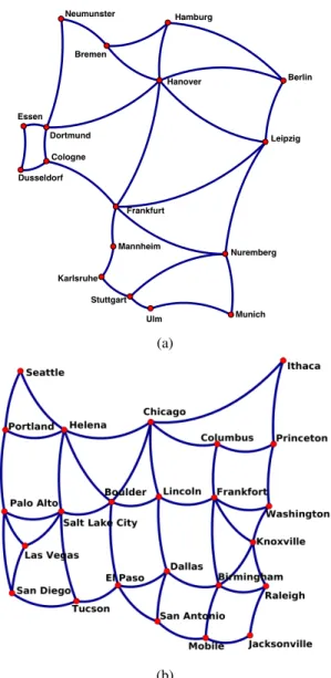
network abstraction, Monte-Carlo analyses on traffic load are performed by the SNAP framework and the average blocking probability vs. the allocated traffic is obtained for the inves-tigated scenarios, so, enabling a networking comparison of different solutions. SNAP is applied to the German network and the US-NET network topologies that are depicted in Fig. 2a and Fig. 2b, respectively.
BDM upgrades explore the progressive enlargement of the occupied bandwidth from the C-band only (4 THz), up to the U, L, C, S, E and O bands (∼50 THz). On the contrary, SDM upgrades enlarge the number of parallel fibers used, using only the C-band. We compare multiplexing upgrades by exploiting pure BDM, pure SDM, and mixed solutions, progressively increasing the multiplexing cardinality (NM), i.e., a
multiplica-tive factor giving the total number of wavelengths times the number of parallel fibers, with respect to the single-fiber, C-Band only case. We evaluate the BP vs total allocated traffic normalized to theNM. In this paper, we investigate the trends
of BDM/SDM solutions by considering also mixed cases in two network topologies and comparing them with respect to a reference in order to investigate relative benefits. This leads to an assessment on the bands that can be effectively used and on the ones limiting the overall supported traffic, at a given BP.
The article is organized as follows. Sec. II describes in detail the methodology adopted by addressing how the physical layer is abstracted and how the LP GSNR is computed, how the network resource allocation process is managed and how the networking performance is computed. Then, Sec. III presents the scenarios under analysis by describing the optical param-eters, the system configuration, and the considered networks. Afterward, Sec. IV shows the numerical results in terms of BP vs the allocated traffic normalized to the multiplexing cardinality. Focusing on the performance at BP= 10−3, or lower, the main results display that an L+C+S system presents negligible traffic reduction with respect to the SDM solution with a cardinality of three. Furthermore, even if the pure SDM upgrades always perform better than the BDM and mixed BDM/SDM, the advantage of SDM solutions is roughly limited to 20% when 16 THz L+C+S bands for BDM are used. Finally, Sec. V draws the final comments and conclusions.
II. METHODOLOGY
In our analysis, we upgrade spatial and spectral resources which are quantified by their cardinality: the SDM cardinality is the number of parallel fibers used, while the BDM cardinal-ity is the enlargement factor in the occupied bandwidth with respect to a 80 channel C-Band scenario, that is the reference scenario. Thus, the total number of WDM channels per fiber (Nλ) is
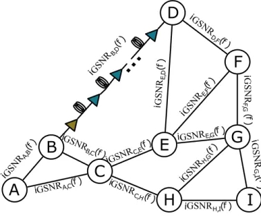
A
E
B
D
H
C
G
I
F
B,D( ) f GSNR E,G( )f GSNR E,F( ) f GSNR E, D () f GSNR B,C( )f GSNR A,B( ) f GSNR A,C( )f GSNR C,H ( )f GSNR C,E( )f GSNR D,F( )f GSNR F,G ( )f GSNR G ,I( )f GSNR H,I( )f GSNR H,G ( ) GSNR f i i i i i i i i i i i i i iFig. 1: Abstraction of the physical layer.
The network physical layer is abstracted according to the waveplane model [34]: resources are mapped in a number of parallel waveplanes equal to NSDM ×Nλ; each waveplane
is one spatial and spectral resource in the network. Each waveplane contains a weighted graph abstracting the physical layer as depicted in Fig. 1. The graph nodes are the ROADM nodes and each graph edge is a transmission line connecting two ROADM nodes including pre-amp and booster amplifiers. Each edge is characterized by a value of GSNR degradation (iGSNR(fi)l,m) representing the QoT degradation introduced by each transmission line between node l and node m for the i-th channel at the frequency fi. The GSNR takes into
account the SRS, the NLI and the ASE noise. Thus, it neglects other impairments such as filtering effects and non-ideality of the components leading to frequency dependent penalties. iGSNR(fi)l,m does not depend on the deployed
spatial resource, but only on the spectral one, being a function of fi, since all the parallel fibers have the same performance.
The iGSNR(fi)l,mof a transmission line is determined by the SNR degradation introduced by each network element as:
iGSNR(fi)l,m=iOSNRBST(fi)+ Ns X n=1 (iSNRNLn(fi) +iOSNRn(fi)) , (2)
where, iOSNRBST(fi)is the OSNR degradation introduced by
the booster amplifier, and iSNRNLn(fi) and iOSNRn(fi) are
the ones introduced by the n-th fiber span and by the n-th amplifier respectively. NS is the number of spans making the
transmission line.
The iOSNR of each amplifier is iOSNRn(fi) = PASE(fi)
Ps(fi)G(fi), (3)
where Ps(fi) is the i-th signal power at the input of the amplifier, G(fi) is the amplifier gain at fi and PASE(fi) is
the ASE noise power. For the booster amplifier, Ps(fi) is
equal to the transmitted powerPTX(fi).PASE(fi)is computed
according to the formula
PASE(fi) =F(fi)hfi(G(fi) + 1)Bref. (4)
F(fi) is the amplifier noise figure, his the Planck constant andBref is the reference bandwidth which is set to the signal
symbol rateRs. The iSNRNL value of each fiber span is
iSNRNLn(fi) =
PNLI(fi)
Ps(fi)LF(fi)
, (5)
where Ps(fi) is the power of the i-th channel at the input of the fiber, LF(fi) is the fiber attenuation including any
SRS effect and PNLI(fi) is the NLI power in a reference
bandwidth equal to the signal symbol rate. The impact of SRS on fiber propagation is evaluated according to the SRS equations [35], while PNLI(fi) is computed according to the
GGN-model assuming a locally white NLI power spectral density and full spectral load as shown in [27], [36]. In our analysis, we assume to rely on lumped amplification or on Raman amplification in moderate pumping regime, that can be assumed as lumped for propagation effects [37]. As for any other components, also for the amplifiers, the presented analysis deliberately does not include implementation issues, to keep the target comparison as general as possible. So, we do not consider any ripple in the gain and the noise. We only diversify amplification on different bands by considering different values of noise figure (NF). NFs are to be intended as equivalent noise figures including the losses of multiplexers, demultiplexers and couplers. The transmitted powerPTX(fi)
and the gain of each amplifier are set according to a per-band local-optimization global-optimization (LOGO) approach [38], [39]. This waveplane structure is used to evaluate the GSNR of a LP by accumulating the GSNR degradation of each transmission line along a path as:
GSNR(fi) = X (l,m)∈LP iGSNR(fi)l,m −1 . (6)
The node pair(l, m)indicates each transmission line between the node l and the node m, along the path. Based on the GSNR of a LP, the feasible data rate is evaluated assuming a flexible transceiver capable of achieving a close to Shannon spectral efficiency based on the GSNR of the LP at the price of an overhead. The waveplanes are also used to manage the resource allocation in the routing, wavelength and spatial assignment (RWSA) process which works as follows: for each connection request between a source and a destination node,k
paths are computed according to ak-shortest path algorithm. Then, starting from the shortest path, resource availability is verified in each waveplane along the path. If several resources are available, the one providing the highest GSNR is deployed. Otherwise, if there are not available resources to deploy the shortest path, the 2-nd shortest path is attempted to be allocated. The process goes on as long as the demand is not allocated or all the paths and waveplanes are attempted. This algorithm does not guarantee an optimum use of the network resources but provides just the better resource among the available ones to the traffic request at the time it occurs.
SNAP [30], [31] by progressively loading the network with random realizations of traffic demands according to a con-nectivity matrix and to a given probability distribution of connection requests. Thus, by recording each acceptance and blocking event of each traffic request, and by combining this information with the feasible data rate on each deployed LP, we can evaluate the progressive increase of the blocking probability while the total allocated traffic grows, for each Monte Carlo run. Finally, a unique blocking probability vs total allocated traffic curve is obtained by averaging among the different Monte Carlo realizations. The SNAP method is then applied to both the considered networks and to each combination of NBDM and NSDM to obtain a set of fairly
comparable results. A fair comparison needs to compare upgrades with the same multiplexing cardinality defined as
NM=NSDM×NBDM. (7)
To estimate the gain/loss of each configuration as normalized total allocated traffic at a given blocking probability, we consider the reference scenario NM = NBDM =NSDM = 1,
i.e., the single-fiber, C-band only, transmission line. III. ANALYSIS
We investigate several multiplexing upgrades grouped by
NM equal to 1, 2, 3, 4, 6 and 12. Then, all the combinations
of NBDM andNSDM matching the values ofNM are explored.
The description of the analyzed multiplexing upgrades is sum-marized in Tab. II. Also, the NM= 1scenario is investigated
to assess the reference perfomance. The investigated solutions are classified into four categories:
1) Reference scenario in whichNSDM= 1andNBDM= 1
2) Pure BDM, when NSDM= 1andNBDM=NM
3) Pure SDM, whenNBDM= 1 andNSDM=NM
4) Mixed upgrades in which NSDM6= 1 andNBDM6= 1
Tab. III displays the total number of available spectral slots
Nλ, the bandwidth occupation of such slots in the U, L, C,
S, E, O-bands and the total available bandwidth as NBDM
increases.
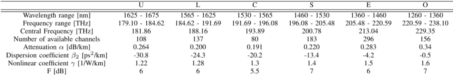
As previously stated, we suppose to rely on elastic transceivers operated using polarization-multiplexed coherent technologies at the symbol rate of 32 GBaud. We suppose to exploit the fixed grid WDM technology in the ITU-T 50 GHz WDM grid, thus enabling transmission up to 80 channels for each considered 4 THz spectral slot. The amplified transmis-sion lines are supposed to be uniformly made of SSMF, as in the G.652.D ITU-T recommendation. The distance between amplifier sites is supposed to be constant on the entire network for both the considered topologies and set to 75 km. Tab. I summarizes the fiber propagation parameters at the central frequency of each considered transmission band. In particular, it shows the attenuation (α), the chromatic dispersion param-eter (β2) and the nonlinear coefficient (γ). To recover losses,
channels on each optical band (U-, L-, C-, S-, E- and O-band) are amplified by in-line lumped amplification. As already stated, it is out of the scope of this analysis to analyze in detail the available and feasible technologies for multi-band network
Berlin Bremen Dortmund Dusseldorf Essen Frankfurt Hanover Karlsruhe Cologne Leipzig Mannheim Munich Nuremberg Stuttgart Ulm (a) (b)
Fig. 2: Analyzed networks: German (a) and US-NET (b) topologies.
operation, so, to differentiate the amplification performance on different band, we only considered different noise figures, according to the literature results [8]–[11]. The considered noise figures values in the analyzed bands are reported in Tab. I. Each amplifier is supposed to provide flat gain and noise figure, while, we suppose a cascaded gain flattening filter (GFF) compensating for the spectral modifications introduced by the SRS [40]. Hence, a flat spectrum per band is used at the input of each fiber span, while the power level per band is set according to the LOGO strategy [38], [39]. Pre-tilt strategies can also be used to further improve the channel capacity for both BDM and SDM [41], by performing case-by-caseoptimizations, that are out of the scope of the presented analysis. In general, we do not expect a substantial change in the outcomes of the compared analysis of BDM and SDM by using specific optimizations.
We applied the described analysis to two network topolo-gies: the German topology shown in Fig. 2a that is a wide re-gional network, and the US-NET topology depicted in Fig. 2b that is a wide continental network. The German topology has
TABLE I: Per band parameters
U L C S E O
Wavelength range [nm] 1625 - 1675 1565 - 1625 1530 - 1565 1460 - 1530 1360 - 1460 1260 - 1360 Frequency range [THz] 179.10 - 184.62 184.62 - 191.69 191.69 - 196.08 196.08 - 205.48 205.48 - 220.59 220.59 - 238.10
Central Frequency [THz] 181.86 188.16 193.89 200.78 213.04 229.35
Number of available channels 108 137 80 183 296 156
Attenuationα[dB/km] 0.264 0.200 0.191 0.220 0.283 0.34
Dispersion coefficientβ2[ps2/km] -30.8 -24.3 -20.2 -13.4 -4.2 -0.5
Nonlinear coefficientγ[1/W/km] 1.22 1.28 1.3 1.4 1.5 1.6
F [dB] 6 6 5.5 7 6 7
TABLE II:NM,NBDM andNSDM of each investigated upgrades.
Pure BDM Mixed Upgrades Pure SDM
NM NBDM NSDM NBDM NSDM NBDM NSDM NBDM NSDM NBDM NSDM NBDM NSDM 2 2 1 - - - 1 2 3 3 1 - - - 1 3 4 4 1 2 2 - - - 1 4 6 6 1 3 2 2 3 - - - - 1 6 12 12 1 6 2 4 3 3 4 2 6 1 12
TABLE III: BDM bandwidth occupation
Number of channels per band Total
NBDM Nλ U L C S E O Bandwidth 1 80 - - 80 - - - 4 THz 2 160 - 80 80 - - - 8 THz 3 240 - 137 80 23 - - 12 THz 4 320 - 137 80 103 - - 16 THz 6 480 80 137 80 183 - - 24 THz 12 960 108 137 80 183 296 156 48 THz
17 nodes and 26 edges, and the average distance between two ROADM nodes is 207 km for an overall covered area with a diameter of 600 km and an average node degree of 3.1. Instead, the US-NET topology has 24 nodes and 44 edges and the average distance between ROADM nodes is 308 km for a covered area with a diameter of4 000km and an average node degree of 3.6. The two topologies have similar node degrees even if they present different covered areas. The connection requests are generated by assuming any-to-any connectivity with a uniform probability distribution. The requests are allocated according to the k-shortest-path RWSA algorithm previously described which computesk= 15paths per source-destination pair. We exploit the SNAP [30], [31] framework with progressive traffic load, so, for all the considered scenar-ios, the two network topologies are loaded withNM Cdifferent
traffic random realizations of the connection requests up to the saturation to derive the average merit parameter that is the blocking probability vs the overall traffic. For the considered scenarios, after a convergence test, we setNM C = 7500. Then,
we evaluate the BP and the total allocated traffic per MUX cardinality, i.e., the overall allocated traffic in the network normalized with respect to NM, to fairly compare all the
scenarios. We also evaluate themultiplexing gain/lossin terms of percentage of the overall allocated normalized traffic for an upgrade solution with respect to the single-fiber/single-band scenario NM = 1. Such evaluation enables a fair ranking of
the explored multiplexing scenarios.
IV. RESULTS
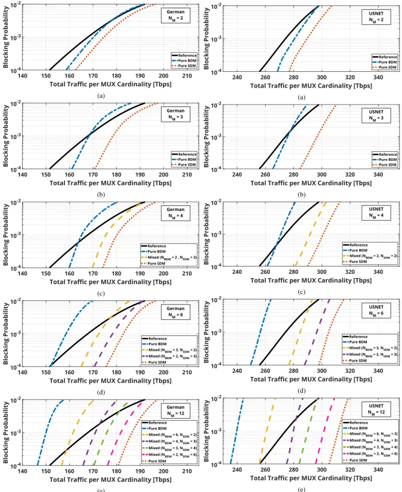
The outcomes of the SNAP analyses are the average BP vs the overall allocated traffic normalized with respect to the multiplexing cardinality. The plots of these results are depicted in Fig. 3 and Fig. 4, for the German and US-NET topologies, respectively. Sub-figures refer to the explored multiplexing cardinalities:NM= 2,3,4,6,12. Every plot displays the
refer-ence scenario as solid black lines, the pure SDM multiplexing solutions as dash-dotted blue lines, the pure BDM multiplexing upgrades as dotted red lines and the mixed upgrades as dashed lines. ForNM = 2(Fig. 3a and Fig. 4a), both pure BDM and
pure SDM upgrades present a multiplexing gain compared to the reference. As expected, pure SDM performs better than the reference, because a larger multiplexing cardinality introduces network flexibility, so reducing the number of blocking events per fiber. Also, BDM displays better performance than the reference, because the larger number of available LP per fiber increases the network flexibility as well as the increase in the number of fibers. However, BDM does not perform as well as SDM, because of the poorer QoT caused by the deployment of a larger number of channels in a single fiber. Already with NM = 2, BP vs normalized traffic are steeper
for BDM and SDM with respect to the reference scenario: this is caused by the improved network flexibility enabled by the increase of multiplexing cardinality that is larger at lower BP and decreases when the BP increases. Furthermore, curves referred to pure BDM and pure SDM are practically parallel, as both enable network flexibility, and the gap is due to the poorer BDM transmission performance. When a multiplexing technique with cardinality of two is applied, the behavior of the two network topologies is qualitatively very similar, mostly because the node degree is similar. However, the overall normalized traffic allocated on the US-NET is larger because of the larger number of nodes and transmission lines dominating the performance with respect to the longest propagation distances.
Then, by enlarging NM to 3 (Fig. 3b and Fig. 4b) and
to 4 (Fig. 3c and Fig. 4c), results evolve according to the behavior observed for NM = 2. Pure SDM is always the
140 150 160 170 180 190 200 210 Total Traffic per MUX Cardinality [Tbps] 10-4 10-3 Blocking Probability Reference Pure BDM Pure SDM German NM = 2 (a) 140 150 160 170 180 190 200 210
Total Traffic per MUX Cardinality [Tbps] 10-4 10-3 10-2 Blocking Probability Reference Pure BDM Pure SDM German NM = 3 (b) 140 150 160 170 180 190 200 210
Total Traffic per MUX Cardinality [Tbps] 10-4 10-3 10-2 Blocking Probability Reference Pure SDM German NM = 4 Pure BDM Mixed (NBDM = 2 , NSDM = 2) (c) 140 150 160 170 180 190 200 210
Total Traffic per MUX Cardinality [Tbps]
10-4 10-3 10-2 Blocking Probability Reference Pure BDM Pure SDM German NM = 6 Mixed (NBDM = 3, NSDM = 2) Mixed (NBDM = 2, NSDM = 3) (d) 140 150 160 170 180 190 200 210 Total Traffic per MUX Cardinality [Tbps] 10-4 10-3 10-2 Blocking Probability Reference Mixed (NBDM = 3, NSDM = 4) Mixed (NBDM = 2, NSDM = 6) Pure SDM German NM = 12 Pure BDM Mixed (NBDM = 6, NSDM = 2) Mixed (NBDM = 4, NSDM = 3) (e)
Fig. 3: Network performances in the German topology by varying the multiplexing cardinalityNM: 2 (a), 3 (b), 4 (c), 6
(d) and 12 (e).
240 260 280 300 320 340
Total Traffic per MUX Cardinality [Tbps]
10-4 10-3 10 Blocking Probability Reference Pure BDM Pure SDM USNET NM = 2 (a) 240 260 280 300 320 340
Total Traffic per MUX Cardinality [Tbps]
10-4 10-3 10-2 Blocking Probability Reference Pure BDM Pure SDM USNET NM = 3 (b) 240 260 280 300 320 340
Total Traffic per MUX Cardinality [Tbps]
10-4 10-3 10-2 Blocking Probability Reference Pure SDM USNET NM = 4 Pure BDM Mixed (NBDM = 2, NSDM = 2) (c) 240 260 280 300 320 340
Total Traffic per MUX Cardinality [Tbps]
10-4 10-3 10-2 Blocking Probability Reference Pure SDM USNET NM = 6 Pure BDM Mixed (NBDM = 3, NSDM = 2) Mixed (NBDM = 2, NSDM = 3) (d) 240 260 280 300 320 340
Total Traffic per MUX Cardinality [Tbps] 10-4 10-3 10-2 Blocking Probability Reference Pure BDM Mixed (NBDM = 6, NSDM = 2) Mixed (NBDM = 4, NSDM = 3) Mixed (NBDM = 3, NSDM = 4) Mixed (NBDM = 2, NSDM = 6) Pure SDM USNET NM = 12 (e)
Fig. 4: Network performances in the US-NET topology by varying the multiplexing cardinalityNM: 2 (a), 3 (b), 4 (c), 6
140 150 160 170 180 190 Ref eren ce Pur e BDM Pu re SDM Pur e BDM Pur e SDM Pur e BDM Pu re SDM Pur e BDM Pur e SDM Pur e BDM Pur e SDM M ixed (NBDM = 2, NSDM = 2) NM= 1 M ixed (NBDM = 3, NSDM = 2) M ixed (NBDM = 2, NSDM = 3) M ixed (NBDM = 6, NSDM = 2) M ixed (NBDM = 4, NSDM = 3) M ixed (NBDM = 3, NSDM = 4) M ixed (NBDM = 2, NSDM = 6) NM= 2 NM= 3 NM= 4 NM= 6 NM= 12 Total Tra ffi c per MUX Cardinality [Tbp s] German (a) 200 220 240 260 280 300 320 Ref eren ce Pur e BDM Pu re SDM Pur e BDM Pur e SDM Pur e BDM Pu re SDM Pur e BDM Pur e SDM Pur e BDM Pur e SDM NM= 1 NM= 2 NM= 3 NM= 4 NM= 6 NM= 12 M ixed (NBDM = 2, NSDM = 2) M ixed (NBDM = 3, NSDM = 2) M ixed (NBDM = 2, NSDM = 3) M ixed (NBDM = 6, NSDM = 2) M ixed (NBDM = 4, NSDM = 3) M ixed (NBDM = 3, NSDM = 4) M ixed (NBDM = 2, NSDM = 6) Total Tra ffi c per MUX Cardinality [Tbp s] USNET (b)
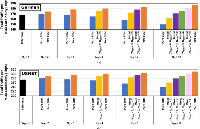
Fig. 5: Total traffic per MUX cardinality at BP10−3 in German (a) and US-NET (b) topologies.
best solution, as it does not impair transmission performance while enlarging the multiplexing cardinality. Moreover, the low-BP performance per fiber increases with the cardinality, since the network flexibility keeps improving. As expected, as cardinality increase, the pure BDM curves are parallel to the pure SDM, but the gap gets larger since the BDM QoT gets progressively worse. Mixed solutions fall in between with similar trends and gaps determined by the transmission performance. Even at larger multiplexing cardinalities the two topologies show similar trends, but curves of BP vs traffic are steeper for the larger-scale US-NET topology. This is due to the larger traffic allocation with respect to the reference at low BP. However, as the network gets loaded, i.e. at larger BPs, the traffic allocation slows down due to saturation effects happening between BP =10−3and BP =10−2for the
smaller-size German topology, and for BP larger than 10−2 for the
wider US-NET topology. For BP =10−4, pure BDM upgrades
present a multiplexing gain of 6% in the German network and up to 4% for the US-NET network while, for BP =10−2, the
multiplexing loss is within 5% for both the topologies. Results for larger NM of 6 and 12 are displayed in Fig. 3d
and Fig. 3e, and in Fig. 4d and Fig. 4e, for the German and US-NET topology, respectively. Qualitatively, the behavior is very similar to the one observed at lower cardinality: pure SDM is the best performing solution, while BDM is the
opposite, with a gap increasing with the cardinality since BDM must turn-on the fiber transmission bands with limited transmission performance while NM grows. Mixed solutions
fall in between, showing that BDM is giving limited trans-mission penalty up to the use of 16 THz. On one hand, pure SDM upgrades yield a multiplexing gain up to 17% and 16% when NM = 6 for the German network and the
US-NET topology, respectively, which increases up to 20% for both the topologies for NM = 12. On the other hand,
the pure BDM leads to a multiplexing loss, although limited to 12% and a 10% for the German and US-NET topology, respectively, when NM= 6. This capacity loss of pure BDM
solutions grows considerably when 48 THz per fiber is used (NBDM = 12) and goes up to 18% for both the topologies,
due to the low transmission performance of the used bands, mainly in the O-band. Mixed solutions display intermediate behaviors, showing that implementing BDM up toNBDM= 4
is always inducing penalty limited to 2% with respect to the pure BDM, introducing beneficial network flexibility. For all the analyzed multiplexing upgrades, the two topologies show very similar behaviors in the multiplexing gain/loss even if their geographical extension is quite different. Specifically, the hierarchy of solutions is kept, and the main difference is in the total normalized traffic that is larger on the US-NET because of the larger availability of transmission resources. So, we
medium-to-large scale backbone networks with node degrees large enough to limit the blocking in ROADM nodes.
The results showed before are summarized as total nor-malized traffic at a given BP. The total traffic per MUX cardinality at BP = 10−3 for the German network and the US-NET network are reported in Fig. 5a and in Fig. 5b, respectively. Pure SDM shows, for both the topologies, an initial capacity growth with respect to the reference scenario of roughly 5% for NM= 2, which increases to 7%, 8%, and
10% when NM = 3, NM = 4 and NM = 6, respectively.
This extra gain is due to excess network flexibility introduced by the increase of NM, while transmission performance does
not degrade due to the use of separate fibers. For NM = 12,
performance gain with respect to pure SDM for the two topologies diverges, being 12% for the German network and 17% in the US-NET network. This difference is due to the larger average node degree of the US-NET network which enables larger network flexibility while NM grows. For both
the topologies, the normalized traffic per MUX cardinality of pure BDM shows an initial multiplexing gain of 2% for
NM = 2, which reduces to almost 0% for NM equal to 3
and 4. So, up to NM = 4, network flexibility counteracts
transmission penalties. ForNM larger than 4, instead, the pure
BDM solutions display a capacity loss of 6% for NBDM= 6,
for both topologies, because the poor QoT now dominates the performance despite of the achieved network flexibility. So, BDM seems to be a very good solution to increase network capacity up to a multiplexing cardinality of 4, while, for larger cardinality, it seems convenient to activate also additional fibers, if available. Hence, implementing mixed SDM/BDM solutions, performance of mixed upgrades is bounded between pure SDM gain – up to 17% - and pure BDM loss – less than 9%.
V. CONCLUSION
We investigated network performance enabled by different choices of multiplexing upgrades. We compared two opposite multiplexing solutions: the band division multiplexing aimed at extending the transmission capacity by activating the avail-able low loss bands in G.652.D fibers up to 50 THz and the SDM technique based on C-band transmission over several parallel fibers. Pure BDM is the only solution when additional fibers are not available, while pure SDM needs to activate a number of fibers equal to the target multiplexing cardinality. To keep the analysis as general as possible, we did not consider per channel any spectral optimization as well as components’ peculiarities on different bands. So, the total capacity may be further improved but, we do not expect major changes in BDM vs SDM relative results thus, we expect to depict a general BDM vs SDM comparison.
We compared several network upgrades by enlarging the occupied bandwidth up to 50 THz – pure BDM solution with NM = 12 – and by increasing the number of parallel
fibers used up to 12 – pure SDM solution with NM = 12.
We also analyzed mixed BDM/SDM solutions. We used the SNAP framework to derive network performance as blocking
respect to the multiplexing cardinality. We analyzed two network topologies: the German large regional topology and the large US-NET continental topology. For both topologies, the implementation of multiplexing enables network flexibility that increases with the multiplexing cardinality, independently of the chosen multiplexing technology. It enables a larger traffic allocation with respect to the reference case, at limited BP that reduces with the BP increase, because of saturation effects happening between BP = 10−3 and BP = 10−2 for the smaller German topology, and for BP larger than 10−2
for the wider US-NET topology. All the analyzed solutions show very similar behavior, and the BP vs traffic curves are almost parallel for each topology, given the multiplexing cardinality. This is because the behavior is determined by the network flexibility, while capacity gaps are induced by poorer transmission performance of the BDM solutions.
The best solution is always the pure SDM, which enables a performance gain with respect to the reference of 12% for the German topology and of 17% for the US-NET topology at BP = 10−3, for N
M = 12. This means that besides
the NM-plication of traffic enabled by multiplexing, extra
traffic of 12% and 17% is enabled by the network flexibility, on the German and US-NET topology, respectively. On the contrary, BDM solutions rely on progressively lower QoT as the multiplexing cardinality grows. So, pure BDM upgrades show limited capacity gain with respect to the reference only up toNM = 4, then, for largerNM, BDM induces a capacity
loss that increases up to 9%, at BP=10−3, forN
M = 12, for
both the German network and the US-NET network.
So, in general, when dark fibers are available, the pure SDM solution is always convenient, otherwise mixed BDM/SDM solutions are excellent compromises if limiting the use of BDM to up to 16 THz. These mixed solutions show a very limited penalty with respect to the pure SDM solution, at BP = 10−3, for both the considered topologies. For larger
cardinalities, the use of BDM induces a larger penalty, so, it seems to be a feasible solution only when dark fibers are absent.
The two analyzed network topologies, show very similar behavior, so the presented results can be qualitatively extended to all network topologies with considerable fiber propagation. The absence of significant propagation, in fact, would make the BDM identical to SDM in terms of performance.
REFERENCES
[1] V. N. I. Cisco, “Vni global fixed and mobile internet traffic fore-casts,” https://www.cisco.com/c/en/us/solutions/service-provider/visual-networking-index-vni/index.html, 2014.
[2] G. Wellbrock and T. J. Xia, “How will optical transport deal with future network traffic growth?” in2014 The European Conference on Optical
Communication (ECOC). IEEE, sep 2014.
[3] P. J. Winzer, “Optical networking beyond wdm,” IEEE Photonics Journal, vol. 4, no. 2, pp. 647–651, 2012.
[4] R.-J. Essiambre and R. W. Tkach, “Capacity trends and limits of optical communication networks,”Proceedings of the IEEE, vol. 100, no. 5, pp. 1035–1055, 2012.
[5] J. K. Fischer, M. Cantono, V. Curri, R.-P. Braun, N. Costa, J. Pedro, E. Pincemin, P. Doar´e, C. Le Bou¨ett´e, and A. Napoli, “Maximizing the capacity of installed optical fiber infrastructure via wideband transmis-sion,” in 2018 20th International Conference on Transparent Optical
[6] A. Ferrari, A. Napoli, J. K. Fischer, N. Costa, A. D’Amico, J. Pedro, W. Forysiak, E. Pincemin, A. Lord, A. Stavdas, J. P. F.-P. Gimenez, G. Roelkens, N. Calabretta, S. Abrate, B. Sommerkorn-Krombholz, and V. Curri, “The achievable capacity of multi-band transmission systems using itu-t g.652.d optical fibers,”Submitted to JLT.
[7] A. Ferrari, A. Napoli, J. K. Fischer, N. Costa, J. a. Pedro, N. Sambo, E. Pincemin, B. Sommerkohrn-Krombholz, and C. Vittorio, “Upgrade capacity scenarios enabled by multi-band optical systems,”ICTON 2019. [8] Fiberlabs-Inc, “Praseodymium fluoride fiber glass doped amplifier,”
www.fiberlabs.com. [Online]. Available: www.fiberlabs.com
[9] E. Dianov, “Bismuth-doped optical fibers: a challenging active medium for near-IR lasers and optical amplifiers,”Light: Science & Applications, vol. 1, 2012.
[10] S. Aozasaet al., “Tm-doped fiber amplifiers for 1470-nm-band WDM signals,”PTL, vol. 12, no. 10, pp. 1331–1333, 2000.
[11] D. Chestnut, C. de Matos, P. Reeves-Hall, and J. Taylor, “Co-and counter-propagating second-order-pumped lumped fiber raman ampli-fiers,” inOptical Fiber Communication Conference. Optical Society of America, 2002, p. ThB2.
[12] R. Ryf, J. C. Alvarado, B. Huang, J. Antonio-Lopez, S. H. Chang, N. K. Fontaine, H. Chen, R.-J. Essiambre, E. Burrows, R. Amezcua-Correa et al., “Long-distance transmission over coupled-core multicore fiber,”
in ECOC 2016-Post Deadline Paper; 42nd European Conference on
Optical Communication. VDE, 2016, pp. 1–3.
[13] C. Antonelli, M. Shtaif, and A. Mecozzi, “Modeling of nonlinear prop-agation in space-division multiplexed fiber-optic transmission,”Journal of Lightwave Technology, vol. 34, no. 1, pp. 36–54, 2016.
[14] S. Matsuo, K. Takenaga, Y. Sasaki, Y. Amma, S. Saito, K. Saitoh, T. Matsui, K. Nakajima, T. Mizuno, H. Takaraet al., “High-spatial-multiplicity multicore fibers for future dense space-division-multiplexing systems,”Journal of Lightwave Technology, vol. 34, no. 6, pp. 1464– 1475, 2016.
[15] T. Hayashi, T. Sasaki, and E. Sasaoka, “Multi-core fibers for high capacity transmission,” inOFC/NFOEC. IEEE, 2012, pp. 1–3. [16] T. Hayashi, T. Taru, O. Shimakawa, T. Sasaki, and E. Sasaoka, “Design
and fabrication of ultra-low crosstalk and low-loss multi-core fiber,” Optics express, vol. 19, no. 17, pp. 16 576–16 592, 2011.
[17] P. S. Khodashenas, J. M. Rivas-Moscoso, D. Siracusa, F. Pederzolli, B. Shariati, D. Klonidis, E. Salvadori, and I. Tomkos, “Comparison of spectral and spatial super-channel allocation schemes for sdm networks,” Journal of Lightwave Technology, vol. 34, no. 11, pp. 2710–2716, 2016. [18] F. Pederzolli, D. Siracusa, B. Shariati, J. M. Rivas-Moscoso, E. Sal-vadori, and I. Tomkos, “Improving performance of spatially joint-switched space division multiplexing optical networks via spatial group sharing,”IEEE/OSA Journal of Optical Communications and Network-ing, vol. 9, no. 3, pp. B1–B11, 2017.
[19] A. Ferrari, M. Cantono, and V. Curri, “A networking comparison between multicore fiber and fiber ribbon in wdm-sdm optical networks,”
in 2018 European Conference on Optical Communication (ECOC).
IEEE, 2018, pp. 1–3.
[20] R. Rumipamba-Zambrano, F.-J. Moreno-Muro, P. Pav´on-Marino, J. Perell´o, S. Spadaro, and J. Sol´e-Pareta, “Assessment of flex-grid/mcf optical networks with roadm limited core switching capability,” in2017 International Conference on Optical Network Design and Modeling
(ONDM). IEEE, 2017, pp. 1–6.
[21] D. M. Marom and M. Blau, “Switching solutions for wdm-sdm optical networks,”IEEE Communications Magazine, vol. 53, no. 2, pp. 60–68, 2015.
[22] [Online]. Available: https://www.itu.int/itu-t/recommendations/rec.aspx?rec=13076
[23] “Cru worldwide telecom cables market report,” 2018.
[24] “The Importance of International Standards in the Evo-lution of Telecommunications Networks, white paper,”
https://www.corning.com/content/dam/corning/media/worldwide/coc/documents/Fiber/RC-%20White%20Papers/WP-General/WP5160.pdf.
[25] “Increasing data traffic requires full spectral window usage in optical single-mode fiber cables, white paper,” http://telecoms.com/wp-content/blogs.dir/1/files/2015/02/White-paper Increasing-Data-Traffic Final.pdf.
[26] V. K. et al, “The subsea fiber as a shannon channel,” in2019 Suboptic, 2019.
[27] M. Cantono, D. Pilori, A. Ferrari, C. Catanese, J. Thouras, J.-L. Aug´e, and V. Curri, “On the interplay of nonlinear interference generation with stimulated raman scattering for qot estimation,”Journal of Lightwave Technology, vol. 36, no. 15, pp. 3131–3141, 2018.
[28] A. Ferrari, A. Napoli, N. Costa, J. K. Fischer, J. Pedro, W. Forysiak, A. Richter, E. Pincemin, and C. Vittorio, “Multi-band optical systems
to enable ultra-high speed transmissions,” inConference on Lasers and
Electro-Optics. Optical Society of America, 2019.
[29] K. Minoguchi, S. Okamoto, F. Hamaoka, A. Matsushita, M. Nakamura, E. Yamazaki, and Y. Kisaka, “Experiments on stimulated raman scatter-ing in s-and l-bands 16-qam signals for ultra-wideband coherent wdm systems,” inOptical Fiber Communication Conference. Optical Society of America, 2018, pp. Th1C–4.
[30] M. Cantono, R. Gaudino, and V. Curri, “Potentialities and criticalities of flexible-rate transponders in dwdm networks: A statistical approach,” IEEE/OSA Journal of Optical Communications and Networking, vol. 8, no. 7, pp. A76–A85, 2016.
[31] V. Curri, M. Cantono, and R. Gaudino, “Elastic all-optical networks: A new paradigm enabled by the physical layer. how to optimize network performances?”Journal of Lightwave Technology, vol. 35, no. 6, pp. 1211–1221, 2017.
[32] L. Yan, Y. Xu, M. Brandt-Pearce, N. Dharmaweera, and E. Agrell, “Regenerator allocation in nonlinear elastic optical networks with ran-dom data rates,” in2018 Optical Fiber Communications Conference and
Exposition (OFC). IEEE, 2018, pp. 1–3.
[33] A. Ferrari, A. Tanzi, S. Piciaccia, G. Galimberti, and V. Curri, “Se-lection of amplifier upgrades addressed by quality of transmission and routing space,” in2019 Optical Fiber Communications Conference and
Exhibition (OFC). IEEE, 2019, pp. 1–3.
[34] H. Dai, Y. Li, and G. Shen, “Explore maximal potential capacity of wdm optical networks using time domain hybrid modulation technique,” Journal of Lightwave Technology, vol. 33, no. 18, pp. 3815–3826, 2015. [35] J. Bromage, “Raman amplification for fiber communications systems,”
Journal of Lightwave Technology, vol. 22, no. 1, p. 79, 2004. [36] M. Cantono, A. Ferrari, D. Pilori, E. Virgillito, J. Aug´e, and V. Curri,
“Physical layer performance of multi-band optical line systems using raman amplification,”Journal of Optical Communications and Network-ing, vol. 11, no. 1, pp. A103–A110, 2019.
[37] V. Curri and A. Carena, “Merit of raman pumping in uniform and uncompensated links supporting nywdm transmission,”Journal of Light-wave Technology, vol. 34, no. 2, pp. 554–565, 2015.
[38] P. Poggiolini, G. Bosco, A. Carena, R. Cigliutti, V. Curri, F. Forghieri, R. Pastorelli, and S. Piciaccia, “The logon strategy for low-complexity control plane implementation in new-generation flexible networks,” in 2013 Optical Fiber Communication Conference and Exposition and the
National Fiber Optic Engineers Conference (OFC/NFOEC). IEEE,
2013, pp. 1–3.
[39] R. Pastorelli, G. Bosco, S. Piciaccia, and F. Forghieri, “Network planning strategies for next-generation flexible optical networks,” IEEE/OSA Journal of Optical Communications and Networking, vol. 7, no. 3, pp. A511–A525, 2015.
[40] A. Ferrari, D. Pilori, E. Virgillito, and V. Curri, “Power control strategies in c+l optical line systems,” in Optical Fiber Communication
Confer-ence. Optical Society of America, 2019, pp. W2A–48.
[41] E. P. D. Ferrari, Alessio; Virgillito and V. Curri, “Power control strategies in c+l optical line systems,” in 2019 Optical Fiber Communications