Cooperative Transmitter-Receiver Arrayed Communications

Cooperative Transmitter-Receiver

Arrayed Communications

Zhijie Chen

A thesis submitted for the degree of

Doctor of Philosophy (PhD) of Imperial College London and the Diploma of Imperial College (DIC)

February 2011

Communications and Signal Processing Group Department of Electrical and Electronic Engineering

This thesis is concerned with array processing for wireless communications. In particular, cooperation between the transmitter and receiver or between systems is exploited to further improve the system performance. Based on this idea, three technical chapters are presented in this thesis.

Initially in Chapter 1, an introduction including array processing, multiple-input multiple-output (MIMO) communication systems and the background of cognitive radio is presented. In Chapter 2, a novel approach for estimating the direction-of-departure (DOD) is proposed using the cooperative beamform-ing. This proposed approach is featured by its simplicity (beam rotation at the transmitter) and e¤ectiveness (illustrated in terms of channel capacity). Chapter 3 is concerned with integration of spatio-temporal (ST) processing into an antenna array transmitter, given a joint transmitter-receiver system with ST processing at the receiver but spatial-only processing at the transmit-ter. The transmit ST processing further improves the system performance in convergence, mean-square error (MSE) and bit error rate (BER). In Chapter 4, a basic system structure for radio coexistence problem is proposed based on the concept of MIMO cognitive radio. Cooperation between the licensed radio and the cognitive radio is exploited. Optimisation of the sum channel capacity is considered as the criterion and it is solved using a multivariable water-…lling algorithm. Finally, Chapter 5 concludes this thesis and gives suggestions for future work.

Contents

Abstract ii

Contents iii

List of Figures v

List of Tables viii

Declaration of Originality ix Acknowledgements x Notations xi Symbols xiii Acronyms xviii 1 Introduction 1 1.1 Thesis Organization . . . 1 1.2 Array Processing . . . 2 1.2.1 Spatial Processing . . . 2 1.2.2 Spatio-Temporal Processing . . . 8

1.3 MIMO Communication Systems . . . 9

1.3.1 Diversity Gain . . . 9

1.3.2 Multiplexing Gain . . . 11

1.4 Spectrum Sharing Systems . . . 13

1.4.1 Background of Cognitive Radio . . . 14

1.4.2 MIMO Cognitive Radio . . . 18

2 Direction-of-Departure Estimation Using Cooperative Beam-forming 21 2.1 Signal Model . . . 22

2.2 Proposed Cooperative Beamforming . . . 25 iii

2.3 Receive Beamformer . . . 29

2.4 Performance of Cooperative Beamforming . . . 30

2.4.1 Simulation Results . . . 30

2.4.2 Capacity with Transmit Beamformer . . . 36

2.4.3 Capacity with Transmit and Receive Beamformers . . . . 40

2.5 Summary . . . 40

Appendix 2.A Capacity with Transmit Beamformer . . . 42

Appendix 2.B Capacity with Transmit and Receive Beamformers . . 44

3 Space-Time Joint Transmitter-Receiver Beamforming 48 3.1 Introduction and System Architecture . . . 48

3.2 Signal Model . . . 53

3.3 Joint Transmitter-Receiver Optimisation . . . 60

3.3.1 Iterative Method . . . 62

3.3.2 Closed-Form Method . . . 67

3.3.3 Performance Analysis . . . 71

3.4 Simulation Results . . . 74

3.5 Summary . . . 79

Appendix 3.A Transmit Weight Vector . . . 80

4 Transmit Beamforming for Spectrum Sharing Systems 86 4.1 Capacity of One Arrayed Tx-Rx System . . . 87

4.1.1 Signal Model . . . 87

4.1.2 Water-Filling Channel Capacity in AWGN . . . 91

4.1.3 Water-Filling Channel Capacity in Non-White Noise . . 95

4.2 Sum Capacity of Spectrum Sharing Systems . . . 98

4.2.1 Cooperation of Systems . . . 98

4.2.2 Problem Formulation . . . 99

4.2.3 Multivariable Water-Filling . . . 103

4.3 Simulation Results . . . 107

4.4 Summary . . . 112

5 Conclusions and Future Work 113 5.1 Thesis Conclusions . . . 113

5.2 List of Contributions . . . 115

5.3 Suggestions for Future Work . . . 116

List of Figures

1.1 Beam pattern associated with an azimuth direction80 using a 6-antenna ULA . . . 3 1.2 A polar plot for beam pattern associated with an azimuth

di-rection80 using a6-antenna ULA . . . 4 1.3 A narrowband beamformer as a linear combination of the

an-tenna outputs . . . 5 1.4 A broadband beamformer as temporally weighted sum at each

receive antenna . . . 7 1.5 Prototypes of cognitive radio . . . 17 2.1 Two multipaths with respective DODs and DOAs, where the

re‡ections are due to unknown positions . . . 23 2.2 Frequency-selective VIVO channel based on the Tx and Rx

ar-ray manifolds . . . 24 2.3 The 1st step of the proposed approach: rotate the Tx

beam-former and estimate DOAs at the Rx . . . 26 2.4 The 2nd step of the proposed approach: steer the mainlobes of

the Rx towards the estimated DOAs . . . 27 2.5 The 3rd step of the proposed approach: rotate the Tx

beam-former and estimate the received power for each rotation, then estimate DODs as the directions associated with the largest powers . . . 28 2.6 The …nal step of the proposed approach: feed back the estimates

to Tx and steer the mainlobes of Tx towards these DODs . . . . 28 2.7 Rx beam patterns using Wiener-Hopf beamformer; K = 3;_{D 2}

[0 ;180 ];(N(Tx); N(Rx)) = (4;8); (Tx)= [38 ;62 ;115 ]; (Rx) = [58 ;112 ;145 ]; L= 500;SNR = 10 dB; _{j kj}= 0:5 . . . 32 2.8 Rx beam patterns using subspace-type beamformer; K = 3;

D 2 [0 ;180 ]; (N(Tx); N(Rx)) = (4;8); (Tx) = [38 ;62 ;115 ];

(Rx)_{= [58 ;112 ;145 ]; L= 500;SNR = 10 dB;}

j kj= 0:5 . . . 33

2.9 Estimated power patterns and DODs using the Wiener-Hopf Rx beamformer; K = 3; _{D 2} [0 ;180 ]; (N(Tx)_{; N}(Rx)_{) = (4;8);}

(Tx)

= [38 ;62 ;115 ]; (Rx) = [58 ;112 ;145 ]; L= 500;SNR = 10dB;_{j kj}= 0:5 . . . 34 2.10 Estimated power patterns and DODs using WH Rx beamformer

with close DODs; K = 3; _{D 2} [0 ;180 ]; (N(Tx)_{; N}(Rx)_{) =}

(4;8); (Tx)= [38 ;40 ;115 ]; (Rx) = [58 ;112 ;145 ]; L = 500;

SNR = 10 dB; _{j kj}= 0:5 . . . 34 2.11 Estimated power patterns and DODs using subspace-type Rx

beamformer; K = 3; _{D 2} [0 ;180 ]; (N(Tx); N(Rx)) = (4;8);

(Tx)_{= [38 ;62 ;115 ];} (Rx) _{= [58 ;112 ;145 ]; L= 500;SNR =}

10dB;_{j kj}= 0:5 . . . 35 2.12 Standard deviation of DOD estimates with respect to SNR;

K = 3; (N(Tx)_{; N}(Rx)_{) = (4;8);} (Tx) _{= [38 ;62 ;115 ];} (Rx) ₌

[58 ;112 ;145 ]; _{j kj} = 0:5; SNR = [ 20; 10;0;10;20] dB; L= 1200;RUN = 50 . . . 35 2.13 Standard deviation of DOD estimates with respect to number of

snapshots;K = 3;(N(Tx)_{; N}(Rx)_{) = (4;8);} (Tx)

= [38 ;62 ;115 ];

(Rx)

= [58 ;112 ;145 ];_{j kj}= 0:5;SNR = 15dB; L₂[100;2700];

RUN = 200 . . . 36 2.14 Channel capacity with respect to the Tx beamformer with one

mild peak;K = 3;(N(Tx); N(Rx)) = (4;8); (Tx)= [38 ;62 ;115 ];

(Rx)_{= [58 ;112 ;145 ];}

j kj= 0:5; SNR = 10 dB . . . 37

2.15 Channel capacity with respect to Tx beamformer with di¤ering peaks; K = 3; (N(Tx); N(Rx)) = (4;8); (Tx) = [38 ;62 ;115 ];

(Rx)_{= [58 ;112 ;145 ];}

j kj= 0:5; SNR = 15 dB . . . 38

2.16 Channel capacity with respect to the Tx and Rx beamformers with separated DODs; K = 3; (N(Tx); N(Rx)) = (4;8); (Tx) = [38 ;82 ;115 ]; (Rx)= [58 ;112 ;145 ]; _{j kj}= 0:5; SNR = 15 dB 38 2.17 Channel capacity with respect to the Tx and Rx beamformers

with two closed DODs; K = 3; (N(Tx); N(Rx)) = (4;8); (Tx) = [38 ;62 ;115 ]; (Rx)= [58 ;112 ;145 ]; _{j kj}= 0:5; SNR = 15 dB 39 2.18 Structure of the arrayed RAKE receiver . . . 46 3.1 Spatial-only processing module for the ith user in the transmitter 52 3.2 Spatial-only processing module for theith receiver . . . 52 3.3 Spatial-only processing module with CDMA for theith user in

the transmitter . . . 52 3.4 Structure of the ST receiver of the ith user . . . 54 3.5 ST processing module with CDMA for theith user in the

LIST OF FIGURES vii 3.6 Frequency-selective arrayed MIMO channel expressed in terms

of the array manifolds of both transmitter and receiver antenna arrays . . . 57 3.7 Convergence of the iterative approach for ST-ST and S-ST;Fc =

2 GHz,M = 3, Ki = 5, j ikj = 0:12, Nc = 31, (N(Tx); N(Rx)) =

(4;2) and Eb=N0 = [0;5] dB . . . 74

3.8 Convergence of ST-ST loaded with di¤erent numbers of users;

Fc = 2 GHz, M = [5;10;15], Ki = 5, j ikj = 0:12, Nc = 15,

(N(Tx)_{; N}(Rx)_{) = (4;2)and E}

b=N0 = 5 dB . . . 75

3.9 BER of ST-ST and S-ST with various Tx-Rx antenna combi-nations; Fc = 2 GHz, M = 3, Ki = 5, j ikj = 0:12, Nc = 15,

(N(Tx)_{; N}(Rx)_{) = (2;[2;4;6;8]),(N}(Tx)_{; N}(Rx)_{) = ([4;6;8];2)and}

Eb=N0 = 5 dB . . . 76

3.10 Output SNIR of closed-form ST-ST and S-ST; Fc = 2 GHz, M = 3, Ki = 5, j ikj = 0:12, Nc = 31, (N(Tx); N(Rx)) = (4;2)

and Eb=N0 = [ 20; 15; 10; 5;0;5] dB . . . 77

3.11 Closed-form MSE of ST-ST and S-ST with respect toNc;Fc = 2

GHz,M = [4;8;16;32],Ki = 5,j ikj= 0:12,Nc = [7;15;31;63],

(N(Tx); N(Rx)) = (4;2)and Eb=N0 = 5 dB . . . 77

3.12 Theoretical MSE of ST-ST and S-ST with respect toNc;Fc = 2

GHz, M = [3;3;3;3], Ki = 5, j ikj = 0:12, Nc = [7;15;31;63],

(N(Tx); N(Rx)) = (4;2)and Eb=N0 = 5 dB . . . 78

4.1 Structure of the transmit beamformers . . . 88 4.2 Block diagram of the one arrayed Tx-Rx system . . . 89 4.3 A spectrum sharing network composed of a PTx-PRx MIMO

system and a STx-SRx MIMO system . . . 99 4.4 Interference power at PRx in the presence of a number of …xed ;

(N₁(Tx); N₁(Rx)) = (4;4), (N₂(Tx); N₂(Rx)) = (4;4), input SNR = 0 dB, P21 = 0:5, 2n1 =

2

n2 = 1 . . . 108

4.5 Capacity of the primary and the secondary system, and sum capacity; (N₁(Tx); N₁(Rx)) = (4;4), (N₂(Tx); N₂(Rx)) = (4;4), P21 =

0:5, 2 n1 =

2

n2 = 1 . . . 108

4.6 Capacity of the secondary system over di¤erent constraints of interference power; (N₁(Tx); N₁(Rx)) = (4;4), (N₂(Tx); N₂(Rx)) = (4;4), 2

n1 =

2

n2 = 1 . . . 109

4.7 Sum capacity with and without the constraint of interference power; (N₁(Tx); N₁(Rx)) = (4;4), (N₂(Tx); N₂(Rx)) = (4;4), P21 =

0:5, 2 n1 =

2

n2 = 1 . . . 110

4.8 Sum capacity with di¤erent combinations of Tx-Rx antenna ar-rays; P21 = 0:5, 2n1 =

2

2.1 Implementation procedure of the cooperative beamforming . . . 29 3.1 A brief summary of S-S, S-ST and ST-ST joint systems . . . 50 3.2 Implementation procedure of the iterative method . . . 67 3.3 Implementation procedure of the closed-form method . . . 70 4.1 Multivariable water-…lling algorithm for 2-by-2 spectrum

shar-ing MIMO systems . . . 106

Declaration of Originality

I hereby declare that this thesis is my own work and has not been submitted in any form for another degree or diploma at any university. Information derived from the published and unpublished work of others has been acknowledged in the text and a list of references is given in the bibliography.

Zhijie Chen 24 February 2011

Getting a doctorate degree is not easy. I would like to acknowledge the people who have provided assistance, suggestions and support.

First of all, I am grateful that my parents have funded my …ve-year overseas studies, especially for their continuous concern, support and encouragement.

I am also pleased to thank my friends and colleagues at Imperial College London for their advice and assistance.

Lastly, I am heartily grateful to my supervisor, Professor A. Manikas, whose guidance and support from the …rst day to the …nal level enabled me to develop an understanding of a subject. He is not only a good supervisor, but has taught me rigorous scholarship which will be bene…cial in my future.

Notations

A 0 positive semi-de…nite matrix_A

a; A scalar a; A column vector R; r matrix 0_N N 1vector of zeros 1_N N 1vector of ones IN N N identity matrix arg max

x ( ) argument of the maximum with respect tox

det ( ) determinant

diag_{f g} diagonal matrix

exp( ) element-wise exponential of vector

N ( ; 2_{) normal distribution of mean and variance} 2

rank( ) matrix column rank

tr( ) matrix trace

E f g expectation

L fAg linear space spanned by the columns of _A

C set of complex numbers

CM N _{set of complex matrices ofM rows and N columns}

N set of natural numbers

R set of real numbers

Symbols

( )(Rx) receiver related parameters ( )(Tx) transmitter related parameters ai[n] nth data symbol for theith user

a [n] symbol vector involving all users’nth data symbol

B channel bandwidth

c speed of light

c_j code sequence for the jth user

Ci channel capacity for the ith system

Copt optimum channel capacity

dk the kth singular value

D diagonal matrix of eigenvalues

E mean square error

Eb energy per bit

En unitary matrix from EVD of covariance matrix of noise

Fc carrier frequency

G diagonal matrix with power distribution

Gi transmit-beamformer-involved channel matrix for

the ith user

Gi receive-beamformer-involved channel matrix for the ith user

H channel matrix

Hik;j channel matrix of the signal intended for thejth user

but received by the ith user via thekth path

Hi composite channel matrix associated with the current

data symbol for the ith user

Hnext

i composite channel matrix associated with the next

data symbol for the ith user

Hprevi composite channel matrix associated with the previous

data symbol for the ith user

e

H e¤ective channel matrix

Hij;k channel of the kth path between the ith transmitter

and thejth receiver in a spectrum sharing network

J( ) cost function

J up or down shift operator

Ki number of paths associated with theith user Kij number of paths between theith transmitter and

thejth receiver

lik discrete path delay for thekth path of theith user

L number of snapshots

L(Rx) _{length of the tapped-delay lines at the receiver}

L(Tx) _{length of the tapped-delay lines at the transmitter}

mi(t) baseband signal of theith user

mi(t ik) baseband signal delayed by ik via the kth path for

theith user

m_i(t) weighted baseband signal vector for theith user

e

m(t) linearly transformed baseband signal vector using channel SVD

n_i[n] nth discrete AWGN vector at the ith receiver n_i(t) continuous AWGN vector at theith receiver

Symbols xv

en (t) linearly transformed AWGN vector by channel SVD

N0 AWGN noise power

Nc number of chips in a PN-code sequence

Nmin minimum number of antennas of an antenna array

transmitter-receiver system

N_j(Rx) number of antennas for thejth receiver

N_i(Tx) number of antennas for theith transmitter

pc(t) unit-amplitude chip pulse-shaping waveform

P an optimisation problem

Pi power of theith transmitted signal

Pi;k power of theith transmitted signal assigned to the kth data stream

Pk( ) power estimate of thekth path associated with the

scanning direction

P?

k complement projection operator for the kth path

channel matrix by SVD

r(Tx)_i Cartesian coordinate of the elements of theith transmitter array

Ri;i covariance matrix of the ith channel

RSST

i;i covariance matrix of the ith S-ST channel

RSTST

i;i covariance matrix of the ith ST-ST channel

Rmm covariance matrix of the baseband signal vector

Rnn covariance matrix of the AWGN noise vector

Rxx covariance matrix of the received signal vector

Ryy covariance matrix of the recovered signal vector S(Tx)_ik transmitter array manifold vector for the kth path of

theith user

column except thekth path

Tc chip period

Tcs data symbol period

Ts sampling interval

u(Tx)_ik wave-number vector associated with thekth path for theith transmitter

U unitary matrix obtained from EVD

e

U unitary matrix obtained from EVD of the whitened

channel matrix

v water-…lling level

v_k column selector applied to a matrix to extract the kth column

V right unitary matrix in SVD

e

V right unitary matrix in SVD of the whitened channel

w(Tx)_ipq transmit weight coe¢ cient for thepth antennaqth chip of theith user’s signal in an ST transmitter

w(Tx)_{( ) spatial transmit weight vector associated with a}

scanning direction in DOD estimation

w(Tx)_i spatial or ST transmit weight vector for the ith user

w(Tx)_iq spatial transmit weight vector for theqth chip interval of theith user

W(Tx)ST;i ST transmit weight matrix for theith user’s signal x(t; ) received signal vector associated with a scanning

direction

x(t) continuous time received signal vector

x_i(t) continuous time received signal vector for theith user

x_i[n] sampled received signal vector at baseband for the

Symbols xvii

e

x(t) decorrelated received signal vector by channel SVD

yk(t; ) signal estimate for the kth path of the scanning

direction

y(t) signal estimate of the received signal vector

yi[n] signal estimate for the ith user from the sampled

received signal vector

y(t) recovered baseband signal vector

i[q] qth chip for the ith user

ik complex fading coe¢ cient for the kth path of the ith user

ij;k complex fading coe¢ cient for the kth path between

the ith transmitter and thejth receiver scalar dual variable

tolerance for searching scalar dual variable

" tolerance for searching scalar dual variable

(Tx)

ik azimuth DOD for the kth path of the ith user

(Tx)

ij;k azimuth DOD for the kth path between the ith

transmitter and the jth receiver Lagrange multiplier

mean

2

n noise variance

ik path delay for the kth path of the ith user

(Tx)

ik elevation DOD for the kth path of the ith user

(Tx)

ij;k elevation DOD for the kth path between the ith

AIC Akaike information criterion

AWGN additive white Gaussian noise

BER bit error rate

BPSK binary phase-shift keying

BS base station

CCI co-channel interference

CDMA code-division multiple access

CSI channel state information

DOA direction of arrival

DOD direction of departure

DPC dirty paper coding

DS-CDMA direct-sequence code-division multiple access ESPRIT estimation of signal parameters via rotational

invariance techniques

EVD eigenvalue decomposition

FCC Federal Communications Commission

FIR …nite impulse response

i.i.d. independent and identically distributed

ISI inter-symbol interference

IF intermediate frequency

KKT Karush–Kuhn–Tucker

Acronyms xix

MAI multiple-access interference

MDL minimum description length

MIMO multiple-input multiple-output

ML maximum likelihood

MMSE minimum mean square error

MRC maximal ratio combining

MS mobile station

MSE mean square error

MUSIC multiple signal classi…cation

MVDR minimum variance distortionless response

NE Nash equilibrium

PN pseudo noise

PRx primary receive/receiver

PTx primary transmit/transmitter

QoS quality of service

QPSK quadrature phase-shift keying

Rx receive/receiver

SDMA space-division multiple access

SDP semi-de…nite programming

SDR software-de…ned radio

SIR signal-to-interference ratio

SNIR signal-to-noise plus interference ratio

SNR signal-to-noise ratio

SRx secondary receive/receiver

S-ST a system with spatial processing at transmitter and spatio-temporal processing at receiver

ST spatio-temporal

ST-ST a system with spatio-temporal processing at both transmitter and receiver

STx secondary transmit/transmitter

SVD singular value decomposition

TDL tapped-delay line

TOA time of arrival

Tx transmit/transmitter

UCA uniform circular array

ULA uniform linear array

UWB ultrawideband

VIVO vector-input vector-output

Chapter 1

Introduction

1.1

Thesis Organization

This thesis is concerned with beamforming for wireless communications and its application in transmitter, receiver or joint transmitter-receiver system design. Among the transmitter-, receiver-centric and joint transmitter-receiver sys-tems, the joint system makes use of the interaction (i.e., cooperation) between the transmitter and receiver to achieve a better performance. In addition, cooperation between systems is also exploited.

In Chapter 1, an overview of the signal models of an antenna array is pre-sented, as well as a literature review of cognitive radio. Followed by which are three technical chapters, each concerning a problem in the area of communi-cations.

Initially in Chapter 2, a novel approach for estimating the direction-of-departure (DOD) is proposed. This approach exploits the cooperation between the transmit and receive beamformers, where the transmit beamformer rotates its mainlobe in a synchronized manner that is known to the receiver so that the DOD of a path can be estimated at the receiver by making a set of power measurements.

Chapter 3 is concerned with space-time joint transmitter-receiver beam-forming over frequency-selective channels. Spatio-temporal (ST) processing is introduced to both the transmitter and receiver for a downlink DS-CDMA sys-tem. The joint optimisation is solved using the minimum mean-square error (MMSE) and the error performance is also presented.

Finally in Chapter 4, a spectrum sharing network is formulated by using an antenna array at each communication node, i.e., MIMO cognitive radio [1]. The purpose is to derive the optimum transmit beamforming matrix for the primary and the secondary transmitter respectively. The optimal channel capacity of the whole network can be obtained using a multivariable water-…lling algorithm.

1.2

Array Processing

1.2.1

Spatial Processing

The term beamforming originates from the fact that spatial …lters are designed to form beams in order to receive signals from the desired locations. This prin-ciple is also applicable to signal transmission. Technically, beamforming can be interpreted as linear …ltering in spatial domain [2]. Considering an antenna array with a number of antenna elements receiving signals from a particular direction, as each element has its own geometry, the impinging signal reaches each element at a di¤erent time. This causes phase shift between the received signals of antennas. Assume that the underlying signal is narrowband, then its envelope looks unchanged through all the elements during a small time interval. If the direction of the signal is known, the phase shifts between the antenna elements can be removed by designing a set of weight coe¢ cients be-fore the received signals are added up. Usually, this set of weight coe¢ cients is known as a weight vector or a beamformer of an antenna array. If the

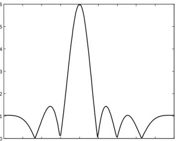
1. Introduction 3 0 20 40 60 80 100 120 140 160 180 0 1 2 3 4 5 6 Directi on (deg) B eam pat tern

Figure 1.1: Beam pattern associated with an azimuth direction 80 using a 6-antenna ULA

beamformer is chosen properly, the power pattern of the resolved signal will exhibit a maximum at the direction of the impinging signal. This principle is named conventional beamforming [3], [4]. In wireless communications, beam-forming is an e¤ective approach used to improve link quality with respect to a particular direction, in the presence of interfering signals.

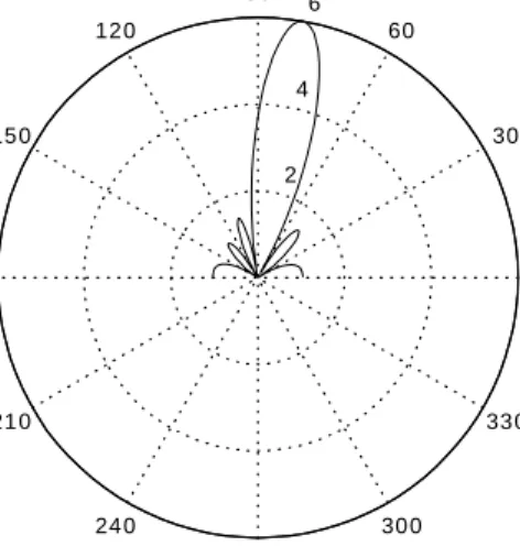
The number of elements and inter-element spacing jointly specify a spatial aperture for array data collection. In most of the cases, the distance between adjacent two elements is set to equal and in half wavelength, due to a scaling factor in the model of the array response vector which is also known as array manifold vector or steering vector. The more elements the higher gain can be provided by the array and the narrower the beamwidth, where the latter indicates the improvement of the spatial discrimination capability. An illus-trative example of the power gain (beam pattern) provided by a conventional beamformer is shown by Fig. 1.1, and its polar plot (a beam) is provided by Fig. 1.2.

2 4 6 30 210 60 240 90 270 120 300 150 330 180 0 Directi on (deg)

Figure 1.2: A polar plot for beam pattern associated with an azimuth direction 80 using a6-antenna ULA

In wireless cellular communications, an important application of beamform-ing is to minimize the co-channel interference (CCI) which arises from cellular frequency reuse. If the desired signal and the interfering signals occupy the same temporal frequency, then temporal …ltering can not be used to separate the desired signal from interference without extra signature is used. However, as the desired signal and interference are less likely to receive from the same direction due to di¤erent locations of the emitters. This directional informa-tion can be exploited for the desired signal using beamforming. An example is the downlink transmit beamforming at the base station that each user’s signal is supported by a di¤erent beamformer for simultaneously transmission.

In particular, at the base station, transmit beamforming o¤ers an attrac-tive performance enhancement over CCI by shaping the radiation pattern of beamformers . This is usually done under an adaptive principle that the beam-formers are derived according to a criterion under certain constraints. An im-portant consideration in using conventional transmit beamforming is that the

1. Introduction 5 Ts Ts Sampling .. . Rx Array Ts x(t) N x1 x[n] ∑ wN w2 w1 N x1 y[n] .. . w the beamformer,

updated according to a criterion

Figure 1.3: A narrowband beamformer as a linear combination of the antenna outputs

supported number of users is limited by the number of antenna elements. For instance, anN-antenna array transmitter is able to simultaneously supportN

users as mathematically N 1 orthonormal vectors (nulls) can be found for

N 1 directions, based on an N-dimensional weight vector. Extra degrees of freedom is available when, e.g., orthogonal codes are employed for each user.

Time-only processing corresponds to a tapped-delay line (TDL) that uses a weighted sum of signal samples and space-only processing corresponds to a narrowband beamformer that uses a weighted sum of antenna outputs. A typical space-only (conventional) receive beamformer w _{2 C}N 1 is illustrated by Fig. 1.3 y[n] = N X k=1 w_kxk[n] =wHx[n] (1.1)

where N is the number of antennas, xk[n] is the nth sample signal at the kth antenna, wk is the associated weight coe¢ cient and y[n] is the beamformer

output.

Associated with the impinging signal is the complex array response vector (also known as array manifold vector) S _{2 C}N 1, representing the complex array response to a unit amplitude plane wave impinging from direction( ; ), compactly written as

S( ; )= exp4 j2 Fc

c r[cos cos ; sin cos ; sin ] T

(1.2)

whereFc is the carrier frequency,cis the speed of light,r2 RN 3 denotes the

geometry of the array elements in the three dimensional space

r= r_x; r_y; r_z (1.3)

and the azimuth and elevation angles are de…ned in the direction-bearing vector [cos cos ; sin cos ; sin ]T. Without loss of generality, plane wave is considered throughout this thesis, thus = 0 . The beam pattern shown by Fig. 1.1 with respect to an azimuth direction ₂[0 ;180 ) can be expressed as

g( ) =_jw( des)HS( )j (1.4)

In addition, if the carrier frequency Fc is considered as an unknown para-meter of interest, then the sensor interval can not be set to in half wavelength because frequency is unknown. It is suggested to set in half wavelength of the intermediate frequency (IF) [6]. A good approach for joint direction-frequency estimation is presented in [6] based on estimation of signal parameters via ro-tational invariance techniques (ESPRIT) [7]. In this thesis, it is assumed that carrier frequency is known constant.

1. Introduction 7 Ts . . . Ts Ts . . . Ts Ts Sampling . . . Rx Array ∑ . . . Ts . . . Ts Ts ∑ . . . ∑ y [ n ] x ( t ) N x 1 w11 w12 w1L w1(L -1 ) wN2 wN 1 wN( L -1 ) wNL Temporal pr ocessing /

equaliser for the

1 st antenna Temporal pr ocessing / Equaliser for the N th antenna F ig u re 1 .4 : A b ro a d b a n d b ea m fo rm er a s te m p o ra ll y w ei g h te d su m a t ea ch re ce iv e a n te n n a

1.2.2

Spatio-Temporal Processing

As discussed in the previous section, an important application of the antenna array is to separate co-channel interfered signals. However, a signal propa-gating through the wireless channel usually arrives at the receivers along a number of di¤erent paths, i.e., multipaths. These paths arise from di¤raction, re‡ection, refraction or scattering of the radiated energy away from the ob-jects. Due to fading (construction and destruction of multipaths plus energy loss), path delay and multiple access, the received signal is degraded and with inter-symbol interference (ISI). To equalise ISI, temporal processing is required to align the delayed signals arriving along di¤erent directions. Hence, a com-bined space-time structure is preferred for combating CCI and ISI, which are the main challenges in wireless communications for higher channel capacity. Papers for spatial and space-time beamforming can be found in [2], [8]-[12].

A typical spatio-temporal (ST) array receiver is depicted in Fig. 1.4. Com-pared to Fig. 1.3 of only spatial …ltering, it is observed that each antenna has been equipped with an L-tap TDL, where a di¤erent weight coe¢ cient is applied for each tap. The output y[n] is the sum of the temporally weighted sum from each equaliser. This space-time structure is also known as a broad-band beamformer from the perspective of signal processing, in contrast to a narrowband beamformer in Fig. 1.3. Signal spread over a broader frequency band corresponds to smaller time processing interval. If the sampling interval

Ts (shown in Fig. 1.4) is a fraction of the symbol period, then the weight

coe¢ cients can be adjusted and thus to shape the frequency response. The outputy[n]of the ST beamformer w_{2 C}N L 1 is given by

y[n] = N X k=1 L X l=1 w_klxk[n l] =wHx[n] (1.5)

1. Introduction 9 as w= [w11; : : : ; w1L; w21; : : : ; w2L; wN1; : : : ; wN L]T (1.6) x[n] = [x1[n 1]; : : : ; x1[n L]; x2[n 1]; : : : ; x2[n L]; xN[n 1]; : : : ; xN[n L]] T (1.7)

Note that it is convenient to treat the spatial beamformer and the ST beam-former in the vector form, thus they can be uni…ed in the same framework.

1.3

MIMO Communication Systems

This section presents the two types of gain that can be provided by using an antenna array, i.e., the diversity gain by beamforming and the multiplexing gain (degree of freedom) by spatial multiplexing.

1.3.1

Diversity Gain

Multiple antennas are an important approach to improve the performance of wireless communication systems. In a multiple-input multiple-output (MIMO) system with multiple transmit and receive antennas, the spectrum e¢ ciency is much higher than the single-antenna system [13]. Based on two di¤erent objec-tives, the MIMO system can either achieve a diversity gain or a multiplexing gain. From the perspective of information theory, two concepts can be uni…ed and a tradeo¤ [14], [15] exists between them.

The philosophy behind diversity is that multiple antennas are used to en-hance the signal-to-noise ratio (SNR). Many successful applications using this principle can be found in, e.g., radar, sonar, acoustics, downlink transmission and medical imaging. In an arrayed MIMO system, the data symbol is trans-mitted by antennas with a beamformer shaping the power radiation towards a direction, and the receive beamformer follows the same principle. Using this

approach, the spatial gain of arrays at two communication sides is focused on a particular path, thus to combat channel fading. This spatial gain is the diversity gain because multiple antennas are utilized to diversify the transmit-ted data symbol through a fading channel. Assume in a system with N(Tx)

transmit and N(Rx) receive antennas, the maximum diversity gain that can be provided isN(Rx)_N(Tx)_{. In the conventional array systems, the main objective}

is to design beamforming vectors in order to increase the diversity gain. It is convenient to use mathematical models to describe this principle. The received signal vector x(t) _{2 C}N(Rx) 1 of a transmitter-receiver antenna array system is given by

x(t) =_Hw(Tx)m(t) + n (t) (1.8)

with a single-path (for illustrative purpose) channel matrix _{H 2 C}N(Rx) _N(Tx)

de…ned by a Rayleigh fading coe¢ cient , a transmit S(Tx) _{2 C}N(Tx) 1 and a receive array manifold S(Rx) _{2 C}N(Rx) ₁

H= S(Rx)S(Tx)H (1.9)

Note that the channel matrix in Eq. (1.9) is modelled as a function of the manifold vectors. However, _H can also be written as

H= 2 6 6 6 6 6 6 4 11 12 1N(Tx) 21 22 2N(Tx) .. . ... . .. ... N(Rx)_{1 N}(Rx)_{2 N}(Rx)_N(Tx) 3 7 7 7 7 7 7 5 (1.10)

where _pq; p = 1; : : : ; N(Rx)_{; q = 1; : : : ; N}(Tx) _{represents the link coe¢ cient}

from the qth transmit antenna to the pth receive antenna with

pq = h S(Rx)i p h S(Tx)Hi q (1.11)

In Eq. (1.8),m(t)is the message signal formed by a sequence of 1sand n (t) is the additive white Gaussian noise (AWGN) vector of independent and

iden-1. Introduction 11 tically distributed (i.i.d.) complex random variables with zero mean and a co-variance matrix_CN(0_N(Rx); 2_nI_N(Rx)). Note thatCN ( )denotes a complex

nor-mal distribution. After multiplied by the receive beamformerw(Rx) _{2 C}N(Rx) 1, the signal estimate is

y(t) = w(Rx)H_Hw(Tx)m(t) +w(Rx)Hn (t) (1.12) The beamformers are designed to provide maximum diversity gain when the beamformers are associated to the path directions, i.e.,

w(Tx) = S(Tx) (1.13) w(Rx) = S(Rx) (1.14) thus y(t) = S(Rx)HS(Rx) | {z } N(Rx) S(Tx)HS(Tx) | {z } N(Tx) m(t) +w(Rx)Hn (t) (1.15) and E jy(t)_j2 = _{j j}N(Rx)N(Tx) 2 (1.16)

where notice that the receive beamformer is orthogonal to noise vector, then it is ready to see the diversity gain Nd=N(Rx)N(Tx) in the above equation.

1.3.2

Multiplexing Gain

During the past decade, driven by the demand of higher channel capacity, multiple antennas have been considered as a means to increase the capacity of a MIMO channel. Raised from a di¤erent point of view, it is suggested that in a MIMO channel, fading can be bene…cial by increasing the degree of freedom available from the channel [16]-[18]. If the fading coe¢ cient for each transmit-receive antenna link is i.i.d. random variables, then the channel matrix is highly possible well-conditioned, ideally of full column-rank. This indicates a maximum of Nm = min N(Tx); N(Rx) independent parallel spatial channels

can be utilized to support multiple information streams. This principle is named spatial multiplexing, the gain of which depends on Nm. As opposed to

transmit scalar data symbol in the diversity scheme, independent data streams are transmitted to increase channel capacity. Correspondingly, a pre-coding and a post-coding matrix are required for channel diagonalization.

In a multiplexing MIMO system, coding matrices are required to support the degree of freedom o¤ered by the fading channel. The received signal vector is given by

x(t) = _HW(Tx)m(t) + n (t) (1.17)

wherem(t)_{2 C}N(Tx) 1_{is the signal vector of normally distributed i.i.d. random}

variables with _N(0;1) and Nm is the number of independent data streams

(i.e., multiplexing gain), _W(Tx)

2 CN(Tx) N(Tx) _{is the pre-coding matrix, and}

the entries of_Hare complex Gaussian random variables. After multiplied by a post-coding matrix _W(Rx)

2 CN(Rx) N(Rx)_{, the vector estimate y(t)}

2 CN(Rx) 1

is obtained

y(t) =_W(Rx)H_HW(Tx)m(t) +_W(Rx)Hn (t) (1.18) The coding matrices can be designed using the singular value decomposition (SVD) of the channel matrix, such that

H = _UDV (1.19)

W(Tx) = _V (1.20)

W(Rx) = _U (1.21)

where _U and _V are respectively an N(Rx) _N(Rx) _{and an N}(Tx) _N(Tx)

uni-tary matrix, and _D is an N(Rx) _N(Tx) _{rectangular matrix with non-negative}

real numbers on the diagonal and zeros on the o¤-diagonal. The diagonal ele-ments _fd1 d2 : : : dNmg are ordered singular values of H. Then a linear

1. Introduction 13 transformation is given by y(t) = _{U| {z }}H_U IN(Rx) DV_{| {z }}HV IN(Tx) m(t) +_W(Rx)Hn (t) = _Dm(t) +_W(Rx)Hn (t) (1.22) and furthermore E jjy(t)_jj2 = Nm X i=1 d2_i (1.23)

whered2_i,i= 1; : : : ; Nm, are eigenvalues ofH. It is observed in Eq. (1.23) that

the energyd2

i provided by the channel is utilized by the multiplexing approach

to increase the energy of received signal, thus the more paths the better. Comparing Eq. (1.16) and Eq. (1.23), it is seen that the diversity gain

Nd contributes in the form of multiplication while the multiplexing gain

con-tributes as the number of the addition terms. Proof and explanation of diversity-multiplexing gain tradeo¤ can be found in [15].

1.4

Spectrum Sharing Systems

This section introduces the emergence of cognitive radio, its development in the past decade and motivations for the proposed model in Chapter 4. Re-cently, many solutions have been proposed for the prototypes of cognitive radio. However, those prototypes have been classi…ed into underlay, overlay and interweave paradigms from the information theory perspective [19], where these paradigms will be introduced in the next section. The emphasis in this thesis is on integration of MIMO technology into underlay cognitive radio, i.e., MIMO cognitive radio.

1.4.1

Background of Cognitive Radio

As the steadily increasing demand for new wireless services and applications, as well as the increasing number of wireless users, the available spectrum suited for commercial wireless utilization are overpopulated. Since radio spectrum is a natural resource, communications in the same frequency and region at the same time cause interference to coexisting wireless users. Therefore advanced technologies and new spectrum allocation policies are required for the evolution of wireless communications and this is the intrinsic cause to the emergence of cognitive radio [20].

The current spectrum allocation policy does not evolve with the consumer-driven evolution of new wireless technologies, devices and services. The current spectrum policy divides radio spectrum into distinct frequency bands for spe-ci…c uses. Licenses for these blocks are assigned to groups and companies. The main advantage of this approach is that a spectral block is exclusively controlled by a licensee so the interference between its users can be unilater-ally managed. An obvious bene…t is the guaranteed quality of service (QoS). The main disadvantage of this approach is that the block allocation and exclu-sive assignment potentially limit more e¢ cient utilization of spectrum when the number of users is increasing. Driven by the demand for extra spectrum, careful and extensive measurements directed by the Federal Communication Committee (FCC) [21] and Ofcom (UK communications regulator) [22] have revealed that spectrum under-utilization is actually a spectrum access prob-lem rather than lack of natural resources. The e¢ ciency of frequency air tra¢ c highly depends on time, location, technology and policy. Thus the current li-censed and unlili-censed paradigms are not essential barriers of accommodating more wireless devices if these devices can exploit advanced technology to con-trol their interference caused to the coexisting devices under an acceptable threshold. Generally, there are various types of solutions. Cognitive radio,

1. Introduction 15 standing for broad connotations, arises from the idea that enables cognitive communication to coexist with licensed devices while keeping the minimal im-pact on the licensed users. It is possible that cognitive radio will evolve in the future to a wireless network with arti…cial intelligence, but its research at present is based on the advances in wireless communication technologies.

More speci…cally, the term cognitive radio was …rst coined by Mitola [23], [24] in 1999. Built on a software-de…ned radio (SDR) platform, cognitive radio is promoted as a context-aware radio [25]. Its intelligence relies on:

Automatically sensing radio environment and making correct decisions;

Recon…guring transmission strategies including protocols, coding and digital signal processing methods in order to adapt to the opportuni-ties.

The idea of SDR-based cognitive radio is certainly an application of the concept: dynamic spectrum access [26]. Dynamic spectrum access aims to improve spectrum e¢ ciency through dynamic spectrum allocation or oppor-tunistic spectrum access, where both have to detect the spectrum opportunities in the sense of space and time. In order to …nd the opportunities, spectrum sensing plays a particular important role. The main challenges involves de-tection of space-time spectrum holes [20], identi…cation of existing users and the shadowing problem [27]. Spectrum sensing can be reduced to a classic signal processing problem as discussed in [27], in which the advantages and disadvantages of matched …lter, energy detector and cyclostationary feature detector are discussed respectively. Furthermore, in some situation when the licensed user’s signal is blocked or strongly interfered, the received primary signal could be too weak to be detected, which causes a high probability of misdetection. This is known as the shadowing problem. To overcome shad-owing, distributed sensing is presented in [28]-[30]. In addition, compressed

sensing and a wavelet approach are respectively employed by [31] and [32] for wideband spectrum sensing.

Dynamic spectrum access has attracted a lot of attention and much contri-bution has been made to spectrum sensing. Its importance to cognitive radio lies in the ‡exibility introduced into the current static spectrum management policy. However, dynamic spectrum access is not the only solution to cogni-tive radio. Since the introduction of cognicogni-tive radio [25], the initial ideas have been further developed to a variety of di¤erent versions. Behind the various interpretations of cognitive radio lies a common feature: awareness of its en-vironment [20], [19]. From the perspective of information theory, awareness of its environment can be interpreted as utilization of network side information [19], which involves:

Channel status;

Codebooks or messages used by other nodes and;

User activity.

According to the types of the available network side information, cogni-tive radio systems can be classi…ed into: underlay, overlay and interweave paradigm [26], [19], which are shown by Fig. 1.5.

In the underlay paradigm, users are known as primary (licensed) users and secondary (cognitive) users. This paradigm is based on the assumption that secondary user has knowledge of the interference caused by its transmitter to the primary receiver (PRx). Therefore, the secondary user can constrain the interference below an acceptable threshold. In another word, the secondary user requires some knowledge of the channel state information (CSI) to satisfy this condition. Technologies, such as beamforming [2], [8], spread spectrum and ultrawideband (UWB) communications, are candidates to meet the

re-1. Introduction 17 Licensed radio & cognitive radio (CR )

Spectrum Sharing Network

Underlay Paradigm

Overlay Paradigm

Interweave Paradigm

Beamforming techniques

Coding techniques

Dynamic spectrum access

techniques

CSI availabl

e at CR Tx

Message side information

available at CR Tx CSI by spectrum s ensing F ig u re 1 .5 : P ro to ty p es o f co g n it iv e ra d io

quirement. Particularly, with the employment of an antenna array at the sec-ondary transmitter (STx), the main radiated power can be steered away from the direction of the PRx so as to constrain the interference. Alternatively, the signal can be spread under the noise ‡oor and despread at the secondary receiver (SRx).

The most important assumption in the overlay paradigm is that cognitive radio has the knowledge of existing users’codebooks and transmitted signals. Like the underlay paradigm, overlay paradigm enables simultaneous transmis-sion as well. Knowledge of a existing user’s codebook even its messages (if possible) can be exploited at cognitive transmitter to mitigate interference seen at the existing users and other cognitive users. As an alternative, this knowledge can also be used at the cognitive receiver for completed interference cancellation. This idea needs sophisticated coding technique, for instance, dirty paper coding (DPC) [33].

Apart from using the CSI in the underlay paradigm and the message side information in the overlay paradigm, the interweave paradigm allows cognitive systems to exploit the activity side information of the existing user. The cognitive system periodically monitors the spectrum and detects opportunities for the cognitive users to communicate with the minimal impact to the active users. This is exactly the concept of dynamic spectrum access as discussed previously.

1.4.2

MIMO Cognitive Radio

In this thesis, it is concerned with underlay paradigm using antenna arrays. The objective is to maximize the sum capacity1 of the spectrum sharing sys-tems using transmit beamforming matrix.

1_{The capacity-achieving strategy is dirty paper coding [33] which is a nonlinear coding} method. Here, the maximal capacity is referred to that the linear transformation can achieve.

1. Introduction 19 Conventional beamforming is not a capacity-achieving strategy in high SNR region for a MIMO channel with large number of multipaths (not clustered) [13]. For a transmit weight vector, its transmit covariance matrix is of rank-one. It implies that only one e¤ective data stream can be supported at the transmitter, thus the degree of freedom (usually more than one) provided by multipath channel is not fully used. This leads us to think of transmitting multiple data stream at the transmitter. In order to make this idea possible, it is proposed to use a full column-rank beamforming matrix (or pre-coding matrix) instead of a beamforming vector. The relationship between these two weighting strategies is the tradeo¤ between diversity and spatial multiplexing, which is revealed in [14].

The rank of the beamforming matrix is decided by the minimal number of antennas of the transmit and receive antenna arrays, usually referred to as the degree of spatial multiplexing. Increasing the rank of transmit covariance ma-trix indicates that more eigen channels can be supported and correspondingly a higher capacity will be achieved. In the traditional beamforming, beams are pointing to the DODs of multipaths in a channel, but in the eigen beamform-ing the e¤ective beams are pointbeamform-ing towards the directions of the eigenvectors of the e¤ective channel. In addition CSI is required at the transmitter.

Since more independent parallel eigen channels can be supported by the beamforming matrix, the capacity is thus higher than that at most one eigen channel is supported by a beamforming vector. If the transmitter is able to provide high transmitted power, i.e., high SNR (assume noise power is constant), then this power can be used under water-…lling [34] principle to further improve the channel capacity.

MIMO cognitive radio [1], [35], [36], [37] has attracted a lot of attention. A typical decentralized setup is presented in [35], exclusively focused on im-proving the performance of cognitive radio network. It assumes in [35] that

multiple non-cooperative MIMO cognitive transmitter-receiver pairs compete for the spectrum resource that is available from the licensed users. The equi-librium of competition eventually falls into the well-known concept of Nash equilibrium (NE) in game theory (e.g., game theory for communications in [38], and [39]). The sum capacity of cognitive links is considered as the util-ity function and it is optimized using an iterative water-…lling algorithm (for classic water-…lling algorithm see [34]), which was …rst introduced in [40], [41]. In addition, in [35] constraints are set to limit the transmitted power for each cognitive transmitter. Focused as well on the cognitive radio network, [42] optimizes the capacity of a single cognitive link under the constraints of the transmitted power and interference caused to the non-cognitive receivers. The solution also depends on an iterative water-…lling algorithm. Furthermore, centralized setup for cognitive network can be found in [37].

In Chapter 4, a simple spectrum sharing network is formed using a primary and a secondary transmitter-receiver antenna array system. It is proved that an equilibrium can be achieved when both receiver employ a single-user receiving strategy. The sum capacity is optimized using a joint water-…lling algorithm. Some key points di¤erent to [1], [35], [36], [37] are summerised as follows:

Formulated a 2-transmitter vs. 2-receiver spectrum sharing network;

Considered sum capacity of the primary and the secondary network and;

Chapter 2

Direction-of-Departure

Estimation Using Cooperative

Beamforming

A novel approach is presented in this chapter for estimating DOD in a frequency-selective multipath channel, where both the transmitter and receiver employ an antenna array [43]. In general, estimating direction-of-arrival (DOA) of a path is a well-known and well-investigated problem and it can be implemented by the receiver. While DOD cannot be estimated simply by the receiver due to the unknown propagation characteristics of the channel, e.g., channel re-‡ection and de¤raction. Therefore, the help of the transmitter is necessary. Brie‡y, the cooperation between the transmitter and receiver is the key to DOD estimation, which will be shown in this chapter.

In particular, the proposed approach in this chapter exploits the cooper-ation between the transmit and receive beamformers, such that the transmit beamformer rotates its mainlobe in a synchronized manner that is known to the receiver. This operation allows DODs of the multiple paths to be estimated at the receiver by making a set of power measurements. The performance of

the proposed approach is investigated using computer simulations and further studies on channel capacity with respect to DODs is presented.

2.1

Signal Model

It is well-known that the employment of antenna arrays [8] can signi…cantly improve the diversity gain of a communication system. In the antenna array systems, DOD is an important parameter for the transmit beamformer which steers the radiating power towards a particular direction in order to improve the link quality and mitigate interference. The maximum gain occurs when the transmission is aligned along with the direction of the channel [44], i.e., DOD of the channel. To be able to form a beam to steer the signal, the transmitter needs to know the DOD. Motivated by this fundamental view, a simple and e¤ective approach for estimating DOD is proposed in this chapter.

A typical scenario is illustrated using two re‡ected paths in Fig. 2.1, where DODs (Tx)1 and

(Tx)

2 are to be estimated given the DOAs (Rx)

1 and

(Rx)

2 .

A number of DOD estimation approaches are presented in [45]-[49]. In [45] a test bed is presented for the DOD estimation. In this system, a signal is transmitted using an omnidirectional monopole antenna and received by a uniform linear array (ULA) at the receiver. The transmit antenna is placed at a number of positions, such that a virtual-cross array can be formed in order to have an arbitrary array shape. In the modelling, the Doppler shift, path delay, DODs and DOAs are built into the impulse response of the channel. By moving the transmitter antennas at a constant speed, the received mea-surements are processed using estimation of signal parameters via rotational invariance techniques (ESPRIT) algorithm [7]. The post-processing consecu-tively removes the Doppler e¤ects, estimates the path delays and DOAs and, …nally the DODs. This double-directional channel model [45] is later on used

2. Direction-of-Departure Estimation Using Cooperative Beamforming 23 in [46] but with a di¤erent strategy that a switched multibeam antenna is employed at the transmitter. The idea of sequential estimation [45] is also employed in [47] for DOD estimation. However, all of the above approaches are limited to linear antenna array geometries.

1 θ(Tx) 2 θ(Tx) 1 θ(Rx) 2 θ(Rx) Tx array Rx array

Figure 2.1: Two multipaths with respective DODs and DOAs, where the re-‡ections are due to unknown positions

In this chapter, a novel approach is proposed based on power estimation at the receiver, which is simple and e¤ective. It exploits the concept that when the mainlobes of the transmit and receive beamformers are respectively steered towards the DOD and DOA of a speci…c path, then the maximum received power will be observed at the receiver. Hence, "rotating" the trans-mit beamformer causes a change of the amplitude of the received power, and consequently a DOD can be identi…ed as a particular direction that provides the maximum power estimate at the receiver. This idea is not limited to the array geometry, receiver type or the presence/absence of the line-of-sight.

Consider a receiver with an array ofN(Rx)_{antennas receiving a signal via a}

K-path frequency-selective channel from a transmit array of N(Tx) antennas, where the vector-input vector-output (VIVO) channel is illustrated by Fig. 2.2.

The received baseband complex signal vectorx(t; )_{2 C}N(Rx) ₁

is given by x(t; ) = K X k=1 p P _kS(Rx)_k S(Tx)_k Hw(Tx)( )m(t k) + n (t) (2.1)

ß

ß

S

S

S

S

_S

ß

S

x

(

t

)

w

n

(

t

)

w

m

(

t

)

∑

m

(

t

)

A

B

C

2. Direction-of-Departure Estimation Using Cooperative Beamforming 25 where _{2 D} denotes the scanning direction at the transmitter and has been added tox(t)as a parameter of interest. The symbol_Drepresents the scanning sector. The noise vectorn (t)_{2 C}N(Rx) 1 is assumed to be complex AWGN hav-ing zero mean and a covariance matrix, i.e., N(0; 2

nIN(Rx)). The transmitted

baseband signal m(t) is randomly generated with unit power and m(t k)

is its delayed version with k the delay of the kth path. The complex

fad-ing coe¢ cient is denoted by k for the kth path and P is the transmitted

power of the signal. The transmit beamformer, using unity norm weight vector

w(Tx)( ) _{2 C}N(Tx) 1, is formed towards a scanning direction . The transmit array manifold vectorS(Tx)_{k 2 C}N(Tx) ₁

, for azimuth DOD (Tx)_k of thekth path, is given by

S(Tx)_k ,S (Tx)_k = exp j2 Fc

c r

(Tx)_u(Tx)

k (2.2)

where Fc is the carrier frequency, c is the speed of light, r(Tx) 2 RN

(Tx) ₃

denotes the geometry of the transmitter array elements and

u(Tx)_k =hcos (Tx)_k ;sin (Tx)_k ;0iT (2.3) is the transmitter wave-number vector. Similarly,S(Rx)_k ,S (Rx)_{k 2 C}N(Rx) ₁

is the receiver array manifold for DOA (Rx)_k . Without loss of generality, the elevation angle is assumed equal to zero throughout this chapter.

2.2

Proposed Cooperative Beamforming

It is assumed that the number of DOAs can be detected by the information theoretic criteria [50], which is an order detection problem in array processing [51]. These are based on two classic algorithms for model selection:

1. Akaike information criterion (AIC) by Akaike [52];

2. The minimum description length (MDL) by Rissanen and Schwartz [53], [54], [55].

Performance analysis on the information theoretic criteria (AIC and MDL) are presented in [56]-[59] and the robustness of MDL is investigated in [60]. A novel approach using the transformed Gerschgorin Radii is introduced in [61]. This detector, as well as the MDL, is consistent and it provides improved detection performance over small data samples or coloured Gaussian noise. Source number estimation is a well-known and well-investigated problem, so either the number of DOAs or the impinging signals at the receive antenna array is assumed known throughout this thesis.

With reference to Fig. 2.3-2.6, the proposed cooperative beamforming can be described in four steps. As shown in the …gures, a representative example of a 2-path channel is used. A feedback link from receiver to transmitter and a perfect synchronization between the transmitter and receiver are assumed.

DOA estimation

algorithm

θ

x (t,θ)

Rotate beam with a known velocity 1 θ(Tx) 2 θ(Tx) 1 θ(Rx) 2 θ(Rx) Tx array Rx array 1 θ(Rx) 2 θ(Rx)

(

)

Figure 2.3: The1st step of the proposed approach: rotate the Tx beamformer and estimate DOAs at the Rx

Step-1 (Fig. 2.3): Firstly, the DOAs of all the paths are estimated. The

mainlobe of the transmitter rotates with a certain …xed angular velocity over a set of scanning directions, e.g., =_f1 ;2 ; : : : ;180 _g. For a particular direc-tion , a transmit beamformer w(Tx)_{( ) is constructed using the transmitter}

manifold vector and it is normalized to have unity norm

w(Tx)( ) = S

(Tx)_{( )}

2. Direction-of-Departure Estimation Using Cooperative Beamforming 27 With the transmit beamformer steering to di¤erent directions, the receiver receives a number of signal samples with respect to each direction (note that synchronization is assumed between the transmitter and receiver). The DOAs and path delays of K paths can then be estimated based on these received signal using, for instance, super-resolution algorithm for DOA estimation (e.g., the MUltiple SIgnal Classi…cation, MUSIC, algorithm [62]). Note that delay estimation algorithms are not considered in this proposed approach.

Step-2 (Fig. 2.4): The receiver steers one mainlobe to each estimated

DOA by constructing beamformers w(Rx)_{k 2 C}N(Rx) 1, k = 1; : : : ; K. There are a number of choices available, e.g., the Wiener-Hopf (WH), MMSE or subspace-type beamformers. Two typical receive beamformers are presented in the next section.

Form beamformer per estimated DOA 1 θ(Tx) 2 θ(Tx) 1 θ(Rx) 2 θ(Rx) Tx array Rx array x (t,θ)

Figure 2.4: The2nd step of the proposed approach: steer the mainlobes of the Rx towards the estimated DOAs

Step-3 (Fig. 2.5): With a receive beamformer steered to a particular DOA,

for every transmit scanning direction ,L snapshots ofx(t; )are collected at the receiver. Note that the velocity of rotations at the transmitter is known to the receiver. Then the powerPk( ) at the output of the receive beamformer is estimated for the kth path, given as follows

Pk( ) = 1 L L X l=1 jw(Rx)_k Hx(tl; )j2 , 8 k; (2.5)

wherew(Rx)_k is the receive beamformers constructed inStep-2 and the subscript

direction that yields the maximum power estimate Eq. (2.5), such that (Tx) k = arg maxPk( ), 8 k; (2.6) Collect data per DOA Power estimation for DODs 2 1 x (t,θ) θ

Rotate beam with a known velocity 1 θ(Tx) 2 θ(Tx) 1 θ(Rx) 2 θ(Rx) Tx array Rx array 1 θ(Tx) 2 θ(Tx)

(

)

Figure 2.5: The3rd step of the proposed approach: rotate the Tx beamformer and estimate the received power for each rotation, then estimate DODs as the directions associated with the largest powers

Step-4 (Fig. 2.6): The DOD estimates are fed back to the transmitter using

a feedback link. With the transmit and receive beamformers steered to DODs and DOAs respectively, the identi…ed paths are utilized by a number of beams. Furthermore the maximum ratio combining (MRC) approach can be used to combine the paths, therefore the overall link quality is improved. Finally, the implementation procedure of the proposed approach is summarized in Table 2.1. Feedback channel 1 θ(Tx) 2 θ(Tx) 1 θ(Rx) 2 θ(Rx) Tx array Rx array

Figure 2.6: The …nal step of the proposed approach: feed back the estimates to Tx and steer the mainlobes of Tx towards these DODs

2. Direction-of-Departure Estimation Using Cooperative Beamforming 29

Table 2.1: Implementation procedure of the cooperative beamforming

DOA Estimation :

1a. rotate w(Tx)_{( ) using Eq. (2.4),}

8 ;

1b. estimate (Rx)_k ,₈ k;

DOD Estimation :

2. steer w(Rx)_k using Eq. (2.7) or Eq. (2.8),₈ k; 3a. rotate w(Tx)( ) using Eq. (2.4), ₈ ;

3b. calculatePk( ) at receiver with Eq. (2.5), 8 k, ;

3c. identify (Tx)_k using Eq. (2.6),₈ k;

Feedback :

4. feed the estimated DODs to transmitter and steer the transmit

mainlobes (one per DOD)

2.3

Receive Beamformer

Two typical receive beamformers are considered for comparison, respectively based on the WH [63] and the subspace [63] method. The WH method max-imizes the output SNR [63] while the subspace beamformer are maximizing the output signal-to-interference ratio (SIR) [64]. The subspace method here considers the signals received via other multipaths as unwanted interference and an asymptotic cancellation is provided. Other criteria subject to minimum variance distortionless response (MVDR) and minimum bit error rate (BER) can be found respectively in [63] and [65].

1. The well-known WH beamformer is given by

w(Rx)_k =_Rxx1S(Rx)_k (2.7)

whereS(Rx)_k is the receive array manifold vector for thekth path, formed based on the estimated (Rx)_k , and the covariance matrix of the received signal is given by _Rxx =E

n

x(t; )x(t; )Ho_{2 C}N(Rx) N(Rx).

2. The subspace-type beamformer is based on the projection operator. It isolates (receives) one single path while providing cancellation of the other paths as unwanted interference. This operation provides, asymp-totically, complete self-interference cancellation. This beamformer is de-…ned as

w(Rx)_k =_P?_kS(Rx)_k (2.8)

where S(Rx)_k is the receiver manifold vector of the kth path and _P?_{k 2} CN(Rx) _N(Rx)

is the complement projection operator onto the subspace spanned by the columns of matrix_Sk. That is

P?k =IN(Rx) S_k SH_kS_k

1

SHk (2.9)

where_Sk 2 CN

(Rx) _{(K 1)}

is the matrix with the receiver manifold vectors for all paths except the kth path

Sk =

h

S(Rx)₁ ; : : : ; S(Rx)_{k 1}; S_k(Rx)₊₁; : : : ; S(Rx)_K i, k 2 (2.10)

2.4

Performance of Cooperative Beamforming

2.4.1

Simulation Results

Without any loss of generality, assume that both the transmitter and receiver use uniform linear antenna arrays of half-wavelength spacing with the numbers of elements N(Tx)_{; N}(Rx) _{= (4;8). Assume that the number of multipaths is}

2. Direction-of-Departure Estimation Using Cooperative Beamforming 31

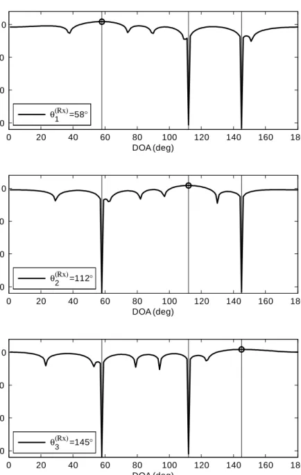
K = 3, where DODs = [38 ;62 ;115 ] and DOAs = [58 ;112 ;145 ]. Channel fading coe¢ cients are complex random variables with an amplitude of _{j kj} = 0:5. The baseband transmitted signal is randomly generated with zero mean and variance _E m(t)2 = 1. The transmitted power is denoted byP and the channel noise is assumed to be 10 dB below P, i.e., SNR = P= 2_n = 10 dB. The transmit beamformer rotates with a …xed angular velocity that allows the collection at the receiver of L = 500 snapshots per scanning direction

=_f1 ;2 ; : : : ;180 _g. The scanning sector is set to_D=_f1 ;2 ; : : : ;180 _g. In Fig. 2.7 and Fig. 2.8, the receive beam pattern of each multipath by respectively the WH and subspace-type method is shown by the sub…gure. Please note that in Fig. 2.7, nulls are not necessarily provided to suppress the self-interference from other paths but the overall aim is to improve SNIR. For instance in Fig. 2.7, DOA (Rx)1 = 58 is nulled by the second and the third

receive beam patterns, but DOA (Rx)₂ = 112 is not nulled by the …rst beam pattern and neither DOA (Rx)3 = 145 is nulled by the …rst beam pattern. The

case is di¤erent in Fig. 2.8 that very deep nulls are provided by the projection operator, and in each sub…gure the unwanted paths are strongly suppressed.

Fig. 2.9 shows the estimated transmit array patterns and DODs for a 3-path channel, where these transmit array patterns are individually estimated and plotted in one …gure. Therefore, even very close DODs = [38 ;40 ;115 ] can be identi…ed as shown by Fig. 2.10. DODs are quickly identi…ed as the directions associated with the three peaks. Both WH and the subspace-type receive beamformer give very similar pattern shapes but di¤erent magnitudes, which can be removed by normalizing the pattern of Fig. 2.11.

The standard deviation (STD) of the estimation error vs. SNR and the number of snapshots L are respectively presented in Fig. 2.12 and Fig. 2.13. In the high SNR region (to the right of SNR = 8 dB) of Fig. 2.12, the STD (in degree) of the subspace-type beamformer is smaller than that of the WH

0 20 40 60 80 100 120 140 160 180 -15 -10 -5 0 5 10 15 20 DOA (deg) Rx beam pat ter n (dB ) θ(Rx) 1 =58° 0 20 40 60 80 100 120 140 160 180 -15 -10 -5 0 5 10 15 20 DOA (deg) Rx beam pat ter n (dB ) θ(Rx) 2 =112° 0 20 40 60 80 100 120 140 160 180 -15 -10 -5 0 5 10 15 20 DOA (deg) Rx beam pat ter n (dB ) θ(Rx) 3 =145°

Figure 2.7: Rx beam patterns using Wiener-Hopf beamformer; K = 3;

D 2 [0 ;180 ]; (N(Tx)_{; N}(Rx)_{) = (4;8);} (Tx) _{= [38 ;62 ;115 ];} (Rx) ₌

2. Direction-of-Departure Estimation Using Cooperative Beamforming 33 0 20 40 60 80 100 120 140 160 180 -150 -100 -50 0 DOA (deg) Rx beam pat ter n (dB ) θ(Rx) 1 =58° 0 20 40 60 80 100 120 140 160 180 -150 -100 -50 0 DOA (deg) Rx beam pat ter n (dB ) θ(Rx) 2 =112° 0 20 40 60 80 100 120 140 160 180 -150 -100 -50 0 DOA (deg) Rx beam pat ter n (dB ) θ(Rx) 3 =145°

Figure 2.8: Rx beam patterns using subspace-type beamformer; K = 3;

D 2 [0 ;180 ]; (N(Tx)_{; N}(Rx)_{) = (4;8);} (Tx) _{= [38 ;62 ;115 ];} (Rx) ₌