A novel feature extraction for anomaly detection of roller bearings based on performance improved Ensemble Empirical Mode Decomposition and Teager-Kaiser energy operator / TABRIZI ZARRINGHABAEI, ALI AKBAR; GARIBALDI, Luigi; FASANA, ALESSANDRO; MARCHESIELLO, STEFANO. - In: INTERNATIONAL JOURNAL OF PROGNOSTICS AND HEALTH MANAGEMENT. - ISSN 2153-2648. - ELETTRONICO. - 6(2015), pp. 1-10.
Original
A novel feature extraction for anomaly detection of roller bearings based on performance improved
Ensemble Empirical Mode Decomposition and Teager-Kaiser energy operator
Publisher: Published DOI: Terms of use: openAccess Publisher copyright
(Article begins on next page)
This article is made available under terms and conditions as specified in the corresponding bibliographic description in the repository
Availability:
This version is available at: 11583/2643228 since: 2020-04-29T11:19:55Z
International Journal of Prognostics and Health Management, ISSN 2153-2648, 2015 026
A Novel feature extraction for anomaly detection of roller bearings
based on performance improved Ensemble Empirical Mode
Decomposition and Teager-Kaiser Energy Operator
Ali Tabrizi1, Luigi Garibaldi2, Alessandro Fasana3 and Stefano Marcchesiello4
1,2,3,4 Dynamics & identification research group, Department of mechanical and Aerospace Engineering, Politecnco di Torino, Corso Duca degli Abruzzi 24, 10129 Torino, Italy
[email protected] [email protected] [email protected] [email protected]
ABSTRACT
Although Ensemble empirical mode decomposition (EEMD) method has been successfully applied to various applications, features extracted using EEMD could not detect anomalies for roller bearings, especially when anomalies includes small defects. In this study a novel feature extraction method is proposed to detect the state of roller bearings. Performance improved EEMD, which is a reliable adaptive method to calculate an appropriate noise amplitude is applied to decompose the acceleration signals into zero-mean components called intrinsic mode functions (IMFs). Then, three dimensional feature vectors are created by applying the Teager-Kaiser energy operator (TKEO) to the first three IMFs. The novel features obtained from the healthy bearing signals are utilized to construct the separating hyperplane using one-class support vector machine (SVM). In order to validate the method proposed, a number of operating conditions (shaft speed and load) are considered to generate the data (vibration signals) by means of an assembled test rig. It is shown that the proposed method can successfully identify the states of the new samples (healthy and faulty). The uncertainty of the model prediction is investigated computing Margin and the number of support vectors. It create less complex (less fraction of support vectors) and more reliable (higher Margin) hyperplane than the EEMD method.
1.INTRODUCTION
Since roller bearings constitute one the most important elements of rotating machines, early fault diagnosis of roller bearings is extremely important, especially for high speed, automatic and precise machines. Thus, many research efforts have been focused on fault diagnosis and detection of roller bearings.
Several signal processing techniques exist to decompose a signal and extract informative features for roller bearings. Randall and Antoni (2011) have broadly treated the background of some powerful diagnostic methods for roller bearings in a very useful tutorial paper. Empirical mode decomposition (EMD) is another recent technique, a so-called self-adaptive data driven technique, for analyzing multi-component nonlinear and non-stationary signals and brake down them into some elementary modes called Intrinsic mode functions (IMFs). (Huang et al., 1998). However, this technique still holds some drawbacks such as mode mixing problem. Ensemble empirical mode decomposition (EEMD) is a more recent developed method aimed to solve mode mixing problem (Wu & Huang, 2009). Although the EEMD has been successfully applied to damage detection of roller bearings (Lei et al., 2013), it is shown that there are still some cases for which it is not able to recognize introduced novelties.
In this study a new feature extraction method is proposed for novelty detection, which is based on performance improved EEMD and Teager-Kaiser energy operator (TKEO). In
traditional EEMD the amplitude of noise added to the original signal is considered as a predefined constant value. Whereas, in performance improved EEMD (PIEEMD) proposed by the authors (Tabrizi et al., 2015A), amplitude of added noise is adaptively computed for each data point explained in section 2.1.
Teager-Kaiser energy operator (TKEO) technique is a non-linear operator able to track the energy and to identify the instantaneous frequencies and instantaneous amplitudes of signals. Teager (1980) proposed TKEO first for modelling nonlinear speech production. Kaiser (1990) applied it to single time varying signals, for simultaneous modulation of amplitude and frequency. As it detects a sudden change of the energy stream without a priori assumption of the data structure, it can be utilized for vibration based condition monitoring (non-stationary signals). Junsheng et al. (2007) applied the TKEO to each IMFs decomposed by the EMD to extract the instantaneous amplitudes and frequencies. Then
_____________________
Ali Tabrizi et al. This is an open-access article distributed under the terms of the Creative Commons Attribution 3.0 United States License, which permits unrestricted use, distribution, and reproduction in any medium, provided the original author and source are credited.
envelope spectra were obtained using the spectrum analysis to look for characteristic frequencies of damaged roller bearings. Li, Fu & Zhang (2009) applied the TKEO to the original vibration signals and characteristic frequencies were extracted from envelope spectra. Li, Zhang & Tang (2009) implemented a novel method to recognize faults of roller bearing based on Teager-Huang transform (THT) introduced by Cexus & Boudraa (2006). In all those studies, it was investigated how to identify a big damage size (1mm in depth, 1.5mm width of the groove). Feng et al. (2011) utilized the Fourier spectrum of Teager energy to identify the characteristic frequency of faulty bearings (very big defect sizes: 2mm diameter and 1mm depth). Liu et al. (2013) presented an approach to bearing fault diagnosis based on the TKEO and the Elman neural network. The wavelet packet was used to reduce noise existing in the Teager energy signal, and then feature vectors were extracted from the Teager spectrum. Rodriguez et al. (2013) transformed the vibration signal to the Teager-Kaiser domain and featured it with statistical and energy-based measures. The diagnosis was performed with the neural network and the least square support vector machine (LS-SVM). Kwak et al. (2014) applied the TKEO in a combination with minimum entropy deconvolution (MED) to detect a defective roller bearing in terms of Kurtosis.
There are various pattern recognition methods such as Artificial neural network (ANN) and Support vector machine (SVM) which was introduced by Vapnik (1995). The SVM is a relatively new computational learning method based on statistical learning theory which has been applied successfully to numerous applications (Widodo & Yang, 2007). It can solve the learning problem with a smaller number of samples. Thus, taking into account the fact that acquiring sufficient faulty samples is not applicable in practice, the SVM has been used in a number of fault diagnosis problems successfully. As in many diagnostic applications, this is the case of a single type of data (the healthy one), one-Class SVM proposed by Scholkopf et al. (2000) can be adopted for anomaly detection.
In this study a new feature extraction method is proposed to detect the state of roller bearings. The signal is decomposed using performance improved EEMD. Then, the three dimensional feature vectors are created by applying TKEO to the first three IMFs of the healthy bearing signals are utilized as input for one-class SVM to construct the separating hyperplane. It is shown that the method proposed can successfully identify the states of the new samples (healthy and anomaly ones). A number of healthy and faulty acceleration signals are analyzed to verify the feature extraction proposed in this study.
The methodology is introduced in two parts, feature extraction in section 2 and pattern recognition in section 3. In feature extraction section, the performance improved EEMD method and Teager-Kaiser energy operator are
introduced in section 2.1 and 2.2, respectively. One-class SVM is introduced as the pattern recognition method used in this study in section 3. The procedure of the novel feature extraction method is explained in section 4. The experimental setup and the data-acquisition process are presented in section 5. The application of the new approach to the acquired data and the results are discussed in section 6. Finally, the paper concludes after some discussion in section 7.
2.FEATURE EXTRACTION METHODS
The In this study informative features introduced, which are extracted by applying Teager-Kaiser energy operator to IMFs obtained using performance improved EEMD. These methods are explained in the next sections.
2.1.Performance improved Ensemble empirical mode decomposition (EEMD)
The EEMD repeatedly decomposes the original signal with added white noise into a series of IMFs by applying the original EMD process, and treats the means of the corresponding IMFs during the repetitive process as the final EEMD decomposition result. The decomposition steps by the EEMD can be summarized as follows:
1. To add a random white noise signal to the acquired original signal:
𝑥𝑗(𝑡) = 𝑥(𝑡) + 𝐴𝑚𝑝 ∙ 𝑛𝑗(𝑡) (1)
where 𝑗 = 1,2, … , 𝑀 and 𝐴𝑚𝑝 is the amplitude of added white noise and M is the pre-determined number of trial.
2. To decompose the obtained signal (𝑥𝑗(𝑡)) into IMFs using
EMD: 𝑥𝑗(𝑡) = ∑ 𝑐𝑖𝑗 𝑁𝑗 𝑖=1 + 𝑟𝑁𝑗 (2) where 𝑐𝑖𝑗 represents the i-th IMF of the j-th trial, 𝑟𝑁𝑗 represents the residue of j-th trial and 𝑁𝑗 is the IMFs number
of the j-th trial.
3. To repeat steps a and b until the predefined ensemble trial number (M) (add different random noise signal each time). 4. To calculate the ensemble means of the corresponding IMFs of the decompositions as the final result (𝑐𝑖):
𝑐𝑖(𝑡) = (∑ 𝑐𝑖𝑗
𝑀
𝑗=1
) 𝑀⁄
(3) where 𝑖 = 1,2, … , 𝐼 and I is the minimum number of IMFs among all the trials.
INTERNATIONAL JOURNAL OF PROGNOSTICS AND HEALTH MANAGEMENT
3
Adding the noise aims to affect the extrema of the original signal so that the intermittency of the components will be removed. Rather than adding a predefined constant amplitude value (such as 0.2 of standard deviation of the signal in the traditional EEMD method), which might not effectively change some extrema, the adaptive method is used to improve the performance of the EEMD (Tabrizi et al., 2015A). After adding a random white noise, by applying the SNR definition (Eq. (4)), the Amplitude value for each data point of a sample is obtained using Eq. (5). Considering an appropriate value for SNR, the extrema of the original signal are influenced adequately.
𝑆𝑁𝑅(𝑡) = 20 log(𝑥(𝑡) (𝐴𝑚𝑝⁄ 𝑗(𝑡) ∙ 𝑛𝑗(𝑡)))
(4)
𝐴𝑚𝑝𝑗(𝑡) = 10−(𝑆𝑁𝑅(𝑡) 20⁄ ) ∙ (𝑥(𝑡) 𝑛⁄ 𝑗(𝑡))
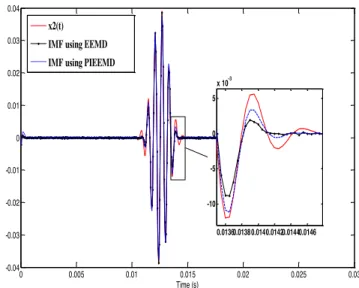
(5) where 𝑗 = 1, … , 𝑀 (𝑗 is the is the ensemble trial number). Tabrizi et al., (2015A) showed that the performance improved EEMD achieves better damage detection results. A simulated signal and its decomposition results using the EEMD and the performance improved EEMD methods are shown in Figures 1 and 2, respectively. Obviously, the IMF obtained using the performance improved EEMD (PIEEMD) is more similar to the high frequency component.
Figure 1. The simulated signal and its high and low frequency components
Figure 2. The high frequency component and the IMF obtained sing the EEMD and the performance improved
EEMD (PIEEMD)
2.2.Teager-Kaiser energy operator (TKEO)
The energy of a signal is the sum of squared absolute value of the signal over a time, which is not the instantaneous summed energy. Kaiser (1990) observed that a second order differential equation is the energy required to generate a simple sinusoidal signal varies with both amplitude and frequency. In order to estimate the instantaneous energy of a signal x(t), Teager-Kaiser Energy Operator (TKEO) is used as an energy tracking operator as follows (Maragos, 1993A):
𝛹[𝑥(𝑡)] = 𝐴2= 𝑥̇2(𝑡) − 𝑥(𝑡) 𝑥̈(𝑡) (6)
where x(t) and x(t) are the first and the second time derivatives of x(t), respectively.
For a discrete time signal x(n) (where n is the discrete time index), using difference to approximate differential, the TKEO can be proposed as:
Ψ[𝑥(𝑛)] = [𝑥(𝑛)]2− 𝑥(𝑛 − 1)𝑥(𝑛 + 1) (7)
As at any instant, only three consecutive samples are needed to estimate the instantaneous TKEO, it is adaptive to the instantaneous changes in signals to resolve transient events. It has some merits such as low computational cost, high resolution of time and frequency and adaptability to instantaneous feature.
The instantaneous frequency and instantaneous amplitude at any time instant of the signal 𝑥(𝑛) are defined as follows (Maragos, 1993B): 0 50 100 150 200 250 300 350 400 450 500 -1 -0.5 0 0.5 1 0 50 100 150 200 250 300 350 400 450 500 -0.04 -0.02 0 0.02 0.04 0 50 100 150 200 250 300 350 400 450 500 -1 -0.5 0 0.5 1 Time (s) x(t) x2(t) x1(t) 0 0.005 0.01 0.015 0.02 0.025 0.03 -0.04 -0.03 -0.02 -0.01 0 0.01 0.02 0.03 0.04 Time (s) x2(t)
IMF using EEMD IMF using PIEEMD
0.01360.01380.0140.01420.01440.0146 -10 -5 0 5 x 10⁻³
𝑓(𝑛) = 1 2𝜋 √ Ψ[𝑥̇(𝑡)] Ψ[𝑥(𝑡)] (8) |𝑎(𝑛)| = Ψ[𝑥(𝑡)] √Ψ[𝑥(𝑡)] (9) They can be represented as follows:
𝑓(𝑛) =1 2 𝑎𝑟𝑐𝑐𝑜𝑠 (1 − Ψ[𝑥(𝑛 + 1) − 𝑥(𝑛 − 1)] 2Ψ[𝑥(𝑛)] ) (10) |𝑎(𝑛)| = 2Ψ[𝑥(𝑛)] √Ψ[𝑥(𝑛 + 1) − 𝑥(𝑛 − 1)] (11)
3.PATTERN RECOGNITION (ONE-CLASS SUPPORT VECTOR MACHINE)
In order to construct a pattern recognition model for novelty detection, only one class of data (features extracted from healthy bearing signals) is used to create one-class SVM model. It constructs a hyperplane around the data, such that its distance to the origin is maximal among all possible hyperplanes and classifies new samples belong to other possible classes as anomaly (Scholkopf et al., 2000). The Margin is defined as:
𝑀𝑎𝑟𝑔𝑖𝑛 = 𝜌 ‖𝑤‖⁄ (12)
In real problems, an exact line dividing the data is not obtainable and we might have a curved decision boundary. Ignoring few outlier data points will create smooth boundary (using slack variables). To separate the data set from the origin, the following quadratic program must be solved (Scholkopf et al., 2000): min (1 2‖𝒘‖ 2+ 1 𝜐𝑙∑ 𝜉𝑖 𝑙 𝑖=1 − 𝜌) (13) subject to {𝑦𝑖(𝒘 ∙ 𝜙(𝒙𝑖)) ≥ 𝜌 − 𝜉𝑖 𝜉𝑖≥ 0 𝑖 = 1, … , 𝑙
where 𝒘 and 𝜌 are the weight vector and the offset parameterizing the hyperplane. 𝜉𝑖 is the slack variable, 𝜐 is
the regularization parameter and represents an upper bound on the fraction of outliers (training errors) and a lower bound on the fraction of support vectors (SVs) with respect to the number of training samples. It is a variable taking values between 0 and 1 that monitors the effect of outliers (hardness
and softness of the boundary around data). The decision function used to label new samples whether they are healthy or outliers (anomaly) is as follows:
𝑓(𝑥) = 𝑠𝑖𝑔𝑛(〈𝑤. 𝑥𝑖〉 − 𝜌) (14)
The SVM could also be applied in a case of non-linear classification by mapping the data onto a high dimensional feature space, where the linear classification is hence possible. A non-linear vector function such as 𝚽(𝒙) =
(𝜑1(𝒙), … , 𝜑𝑙(𝒙)) is used to map the n-dimensional input
vector x onto l dimensional feature space, so that the decision function becomes as follows:
𝑓(𝑥) = 𝑠𝑖𝑔𝑛(〈𝑤. 𝛷(𝑥𝑖)〉 − 𝜌) (15)
By applying the Kernel function as the inner product of mapping functions, it is not necessary to explicitly evaluate mapping in the feature space.
𝐾(𝑥𝑖, 𝑥𝑗) = (Φ(𝑥𝑖) ∙ Φ(𝑥𝑗)) (16)
Various kernel functions could be used such as: Linear 𝐾(𝑥𝑖, 𝑥𝑗) = (𝑥𝑖∙ 𝑥𝑗) 𝑑
Polynomial 𝐾(𝑥𝑖, 𝑥𝑗) = (𝑥𝑖∙ 𝑥𝑗+ 1) 𝑑
Gaussian radial basis function (RBF)
𝐾(𝑥𝑖, 𝑥𝑗) = 𝑒𝑥𝑝 (−𝛾‖𝑥𝑖− 𝑥𝑗‖
2
) Hyperbolic tangent
𝐾(𝑥𝑖, 𝑥𝑗) = 𝑡𝑎𝑛ℎ(𝑘𝑥𝑖∙ 𝑥𝑗+ 𝑐)
As the kernel function defines the feature space in which the training set is classified, the selection of the appropriate kernel function is very important.
Introducing Lagrange multipliers we obtain the dual problem as: 𝑚𝑖𝑛 1 2 ∑ 𝛼𝑖𝛼𝑗 𝑙 𝑖,𝑗=1 𝑲(𝒙𝑖, 𝒙𝑗) (17) Subject to {0 ≤ 𝛼𝑖≤ 1 𝜐𝑙 ∑𝑁𝑖=1𝛼𝑖= 1
If 𝜐 approaches 0, the upper boundaries on the Lagrange multipliers tend to infinity, so the second inequality constraint in Eq. (17) becomes void. As the penalization of errors becomes infinite, it returns to the corresponding hard margin algorithm.
For the positive, non-zero multipliers (support vectors 𝑥𝑖))
INTERNATIONAL JOURNAL OF PROGNOSTICS AND HEALTH MANAGEMENT 5 𝜌 = 𝑤 ∙ 𝜙(𝑥𝑖) = ∑ 𝛼𝑗 𝑙 𝑗=1 𝐾(𝑥𝑗, 𝑥𝑖) (18) Accordingly the non-linear decision function for labelling new samples is represented as follows (𝑥𝑖 represents the
positive, non-zero multipliers called support vectors):
𝑓(𝑥) = 𝑠𝑖𝑔𝑛 (∑ 𝛼𝑖 𝑙 𝑖=1 𝐾(𝑥𝑖, 𝑥) − 𝜌) (19) 4.METHODOLOGY
The goal of this study is to evaluate performance of the proposed feature extraction algorithm in condition detection of a roller bearing.
The fault diagnosis method for the traditional EEMD technique is given as the following (Tabrizi et al., 2014): 1. To collect the acceleration signals of the healthy and defective bearings at three different external loads and two shaft speeds.
2. To apply the EEMD method to decompose the vibration signals into some IMFs. The first m IMFs including the most dominant fault information are chosen to extract the feature. 3. To calculate the total energyEiof the first m IMFs:
𝐸𝑖= ∫ |𝑐𝑖(𝑡)|2 𝑑𝑡
+∞
−∞
(20) 4. To create a feature vector with the energies of the m selected IMFs:
𝐹𝑉 = [𝐸1, 𝐸2, … , 𝐸𝑚] (21)
5. To normalize the feature function:
𝐹𝑉𝑛= [𝐸1⁄ , 𝐸𝐸 2⁄ , … , 𝐸𝐸 𝑚⁄ ]𝐸 (22)
where 𝐸 = (∑𝑚𝑖=1|𝐸𝑖|2)1/2 .
Whereas the proposed feature extraction is implemented as the following steps:
1. To decompose the signal using the performance improved EEMD (PIEEMD) with SNR=10 dB (Tabrizi et al., 2015A) 2. To apply the TKEO to the first m IMFs of each signal. 3. To calculate the sum of each TKEO.
𝑇𝐾𝐸𝑂𝑖= ∑ 𝜓(𝐼𝑀𝐹𝑖)
𝑚
𝑖=1
(23) 4. To create a feature vector with the sum of the calculated TKEO:
𝑇𝐾𝐸 = [𝑇𝐾𝐸𝑂1, 𝑇𝐾𝐸𝑂2, … , 𝑇𝐾𝐸𝑂𝑚] (24)
5. To normalize the feature:
𝑇𝐾𝐸𝑛 = [𝑇𝐾𝐸𝑂1/𝑇𝐾𝐸𝑂𝑡𝑜𝑡, 𝑇𝐾𝐸𝑂2/𝑇𝐾𝐸𝑂𝑡𝑜𝑡, … , 𝑇𝐾𝐸𝑂𝑚/
𝑇𝐾𝐸𝑂𝑡𝑜𝑡]
(25) where 𝑇𝐾𝐸𝑂𝑡𝑜𝑡 = (∑𝑚𝑖=1𝑇𝐾𝐸𝑂𝑖) .
Finally, the training procedure of one-class SVM is carried out by utilizing the normalized feature vectors so far obtained. The 80% of healthy samples are used for training and the rest (remaining healthy samples and all faulty data) are taken as the test samples. Once the training procedure is successfully performed, the parameters are hold to test samples to identify the different work conditions and fault patterns. Cross validation is used to optimize the parameters of pattern recognition method.
5.EXPERIMENTS
The bearing data set (acceleration signals) were collected under various operating conditions using the test rig (Figure 3) developed and assembled by the Dynamics & Identification Research Group (DIRG) at the Department of Mechanical and Aerospace Engineering of Politecnico di Torino. The Kistler triaxial accelerometers (model 8763A500) were used to acquire signals at 102.4 kHz sampling frequency for both healthy and defective roller bearings. The small artificial defects severity over one roller was 150 and 450 microns in diameter. Two different shaft speeds (200 and 300 Hz) and three different external radial loads (1.0, 1.4 and 1.8 kN) were considered to acquire the signals in different operating conditions (as a common industrial set up) in laboratory supervised conditions, allowing speed, load and oil temperature monitoring. The original acquired healthy signals were divided into 30 segments (20 segments for defective bearing) including 10000 data points each, to extract required informative feature vectors. Thus, each healthy signal includes 30 segments which create 30 feature vectors (20 feature vectors for defective bearing) as inputs for the one-class SVM. Selecting samples as the training ones includes all the possible random selections to obtain the maximum classification accuracy rate for training.
(a)
(b)
Figure 3. DIRG test rig (a) the damaged roller used in the tests (b)
6.RESULTS AND DISCUSSIONS
An acquired acceleration signal, its three first IMFs (decomposed using EEMD) and the TKEO of those IMFs are shown in Figure 4. Implementing the methodology to the signals, the normalized energy of IMFs (𝐹𝑉𝑛) for the EEMD
method (using only first three elements of the feature vectors (Tabrizi et al., 2014)) and the normalized 𝑇𝐾𝐸𝑛 for the
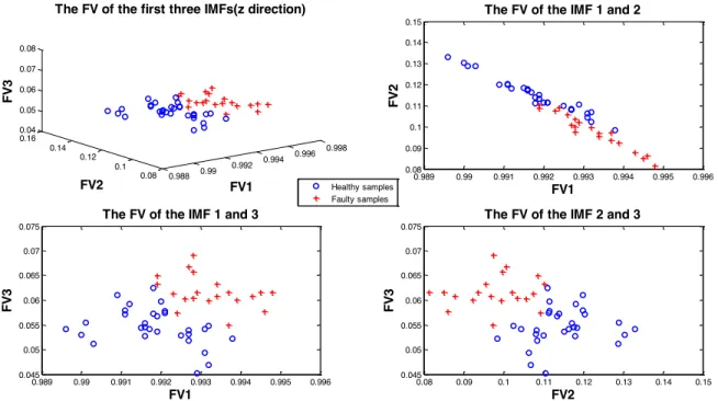
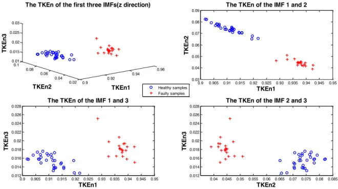
proposed method. 0.3 of standard deviation of each original signal is used as the appropriate amplitude of added noise in the traditional EEMD method (Tabrizi et al., 2015B). As it can be seen in Figure 5, there is a confusion among healthy and faulty samples for the lighter defect size (150 microns) obtained by the EEMD method. In view of this, the novel feature proposed along this study is applied to check whether it can improve the performances of detection. As it can be seen in Figure 6, the healthy and faulty samples are perfectly separable. Thus, it is expected to achieve higher success rate in labelling of new samples.
In Table 1 and Table 2, the results of classification are shown (for shaft speed = 200 and 300 Hz) using one-class SVM. The results are highly dependent on the classification parameters.
The optimal values of the classification parameters ( and ) obtained by cross validation are presented for each methods. The success rates obtained using the proposed feature extraction, are higher so that in some cases there exist considerable differences. For example, with the condition 300 Hz speed and 1.8 kN load, the proposed double steps technique improves the test success rate 23.1%.
(a)
(b)
(c)
Figure 4. A collected acceleration signal (a), first three IMFs (b) and TKEO of the IMFs (c)
0 0.01 0.02 0.03 0.04 0.05 0.06 0.07 0.08 0.09 0.1 -100 0 100 S ig n a l Time (s) 0 0.01 0.02 0.03 0.04 0.05 0.06 0.07 0.08 0.09 0.1 -100 0 100 c1 0 0.01 0.02 0.03 0.04 0.05 0.06 0.07 0.08 0.09 0.1 -50 0 50 c2 0 0.01 0.02 0.03 0.04 0.05 0.06 0.07 0.08 0.09 0.1 -50 0 50 c3 Time (s) 0 0.01 0.02 0.03 0.04 0.05 0.06 0.07 0.08 0.09 0.1 -1 0 1 2x 10 4 T KE O (c 1 ) 0 0.01 0.02 0.03 0.04 0.05 0.06 0.07 0.08 0.09 0.1 -500 0 500 1000 T KE O (c 2 ) 0 0.01 0.02 0.03 0.04 0.05 0.06 0.07 0.08 0.09 0.1 -100 0 100 200 T KE O (c 3 ) Time (s)
INTERNATIONAL JOURNAL OF PROGNOSTICS AND HEALTH MANAGEMENT
7
Figure 5. The normalized energy 𝐹𝑉𝑛 of three first IMFs using EEMD for the 150 microns defect size (Speed = 300 Hz and
load = 1.8 kN)
Figure 6. The normalized 𝑇𝐾𝐸𝑛 of three first IMFs using performance improved EEMD (PIEEMD) for the 150 microns
defect size (Speed = 300 Hz and load = 1.8 kN) 0.988 0.99 0.992 0.994 0.996 0.998 0.08 0.1 0.12 0.14 0.16 0.04 0.05 0.06 0.07 0.08 FV1 The FV of the first three IMFs(z direction)
FV2 FV 3 Healthy samples Faulty samples 0.989 0.99 0.991 0.992 0.993 0.994 0.995 0.996 0.08 0.09 0.1 0.11 0.12 0.13 0.14 0.15
The FV of the IMF 1 and 2
FV1 FV 2 0.989 0.99 0.991 0.992 0.993 0.994 0.995 0.996 0.045 0.05 0.055 0.06 0.065 0.07 0.075
The FV of the IMF 1 and 3
FV1 FV 3 0.08 0.09 0.1 0.11 0.12 0.13 0.14 0.15 0.045 0.05 0.055 0.06 0.065 0.07 0.075
The FV of the IMF 2 and 3
FV2 FV 3 0.84 0.86 0.88 0.9 0.92 0.05 0.1 0.15 0.01 0.015 0.02 0.025 0.03 TKEn1 The TKEn of the first three IMFs(z direction)
TKEn2 TK E n3 Healthy samples Faulty samples 0.84 0.85 0.86 0.87 0.88 0.89 0.9 0.91 0.06 0.08 0.1 0.12 0.14 0.16
The TKEn of the IMF 1 and 2
TKEn1 TK E n2 0.84 0.85 0.86 0.87 0.88 0.89 0.9 0.91 0.01 0.015 0.02 0.025 0.03
The TKEn of the IMF 1 and 3
TKEn1 TK E n3 0.06 0.07 0.08 0.09 0.1 0.11 0.12 0.13 0.14 0.15 0.01 0.015 0.02 0.025 0.03
The TKEn of the IMF 2 and 3
TKEn2
TK
E
Load
Method 1.0 kN 1.4 kN 1.8 kN
training test training test training Test
EEMD 0.3 0.1 100 96.2 0.1 0.3 100 100 0.3 0.05 100 92.3
New feature extraction 0.1 0.3 100 100 0.1 0.3 100 100 0.1 0.3 100 100 Table 1. The classification results for both methods (Shaft speed = 200Hz)
Load
Method 1.0 kN training test 1.4 kN 1.8 kN
training test training Test
EEMD 0.1 0.3 95.8 96.2 0.1 0.1 95.8 92.3 0.05 0.3 100 73.1
New feature extraction 0. 05 0.35 100 100 0.05 0.2 100 92.3 0.1 0.2 100 96.2 Table 2. The classification results for both methods (Shaft speed = 300Hz)
As the model might predict incorrectly the state of the new unseen samples introduced, in addition to the classification rate index, Margin (Eq. 10) and the number of support vectors are computed to test the reliability and uncertainty of the model. The complexity of the constructed hyperplane and the Margin are compare for traditional EEMD and the new feature extraction method (Tables 3 and Table 4). The bearing condition can be perfectly recognized (using EEMD) for a single working condition (Speed = 200 Hz and load = 1.4 kN). In this condition, the fraction of SVs is 8/24, whereas applying the new method the complexity of the hyperplane decreases because it is defined by a lower SVs fraction (5/24). Furthermore, the Margin created by the EEMD is 0.999305, while using the proposed method the Margin is improved to 1.146190. It means that the proposed feature extraction generates a less complex and more reliable hyperplane. Thus, the uncertainty of the model in identifying the state of new samples would be less than using the traditional EEMD.
In all operating conditions, adopting the proposed method to construct the hyperplane, higher Margins are obtained, which indicates more reliable classification.
It achieves the perfect success rates in the most cases, except for two operating conditions(Speed = 300Hz, load = 1.4 and 1.8 kN). Even in these conditions, the success rates are higher than the EEMD. In the load = 1.8 kN condition, there exist only one misclassified sample, which is a healthy sample labelled as a faulty bearing (false alarm). In fault diagnosis, it is more important not to classify a faulty sample as a healthy one than having a faulty alarm.
When the parameter approaches zero, the problem then resembles the corresponding hard margin algorithm, since the penalization of errors becomes infinite (Eq. (17)). As it can
be seen in tables 1 to 4, in some cases, the constructed hyperplane based on EEMD, seems to be hard-margin because of very low and very small number of SVs. For example, the condition corresponding to the speed of 200 Hz and the applied load of 1.8 kN, the parameter value is 0.05 and the achieved number of SVs is only 2. It indicates a hard-margin condition that only a few outlier can determine the boundary and makes the classifier significantly sensitive to noise in the data. By increasing the parameter to create a soft-margin model, the training accuracy will be reduced considerably. In contrast, all the constructed models based on the proposed feature extraction method are soft-margin SVM and more reliable.
In order to detect the larger defect size (450 microns), the proposed feature extraction method is applied and the perfect success rates of classification are achieved for all operating conditions. As it can be seen in Figure 7, the healthy and faulty samples are perfectly separable, even for the condition where the states of the bearing were not detected perfectly for the smaller defect size (Speed = 300 Hz and load = 1.4 kN).
7.CONCLUSIONS
Applying the EEMD does not lead to a perfect anomaly detection in the case of small size defect (150 microns). However, it is shown that the proposed feature extraction method (based on performance improved EEMD and the normalized TKE) is a powerful method for detecting even the smallest damage level (150 microns) so that it can classify the samples perfectly in various operating conditions. It create less complex (less fraction of SVs) and more reliable (higher Margin) hyperplane than EEMD method. For the larger defect size (450 microns), utilizing the proposed technique, the healthy and faulty samples are completely
INTERNATIONAL JOURNAL OF PROGNOSTICS AND HEALTH MANAGEMENT
9
separable and the success rates of labelling the new samples are exact in all operating condition.
Load Method Fraction of 1.0 kN 1.4 kN 1.8 kN SVs Margin Fraction of SVs Margin Fraction of SVs Margin EEMD 3/24 0.999722 8/24 0.999954 2/24 0.999305
New feature extraction 8/24 1.13989 8/24 1.16538 8/24 1.26256
Table 3. The fraction of SVs and calculated Margin (Shaft speed = 200Hz) Load Method Fraction of 1.0 kN 1.4 kN 1.8 kN SVs Margin Fraction of SVs Margin Fraction of SVs Margin EEMD 8/24 1.000010 3/24 0.999994 8/24 1.000030
New feature extraction 8/24 1.098540 5/24 1.094330 5/24 1.146190
Table 4. The fraction of SVs and calculated Margin (Shaft speed = 300Hz)
Figure 7. The normalized 𝑇𝐾𝐸𝑛 of three first IMFs based on performance improved EEMD for the 450 microns defect size
(Speed = 300 Hz and load = 1.4 kN)
0.9 0.92 0.94 0.96 0.02 0.04 0.06 0.08 0.1 0.01 0.015 0.02 0.025 0.03 TKEn1 The TKEn of the first three IMFs(z direction)
TKEn2 TK E n3 Healthy samples Faulty samples 0.9 0.905 0.91 0.915 0.92 0.925 0.93 0.935 0.94 0.945 0.95 0.03 0.04 0.05 0.06 0.07 0.08 0.09
The TKEn of the IMF 1 and 2
TKEn1 TK E n2 0.9 0.905 0.91 0.915 0.92 0.925 0.93 0.935 0.94 0.945 0.95 0.012 0.014 0.016 0.018 0.02 0.022 0.024 0.026 0.028
The TKEn of the IMF 1 and 3
TKEn1 TK E n3 0.04 0.045 0.05 0.055 0.06 0.065 0.07 0.075 0.08 0.085 0.012 0.014 0.016 0.018 0.02 0.022 0.024 0.026 0.028
The TKEn of the IMF 2 and 3
TKEn2
TK
E
ACKNOWLEDGEMENT
This work has been partially carried out in the framework of the GREAT2020 (GReen Engine for Air Traffic) - phase II, project.
REFERENCES
Cexus, J.C., & Boudraa, A.O. (2006). Nonstationary signals analysis by Teager-Huang transform (THT), Proceedings of EUSIPCO Conference, September 4-8, Florence, Italy.
Feng, Z., Wang, T., Zuo, M., Chu, F., & Yan, S. (2011). Teager energy spectrum for fault diagnosis of rolling element
bearings, Journal of Physics: Conference Series, vol. 305, 012129.
Huang, N., et al. (1998). The empirical mode decomposition and the Hilbert spectrum for nonlinear and non-stationary time series analysis, Proceedings of the Royal Society of London, vol. 454, pp. 903-995.
Junsheng, C., Dejie, Y., & Yu, Y. (2007). The application of energy operator demodulation approach based on EMD in machinery fault diagnosis, Mechanical systems and signal processing, vol. 21, pp. 668-677.
Kaiser, J. (1990). On a simple algorithm to calculate the energy of a signal, Proceedings of international Conference on Acoustics, speech and signal processing, April 3-6.
Kwak, D., Lee, D., Ahn, J., & Koh, B. (2014), Fault detection of roller-bearings using signal processing and optimization algorithms, Sensors: SA Transactions, vol. 14(1), pp. 283-298.
Lei, Y., Lin, J., He, Z., & Zuo, M. (2013). A review on empirical mode decomposition in fault diagnosis of rotating machinery, Mechanical Systems and Signal Processing, vol. 35, pp. 108-126.
Li, H., Fu, L., & Zhang, Y. (2009). Bearing fault diagnosis based on Teager energy operator demodulation technique, Proceedings of Measuring technology and mechatronics automation Conference, April 11-12. Li, H., Zheng, H., & Tang, L. (2009). Bearing fault detection
and diagnosis based on Teager-Huang transform, International Journal of wavelets multiresolution and information Processing, vol. 7 (5), pp. 643-663. Liu, H., Wang, J., & Lu, C. (2013), Rolling bearing fault
detection based on the Teager energy operator and Elman neural network, Mathematical problems in engineering, vol. 10, Article ID 498385.
Maragos, P., Kaiser, J.F., & Quatieri, T.F. (1993A), On amplitude and frequency demodulation using energy operators, IEEE Transactions on Signal Processing, vol. 41, pp. 1532-1550.
Maragos, P., Kaiser, J.F., & Quatieri, T.F. (1993B), Energy separation in signal modulations with application to speech analysis, IEEE Transactions on Signal Processing, vol. 41(10), pp. 3024-3051.
Randall, R.B., & Antoni, J. (2011). Rolling element bearing diagnostics – A tutorial,
Mechanical Systems and
Signal Processing,
vol. 25, pp. 485-520.Rodriguez, P., Alonso, J., Ferrer, M., & Travieso, C. (2013), Application of the Teager-Kaiser energy operator in bearing fault diagnosis, ISA Transactions, vol. 52, pp. 278-284.
Scholkopf, B., Williamson, R., Smola, A., Taylor, J.S., & Platt, J. (2000), Support vector method for novelty detection, Advances in Neural Information Processing Systems, vol. 12, pp. 582-586.
Shin, H.J., Eom, D-H., & Kim, S-S. (2005), One-class support vector machines - an application in machine fault detection and classification, Computer and Industrial Engineering, vol. 48, pp. 395-408.
Tabrizi, A., Garibaldi, L., Fasana, A., & Marchesiello, S. (2014), Influence of stopping criterion for sifting process of Empirical Mode Decomposition technique (EMD) on roller bearing fault diagnosis, Advances in Condition Monitoring of Machinery in Non-Stationary Operations, Springer-Verlag (DEU), pp. 389-398, doi: 10.1007/978-3-642-39348-8_33.
Tabrizi, A., Garibaldi, L., Fasana, A., & Marchesiello, S. (2015A), Performance improvement of ensemble empirical mode decomposition for roller bearings damage detection, Shock and vibration, Article ID 964805, In Press.
Tabrizi, A., Garibaldi, L., Fasana, A., & Marchesiello, S. (2015B). Early damage detection of roller bearings using wavelet packet decomposition, ensemble empirical mode decomposition and support vector machine, Meccanica, vol. 50 (30), pp. 865-874, doi: 10.1007/s11012-014-9968-z.
Teager, H. (1980). Some observations on oral air flow during phonation. Acoustics, speech and signal processing, vol. 28 (5), pp. 599-601.
Vapnik, A.V.N. (1995), The nature of statistical learning theory, Springer, Berlin.
Widodo, A., & Yang, B. (2007), Support vector machine in machine condition monitoring and fault and diagnosis, Mechanical Systems and Signal Processing, vol. 21, pp.2560-2574.
Wu, Z. & Huang, N. (2009). Ensemble Empirical Mode Decomposition: A noise-assisted data analysis method, Advances in Adaptive Data Analysis, vol. 1(1), pp. 1-41.