Classification of Virtual Patent Marking web-pages
using Machine Learning techniques
Master Thesis Project
École Polytechnique Fédérale de Lausanne Albert Calvo Ibañez
Supervisors:
Dr David Portabella Prof. Karl Aberer
Prof. Gaétan de Rassenfosse
Acknowledgements
I would like to thank David Portabella, Karl Aberer and Gaétan de Rassenfosse for their valuable feedback and their kind introduction to Intellectual Property topic. This work is funded by the Chair of Innovation and IP Policy and the Swiss-European Mobility Programme (formerly Erasmus).
Abstract
Virtual Patent Marking allows owners of products publish product-patent information online. The objective of this project is the correct and efficient identification of web pages that contain this information.
To this end, we start working with N-grams and Word Embeddings Language models and Classification algorithms. Due to the huge volume of data; We research and build a more efficient solution. The novelty of this work lies in our final approach, where we infers human-knowledge and Metadata information to improve the classifier.
Contents
AcknowledgementsAbstract i
1 Introduction 2
1.1 Status of the project . . . 3
1.2 Dataset . . . 4 2 Related work 6 3 Techniques 8 3.1 Web Summarisation . . . 8 3.2 Language Models . . . 9 3.3 Classification . . . 10 4 Proposed work 12 4.1 Objectives . . . 12 4.2 Tools . . . 12 4.3 Methodology . . . 13 4.3.1 Proposed work . . . 13 4.3.2 Work done . . . 15 5 Preprocessing 17 6 Uncontrolled Vocabulary 20 6.0.1 Experiments . . . 20 6.0.2 Analysis of observations . . . 23 6.0.3 Evaluation . . . 25 6.0.4 Conclusion . . . 26 7 Controlled Vocabulary 27 7.0.1 Key n-grams . . . 27 7.0.2 Metadata . . . 29
Contents 7.0.3 Domain Check . . . 30 7.0.4 Classification . . . 31 8 Improving Dataset 37 9 Conclusions 41 9.0.1 Future Work . . . 42 Appendix 43 A VPM examples 43 B Ngram Frequencies 47 Bibliography 50
1
Introduction
IPRoduct is a project that aims to connect products with patent information.1 This patent information is published by product manufacturers to give constructive notice of potential infringement. [Rivise(2015)]
The patent information is published under the virtual patent marking provision of U.S. patent law. This framework was introduced in 2011 by the Leahy-Smith America Invents Act with the objective of producing an accurate patent marking system.
The output of this project is a database of product-patent information. The production of this database has never been built on a large scale before (during the project a dataset of 55 TiB of Information was used). Once this database is built, it will be possible to calculate the impact of a patent in the market or calculate the effect of science and technology on the economy. [Rassenfose(2016)]
The Framework for the project (Figure 1.1) consists of three different elements: Crawler, Classifier and Information Extraction.
Figure 1.1 – IPRoduct General Framework
1.1. Status of the project
CrawlerWeb pages are filtered and selected web pages that contain a patent keyword pattern and a patent number pattern. By using this filter, web pages are reduced from 55 TiB to 22 TiB of information. This part of the project has been built by David Portabella (Engineer at IPRoduct project). [E. Orliac(2017)]
Classification, The next step is to classify previous observations if they contain Virtual Patent Marking Information. The correct identification and classification of VPM websites is the main contribution of the project.
Information Extraction, Finally, once determined true VPM pages,the next step is to extract product and patent pairs. This part of the project is built as a semester project by Jules Courtois. To extract pairs, the application of Conditional Random Fields is engaged (CRF) [Courtois(2017)]
1.1 Status of the project
The preliminary filter to reduce the number of web pages to be analysed has already been built. The filter is based in two regex filters: Patent keyword pattern and Patent number pattern.
Patent keyword pattern word patent in different languages : patent in English,brevet in French,patentein Spanish,patentin Catalan orbrevettoin Italian
Patent number pattern number patent encoding as for instance 7,399,095 or 7,123,777
If the web page meets the two previous rules, the web page is tagged and stored for further analysis. This filter helps to reduce the number of web pages to analyse (from 55 TiB to 22 TiB). This filter introduces too many false positives because a web page can be filtered if it contains at least the term patent and a patent number style.
A first classifier has already been built by the IPRoduct team. The approach prepossesses observations by extracting the relevant text (using html2text library) and tokenisation (using Staford NLP Library). The next step is to build feature vectors using N-grams from 1 to 8-grams. Finally, the feature vectors are classified using Decision Trees.
Chapter 1. Introduction
Table 1.1 includes results for classifying vpm instances. For each experiment, time is included in seconds, corpus size, test error, precision, recall and F1-Score (a weighted measure between precision and recall). Using a large dataset (500 Observations) an F1-Score of 0,60 is obtained. This inadequate result is one of the main motivations to keep improving the project.
MaxFiles Memory Time Dict size Test Error Precision Recall F1-Score
50 6G 1m23s 4823 0.24137 0.51724 0.8 0.68181
100 6G 2m21s 10865 0.19354 0.54838 1.0 0.70833
250 6G 6m05s 82443 0.13043 0.48447 0.8333 0.65271
400 16G 17m59s 203766 0.0695 0.42925 0.92737 0.60067
Table 1.1 – Evaluation Classifier 2
1.2 Dataset
One of the tasks of this project is to improve the dataset. The initial dataset was built using only 400 observations while the final dataset contains 1380 observations. The objective of improving the dataset is to build a representative sub-set of web pages with Virtual Patent Information and Non-Virtual Patent Information.
The dataset was sorted into six different categories 1.2. Simple VPM Page (svpm), home VPM page (hvpm) and Complex VPM + Other Studd (OVPM) are VPM Observations. On the other hand news, lawsuit and other are non VPM pages. Moreover, the VPM pages were grouped as simple or complex, according to the noise (irrelevant information).
Category Page Type Complexity Description
VPM svpm Simple VPM Page VPM page
VPM hvpm Complex VPM Page VPM Home page
VPM ovpm Complex VPM Page Vpm page + other stuff
nVPM news - News, Blogs, Articles
nVPM lawsuit - Legal articles
nVPM others - eshops, biopages, ...
1.2. Dataset
A detailed profile of the previous categories is the following:
Simple VPM Page (svpm) These web pages contain mainly information about a product and the list of patents related. Usually, these web pages present the information using tables or enumerations.
Home VPM Page (hvpm) These web pages include information regarding the patents li-censed products of the web page. As, for instance, a company web page can include patent information giving advice. These web pages contain relevant information for all the pages of the domain and are normally located in the footer of the web page.
VPM + Other Stuff (ovpm) These web pages contain product and patent information but blurred with other information, such as information about the product. In this type of web page, the information does not appear in an exact location.
News These web pages are blogs, newspapers or forums. All web pages contain at least the term patent and a patent number style. For instance, an article about a new patent.
Lawsuit These web pages are judicial articles or court cases.
Other These web pages are a mix of different types. In this category, it is possible to include various sites including e-commerce sites and bio-pages.
Appending A: VPM Examplescontain graphical information of VPM and No VPM pages.
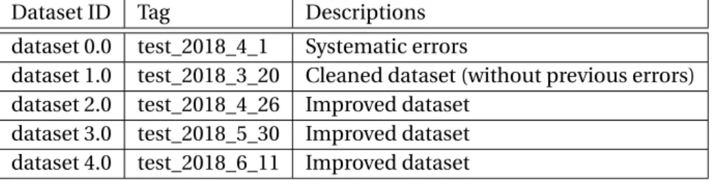
Revisions
Table 1.3 presents the different versions of the dataset. The final dataset contains 1318 obser-vations (555 VPM and 763 no VPM obserobser-vations).
Dataset ID Tag Descriptions
dataset 0.0 test_2018_4_1 Systematic errors
dataset 1.0 test_2018_3_20 Cleaned dataset (without previous errors) dataset 2.0 test_2018_4_26 Improved dataset
dataset 3.0 test_2018_5_30 Improved dataset dataset 4.0 test_2018_6_11 Improved dataset Table 1.3 – Dataset Revisions
2
Related work
Web Classification
Web Classification is a current topic in Machine Learning. The techniques for Web Classifica-tion are derived from Text ClassificaClassifica-tion. The core differences are the following: Unstructured text and noise elements, such as images or javascript [Luca Deri(2015)].
Traditional models can be used for web classification, such as, for instance, N-grams. In the studyTurning Yahoo into an Automatic Web Page Classifier, the author proposes to build feature vectors from web pages (N-grams) to make a classifier [Mladenic(1998)].
In the paper Extracting Search-Focused Key N-Grams for Relevance Ranking in Web Search, the authors find key n-grams (a set of relevant n-grams) from web pages to build relevance rankings [Chen Wang and Cao(2012)].
Summarisation
The paperWeb page Classification through Summarisationshows empirical evidence that Web-page summaries generated by human editors can improve Web-page classification; The authors propose an automatic approach to summarising web content. Summarisation-based classification achieves an improvement of about 8 % [Le(2004)]
Metadata
Metadata information can be used to improve classification rates. There exists several studies that extract features from HTML tags and URL.
Using the Structure of HTML Documents to Improve Retrievalis proposed. This assigns the occurrence of terms into six classes according to the different HTML tags that appear and
weights them according to an importance factor. Information in a H1 HTML tag could be more important than information in H6 HTML tag [Michal Cutler(1997)].
Moreover, studies exist where only the URL is used to classify. In the studyFast Web page Classification using URL features, the authors propose the value of and evaluate different features to classify a web page using only the URL [Kan and Thi(2005)].
3
Techniques
In this section there is a review of different techniques with a view to using them within the project. This includes Text Summarisation, Language Models and Classifiers.
3.1 Web Summarisation
Text Summarisation is an open topic in Natural Language Processing. This technique gen-erates a new text from an existing ones. Likewise, it is possible to make one summary from various texts (Multi Text Summarisation). Extractive and Abstractive models are the two major methods used to make summaries:
Extractive Summarisationis based on identifying important pieces of the text that appear more frequently or in central positions and putting them together build a summary. This method does not preserve the coherence of the output. This method is based on a search of sig-nificant words in the document and on building a word frequency index. The sentences that in-clude these high-frequency words are incorporated in the summary. [Gaikwad and Mahender(2016)] [Luhn(1958)]
Abstractive Summarisationis more challenging than Extractive Summarisation. This tech-nique determines the core sections of the text and builds a novel text with the same meaning. A perfect abstractive summarisation should be humanly readable and undetectable in a pla-giarism check. The actual advances in Deep Learning have enabled more accurate Abstractive methods. For example, the Google Brain project is working in Abstractive Summarisation using Tensor Flow1. [Yogan Jaya Kumar and Suppiah(2016)]
3.2. Language Models
3.2 Language Models
A Language model is a statistical template that explains the probability distribution of nat-ural language. Language Models are commonly used to build and represent a set of words. [Zhang(2012)]
N-gramsis one of the simplest Language models. Given a sequence of N terms, they build sequences of successive terms. A two-term sequence is a bigram, a three-term sequence is a trigram ...[Jurafsky and Martin.(2014)]. Figure 3.3 shows an example of bigrams, trigrams and 4-gram sequences.
Figure 3.1 – Example of a Bigram, Trigram, 4-gram
Skip-Gramsare similar to N-grams. This technique takes a sequence of N terms and allows terms to be skipped. For instance, in the 2-skip-gram of the previous example, "The quick brown fox jumps" are:The quick brown fox jumps, the skip grams are: The quick, The brown, The fox, quick brown, quick fox, quick jump, brown fox, brown jumps and fox jump
TF-IDF(Term Frequency-inverse document frequency). This technique is based on measuring a weight for every term in a set of documents. Words which appears very often in all the docu-ments of the collection have a greater score. [Christopher D. Manning and Schütze(2009)]
Word Embeddingis based on building vector representations of words in a document. This technique puts similar words close in a N-dimensional space [Rong(2016)]
Chapter 3. Techniques
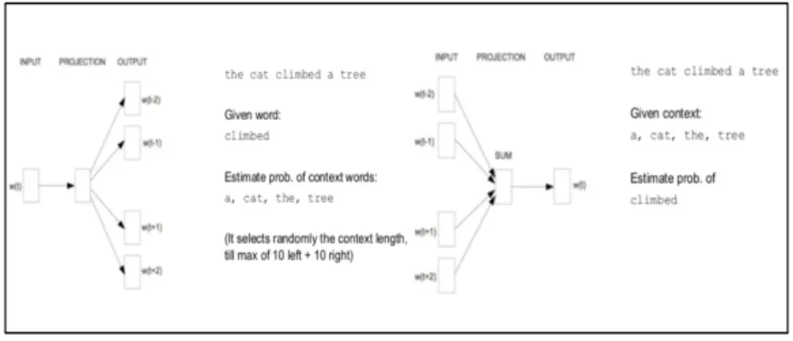
Skip-Grams (SG) and Continuous Bag of Words (CBOW) are the two different models of Word Embedding. Skip-Grams predict surrounding words, given a word. On the other hand, Bag of
words predict words based on context (prediction of surrounding words) [Tomas Mikolov and Dean(2013)].
Figure 3.3 – SG and CBOW examples
Source: D2L4 Deep Learning for Speech and Language UPC 2017, Day 2 Lecture 4, slides 23-24
3.3 Classification
Classification is a common problem in Machine Learning. Classification techniques are based on arranging a set of observations into the same class. The techniques are commonly used, for example, to classify if a user is a candidate for fraudulent behaviour (Market Segmentation), Face Detection (Computer vision) or Spam Filtering (Text Categorization) [Schapire(2008)]. [Ko and Seo(2006)]
Different classification techniques are relevant. The purpose is to use them alongside the project. Included is a short review of Rule-Based Systems, Support Vector Machines, Decision Trees and Extreme Gradient Boosting.
Rule Based Systemsare based on defining a set of rules (IF-ELSE Statements) and filtering the data according to the rules. The main constraint of these systems is the need for human knowledge to define the rules. An example of the application of a Rule-Based System is for the detection of fraudulent online transactions. [Tova Milo and Tan()]
ift r ansac t i on: origin different from client country then ift r ansac t i on: duration > 2hthen
ift r ansac t i on: amount > 5000 CHF then
Possible Fraud Case
Support Vector Machine(popularly known as SVM), is a supervised learning technique. Ob-servations are mapped into an N-Dimensional space, where each observation is set in a
3.3. Classification
specific co-ordinate. This algorithm tries to build a margin (hyperplane) between the different classes. The target of Support Vector Machines is to maximise the width of the margin between classes. Figure 3.4 shows an example of SVM. Here, the red margin splits the data into two classes and misclassified items are controlled with a regularisation parameter (Cparameter).
Figure 3.4 – SVM Example
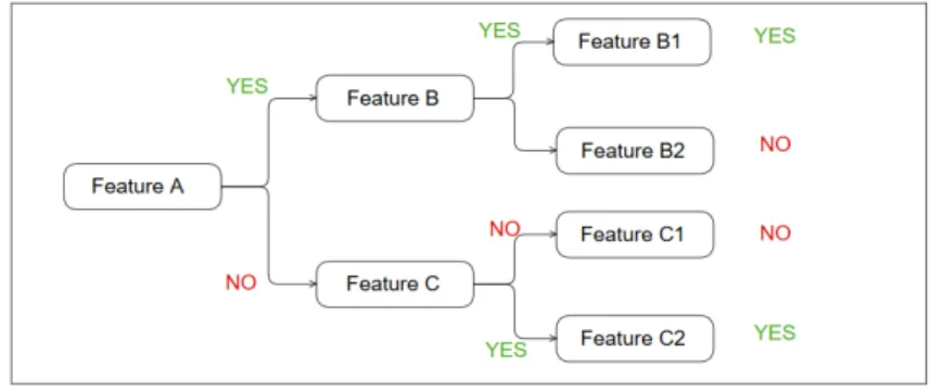
Decision Treesis another supervised technique. This model splits the train data recursively until each partition contains mainly observations of a category. One of the main advantages of this technique is the easy interpretation of the model. (See figure 3.5). Modern Approaches to Decision Trees areRandom-Forestwhich builds a model blending different Decision Trees and where each tree is trained using a random subset of the train data. [quinlan(1986)]
Figure 3.5 – Decision Tree Example
Extreme Gradient BoostingExtreme Gradient Boosting is one of the state of the art classifiers. The algorithm is based in Tree Ensembling. The model builds a set of weak trees and the final prediction is built, merging all previous trees. [Chen(2014)]
4
Proposed work
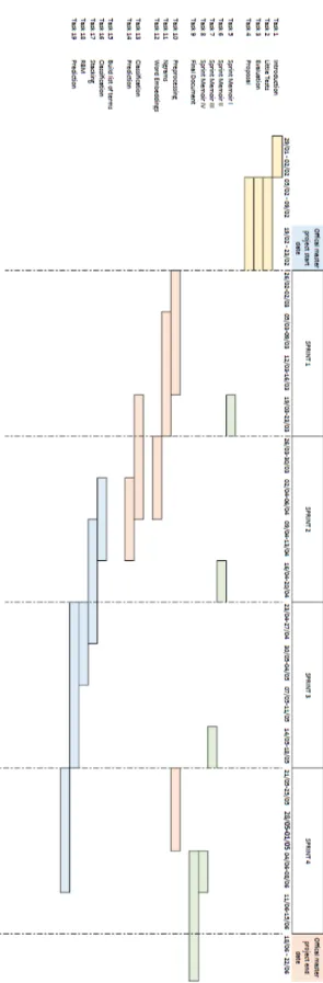
This chapter describes the objectives and methodology (tasks). The methodology section includes the initial Gantt Chart with the work proposed and final Gantt Chart which shows the tasks carried out.
4.1 Objectives
The purpose of IPRoduct project is to build a database of product and patent pairs. As stated in introduction, this contribution to the project is designed to improve the classifier. To this end, the following objectives have been Prescribed.
Objectives:
• Preprocess and extract features from observations. • Classification of VPM pages
• Improve the Labeled Dataset
4.2 Tools
During this project, different machines were used. To begin with the workstation for small tests was utilised, but due to the lack of resources, the work was continued using cdm6-143 server.
•Workstation: 4 cores and 4 GB of memory
4.3. Methodology
4.3 Methodology
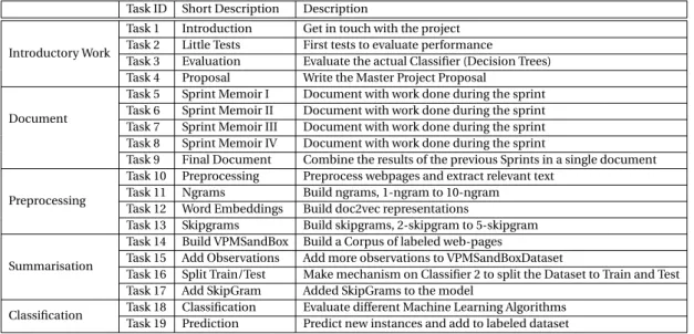
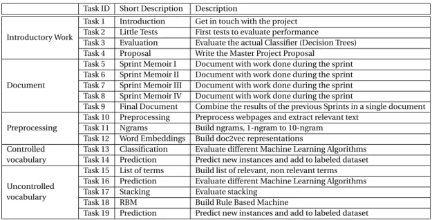
During the project Scrum Methodology was applied. Using an incremental deployment ensured a viable project in a short time. Table 4.1 and 4.1 shows the initial tasks proposed to work in the project. Moving forward, reviewing the tasks with the supervisor of the project, some tasks were changed; Table 4.1 and Figure4.2 show the final task done and the Gantt Chart.
4.3.1 Proposed work
Task ID Short Description Description
Introductory Work
Task 1 Introduction Get in touch with the project Task 2 Little Tests First tests to evaluate performance
Task 3 Evaluation Evaluate the actual Classifier (Decision Trees) Task 4 Proposal Write the Master Project Proposal
Document
Task 5 Sprint Memoir I Document with work done during the sprint Task 6 Sprint Memoir II Document with work done during the sprint Task 7 Sprint Memoir III Document with work done during the sprint Task 8 Sprint Memoir IV Document with work done during the sprint
Task 9 Final Document Combine the results of the previous Sprints in a single document
Preprocessing
Task 10 Preprocessing Preprocess webpages and extract relevant text Task 11 Ngrams Build ngrams, 1-ngram to 10-ngram Task 12 Word Embeddings Build doc2vec representations
Task 13 Skipgrams Build skipgrams, 2-skipgram to 5-skipgram
Summarisation
Task 14 Build VPMSandBox Build a Corpus of labeled web-pages
Task 15 Add Observations Add more observations to VPMSandBoxDataset
Task 16 Split Train/Test Make mechanism on Classifier 2 to split the Dataset to Train and Test Task 17 Add SkipGram Added SkipGrams to the model
Classification Task 18 Classification Evaluate different Machine Learning Algorithms Task 19 Prediction Predict new instances and add to labeled dataset
4.3. Methodology
4.3.2 Work done
Task ID Short Description Description Introductory Work
Task 1 Introduction Get in touch with the project Task 2 Little Tests First tests to evaluate performance
Task 3 Evaluation Evaluate the actual Classifier (Decision Trees) Task 4 Proposal Write the Master Project Proposal
Document
Task 5 Sprint Memoir I Document with work done during the sprint Task 6 Sprint Memoir II Document with work done during the sprint Task 7 Sprint Memoir III Document with work done during the sprint Task 8 Sprint Memoir IV Document with work done during the sprint
Task 9 Final Document Combine the results of the previous Sprints in a single document Preprocessing
Task 10 Preprocessing Preprocess webpages and extract relevant text Task 11 Ngrams Build ngrams, 1-ngram to 10-ngram
Task 12 Word Embeddings Build doc2vec representations Controlled
vocabulary
Task 13 Classification Evaluate different Machine Learning Algorithms Task 14 Prediction Predict new instances and add to labeled dataset Uncontrolled
vocabulary
Task 15 List of terms Build list of relevant, non relevant terms Task 16 Prediction Evaluate different Machine Learning Algorithms Task 17 Stacking Evaluate stacking
Task 18 RBM Build Rule Based Machine
Task 19 Prediction Predict new instances and add to labeled dataset
Chapter 4. Proposed work
5
Preprocessing
In this chapter, the use of preprocessing is explained. The purpose of using preprocessing is to reduce the noise of the observations and to improve the quality of the dataset. Preprocessing is applied to uncontrolled and controlled vocabulary approaches deployed during the project. As already stated in Introductory chapter web pages contain a lot of irrelevant information such as Images, Metadata or JavaScript. Removing these elements make it possible to improve Data quality.
Data quality covers several data factors. This includes the accuracy, precision, completeness, consistency, timeliness, believability and interpretability [Jiawei Han and Pei(2012)]. In this case with the application of preprocessing it aims to enhance the accuracy and precision of the dataset.
During this stage,two different data preprocessing techniques were applied: Data Cleaning and Data Normalisation. Data Cleaning works to remove irrelevant or noisy information from the study. On the other hand, Data Normalization refers to the adjustment of values to a common scale.
Figure 5.1 includes an example of a real webpage (left side) and the web page after prepro-cessing (right side) where relevant aspects of the web page are captured for further analysis (highlighted in yellow).
Chapter 5. Preprocessing
Figure 5.1 – From left to right: Original website and selected fractions with relevant information Original: https://www.top
gear.com/car-news/electric/everything-you-need-know-about-cars-week-20-April-20181
Figure 5.2 is a diagram of the different tasks of preprocessing. The source of data is raw text (in the case of Labeled Dataset). In the evaluation stage, there are no seen observations as the observations are stored in Warc files.
A WARC file is a container of web pages. Each web page stores the raw text and metadata (time stamp). To read and write files special libraries are needed. During the project, Warcio a python 3.2 library, was used. Warcio offers high-level functions to read and write WARC files.
• Parsing.This refers to the removal of irrelevant tokens from the websites such as Images, JavaScripts, URL etc. To perform this task a html2text package is used. This library automatically detects and deletes irrelevant tokens.1
• Patent Detection. Here, a regex function is used to detect patent numbers on the web page. For example, in this phase, the detected numbers (for example US7,123,777, US Patent 8,726,186 or US6563491) were replaced with ’patent number’ item.
• Tokenisation. In this stage, every relevant word in the study is tokenised. This technique is based on splitting the previous plain-text into tokens according to white spaces or special characters such as "?", ";" or ",". For example "The quick brown fox jumps over the lazy dog" is tokenised into : "the", "quick", "brown", "fox", "jumps", "over", "the", "lazy", "dog". Through the project the word_tokenise function is used as taken from nltk library.
• Stopword Removal. . Stopwords are high-frequency words that add coherence to the text. By removing these stopwords it is possible to reduce the complexity of the classifier. For the purpose of the study All stop words were removed Deleting the stopwords such asand, or, the, an ..., a total of 211 different items were taken into account. From the previous example it was demonstrated that by deleting from the item "the"; the resulting string is : "quick", "brown", "fox", "jumps", "over", "lazy", "dog"
• Canonicalisation:With Canonicalisation every word is reduced to a common form. The aim of canonicalisation is to diminish the corpus to analyse. There exists two main techniques of canonicalisation: Stemming and Lemmatizing.
Stemming is a heuristic approach that chops off the end of the word in order to reduce derivation affixes. For example, the word ’studies’ is reduced to studi (suffix -es). On the other hand, Lemmatizing reduces each word to the lemma (cannonical form of the word; the word which appears in the dictionary). This technique is based on the morphological analysis of each , but time and resources are consuming with this approach. With Lemmatizing the word ’studies’ is reduced to study.
During this project it was decided that the use of Stemming and Lemmatizing offers a more accurate canonicalisation of words, but is slower. To perform Stemming the Porter Stemmer algorithm was implemented on nltk package.
6
Uncontrolled Vocabulary
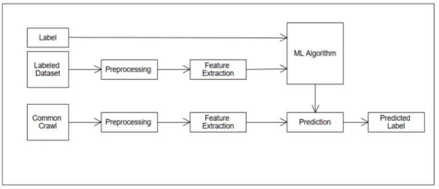
In this section, the first attempts to develop a classifier are explained. Feature vectors are built using n-grams and word embeddings; The previous feature vectors are classified us-ing different classifiers includus-ing Random Forests, Support Vector Machines and XGBoost classifiers.
Having found the best model, this was then used to predict Common Crawl instances (non-seen observations). Figure 6.1 shows a schema of the first approach.
Figure 6.1 – First Approach Framework Adapted from https://www.analyticsvidhya.com/
Building and testing this model helps to develop a better understanding of the dataset. Using this approach, key n-grams are selected and extracted. This gives insight into Virtual Patent Marking Information. Key n-grams are used during second approach developed in this project.
6.0.1 Experiments
First of all, web pages are preprocessed applying the preprocessing steps previously defined (see Preprocessing section). Each web page contains build feature vectors using n-grams
(1-gram up to 8-(1-gram) and DOC2VECs (with the following configuration: alpha_val=0.02, Initial learning rate; min_alpha_val=1e-4 and passes=15, number of epochs during the training). In this section there is an evaluation of the performance of three classification algorithms. All the results shown in this section have been demonstrated using 10-fold cross validation and Hyperparameter optimisation (using GridSearchCV). Table 6.1 includes the parameters tuned. The implementation of SVM and Random Forest is included in Sci-kit library. On the other hand, XGBoost is available in dmlc/xgboost repository.1 2
Algorithm Tested features
SVM C and Kernel
Random Forests max_depth and n_estimators
XGBoost min_child_weight, max_depth, gamma,
col-sample_bytree, subsample, reg_alpha, learn-ing_rate
Table 6.1 – Hyperparameter Optimization parameters
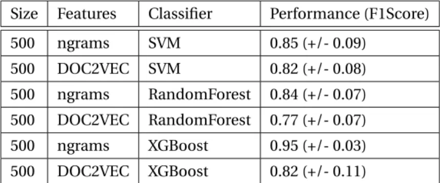
Tables 6.2, 6.3, 6.4 and 6.5 presents the results of varying the dataset size from 50 up to 500, the features and the classifier. To evaluate the performance F1-Score and the Confidence Interval are included.
Size Features Classifier Performance (F1Score)
50 ngrams SVM 0.69 (+/- 0.40) 50 DOC2VEC SVM 0.76 (+/- 0.45) 50 ngrams RandomForest 0.80 (+/- 0.32) 50 DOC2VEC RandomForest 0.70 (+/- 0.45) 50 ngrams XGBoost 0.89 (+/- 0.37) 50 DOC2VEC XGBoost 0.76 (+/- 0.39)
Table 6.2 – Results for size 50
1Scikit Library : http://scikit-learn.org/stable/index.html 2XGBoost Repository : https://github.com/dmlc/xgboost
Chapter 6. Uncontrolled Vocabulary
Size Features Classifier Performance (F1Score)
100 ngrams SVM 0.77 (+/- 0.25) 100 DOC2VEC SVM 0.79 (+/- 0.20) 100 ngrams RandomForest 0.80 (+/- 0.32) 100 DOC2VEC RandomForest 0.79 (+/- 0.88) 100 ngrams XGBoost 0.97 (+/- 0.10) 100 DOC2VEC XGBoost 0.75 (+/- 0.13)
Table 6.3 – Results for size 100
Size Features Classifier Performance (F1Score)
250 ngrams SVM 0.78 (+/- 0.23) 250 DOC2VEC SVM 0.80 (+/- 0.22) 250 ngrams RandomForest 0.83 (+/- 0.15) 250 DOC2VEC RandomForest 0.63 (+/- 0.20) 250 ngrams XGBoost 0.96 (+/- 0.05) 250 DOC2VEC XGBoost 0.77 (+/- 0.21)
Table 6.4 – Results for size 250
Size Features Classifier Performance (F1Score)
500 ngrams SVM 0.85 (+/- 0.09) 500 DOC2VEC SVM 0.82 (+/- 0.08) 500 ngrams RandomForest 0.84 (+/- 0.07) 500 DOC2VEC RandomForest 0.77 (+/- 0.07) 500 ngrams XGBoost 0.95 (+/- 0.03) 500 DOC2VEC XGBoost 0.82 (+/- 0.11)
Table 6.5 – Results for size 500
Using the previous tables, it was found that working with XGBoost gives very reliable results. Working with a dataset of 500 Observations (250 VPM and 250 no VPM web pages) an F1-Score of 0.95 is achieved. However, intuitively it was assessed that this result can be biased due the small sample of observations. Therefore, to train a model with more observations was attempted but with the actual server (cdm6-143) it was seen to have an memory error.
6.0.2 Analysis of observations
In this section, the output of XGBoost is analysed as the classifier with the best performance. Figures 6.4, 6.2, 6.3 are commonly used to interpret XGBoost results. Gain is the contribution of each feature (n-grams) to the model calculated. Cover explains the number of appearances related to this feature. Finally, weight is the relative number of times a particular feature occurs in trees.
Figure 6.2 – Gain : average gain of the feature
Figure 6.3 – Cover : average coverage of the feature
Chapter 6. Uncontrolled Vocabulary
As can be see from previous plots most of the n-grams that contribute to the model are not indicators of VPM information. For example, the term ’year’, ’11’ and ’file (the n-grams with more Gain) can occur in both types of web pages. On the other hand, if a web page contains the term ’claim’ or ’infrig’it is more likely to be VPM.
Table 6.6 shows the relevant n-grams used by XGBoost to build decision trees. The n-grams are grouped into 5 categories.These categories refer to VPM Relevant n-grams relating to VPM information, VPM Non-Relevant (news) and VPM Non-Relevant (lawsuit) as n-grams related to news and lawsuit websites. Finally, Non-Relevant and Bad preprocessing are noisy n-grams.
Category Terms (n-grams)
VPM Relevant infring , expir , protocol , right reserv , otherwis provid , ip , pend , dis-trict court , copyright , reliabl , patentnumb patentnumb patentnumb , patentnumb patentnumb , patent pend , patent infring , infring , protect one , list , accord patent, marking, protection, legal,claim state-ment, and usa
VPM Non Relevant (news)
articl , rss , tweet , news , articl , archiv, document, press , file , comment and cart
VPM Non Relevant (lawsuit)
litig , citat, issu , court, lawsuit , membership , prototyp, district , attorney and law
Non Relevant crystal , accept , particip , music , understand , year , de , cloud , side effect, identifi, coupl, enough, chicago, activ, civil, confirm, free, alreadi , contact us , watch , recent , secret , rel , result , public , manag , warranti , websit , season , career , facebook , avoid , comment, north carolina, compli , est , updat , technolog , statutori , separ , addit, delawar , end , arriv , appl , make , noth , qualiti , push , plan , use , none , month , maximum , custom , yet , sell , fair , otherwis , solut , gener , store , 6 , discontinu , latest , train , employ , user and date Bad preprocessing 0 , _blank , 06 , 007, 5, http, link , 30 , st , et , ga , display none , top ,
properti, valid and top
Table 6.6 – Relevant terms
From table 6.6 it can be seen that most of the featured n-grams used by XGBoost are not good indicators (Non-Relevant and Bad prepossessing). The n-grams are tagged as bad indicators because these terms can be in a VPM or no VPM web page. On the other hand, if a web page contains the terms of a VPM Relevant category it is more probable that the web page is a VPM web page.
Next, all the branches of an XGBoost execution were ranked( this includes first 20 occurrences). Every branch contributes to the ensembles model which is the sum of all boosted trees in the model. From previous output some interesting branches were found. For example, the top three branches includes the n-grams ’court’, ’claim’ and ’litig,’ but also includes noisy n-grams such as : ’12 month’, ’15’ or ’mean’.
Id Contibution Branch
1 0.0194406 ’court’ < 1 & ’12 month’ < 1
2 0.0192596 ’litig’ < 1 & ’membership’ < 1 & ’mean’ < 2 3 0.0190548 ’court’ < 1 & ’15’ < 4
4 0.0190361 ’litig’ < 1 & ’membership’ < 1 & ’claim’ < 2 5 0.0188329 ’claim’ < 2 & ’10’ < 7 & ’district’ < 1 6 0.0186913 ’court’ < 1 & ’citat’ < 1 & ’2007’ < 1 7 0.0183851 ’litig’ < 1 & ’membership’ < 1 & ’claim’ < 2 8 0.0182198 ’court’ < 1 & ’summari’ < 1
9 0.0182017 ’court’ < 1 & ’citat’ < 1 10 0.0179179 ’court’ < 1 & ’app link’ < 1 11 0.0179132 ’court’ < 1 & ’account today’ < 1 12 0.0176294 ’litig’ < 1 & ’95’ < 5 & ’claim’ < 2 13 0.0174944 ’court’ < 1 & ’summari’ < 1
14 0.0174788 ’prosecut’ < 1 & ’court’ < 3 & ’claim’ < 2 15 0.0173753 ’litig’ < 1 & ’membership’ < 1 & ’claim’ < 2 16 0.0174788 ’prosecut’ < 1 & ’court’ < 3 & ’claim’ < 2 17 0.0173753 ’litig’ < 1 & ’membership’ < 1 & ’claim’ < 2 18 0.0171013 ’court’ < 1 & ’summari’ < 1
19 0.0170933 ’court’ < 1 & ’citat’ < 1
20 0.0166436 ’claim’ < 2 & ’patent search’ < 1 & ’851’ < 2
6.0.3 Evaluation
After ascertaining the best model, Common Craw was used to predict observations. A small test was run and a prediction of a sub-set of observations made (10,550 observations). The model predicts 54 True cases and 10496 False cases. After manually reviewing the True cases it was identified that only 7 web pages where VPM pages.
Chapter 6. Uncontrolled Vocabulary
6.0.4 Conclusion
This model is based on use language models and classification algorithms. As seen in 6.0.1 the configuration XGBoost+ngrams shows promising results (an F1-Score of 0.95). However, during prediction, it was found that performance is lowest. One of the reasons is the small sample used. It is suspected that the dataset is not representative and, therefore the interesting observations are not included in the training data.
7
Controlled Vocabulary
The main purpose of building a different approach is to build a model, less complex and to be able to predict observations from Common Crawl faster. The previous approach takes too much time to build Feature Vectors. One of the novelties of this approach is to use a list of relevant and non-relevant n’grams (part of these n’grams included in the list found in the previous section) and used to infer this knowledge to the classifier. Moreover, it can be included in the analysis of metadata to improve classification. Figure 7.1 shows the procedure of Controlled Vocabulary approach.
Figure 7.1 – Second Approach Framework Adapted from https://www.analyticsvidhya.com/
7.0.1 Key n-grams
In the last chapter, the n-grams were categorised as relevant or not relevant(see table 6.6). The purpose is to build a list of relevant and non-relevant n-grams to use as features of the classifier. To look for more key n-grams two tasks are then performed: sort N-grams and look for synonyms. The objective is to build a classifier only with n-grams that are believed to be relevant.
Chapter 7. Controlled Vocabulary
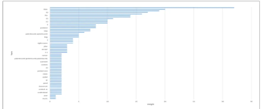
Sort N-gramsAll the n-grams of the Labeled Dataset (True VPM Observations)are manually rank by frequency. This helps to identify frequent n-grams not captured by XGBoost. The appendix B: Ngram Frequencies includes an histogram with top 100 n-grams.
Look for synonymsUsing the tool Semantic pipeline synonyms of relevant terms highlighted by XGBoost are identified. This tool uses word embeddings (glove algorithm) to search similar terms in a corpus of documents.1
Figure 7.2 – ’Patent’ and ’Lawsuit’ similar terms
Figure 7.2 shows similar items to patent and lawsuit. For example ’trademark’, ’infrigment’ and ’invention’ are the most similar items to patent. The cases where one synonym is shared between two disjoint classes (patent and lawsuit or patent and news) they are classified according to current knowledge. In the case of the ’claim’ n-gram, they are classified as relevant n-gram.
Tables 7.1 and 7.5 show the two lists built with examples of selected grams. Also, the n-grams are grouped into different categories. The purpose is to perform a more fine-grained classification using these categories but this is probably beyond the scope of this project.
Concepts N. of items N-grams
legal statement 100 product servic, patent may pend, claim list
license 12 licens agreement, exclus licens, patent licens
marking 29 patent mark, virtual patent, 287
other_ip 13 intellectu properti, regist trademark
patent 37 unit state patent, patent pend, patent no
protection 37 protect one, product protect, protect patent
USPTO 3 trademark offic, patent trademark offic,
uspto
Table 7.1 – Relevant ngrams
Category N. of items N-grams
news 24 headlin, podcast, report, today, archiv, press,
forum ...
lawsuit 13 sue, class-act, litig, alleg, attorney ...
court 13 judg, suprem, appeal ,rule ,judici ...
Table 7.2 – Non-relevant ngrams
7.0.2 Metadata
In literature, several studies can be found that conclude that a proper analysis of metadata can improve classification rates (see section State-of-the Art). In this project the analysis of the URL, Title, Description and Content is introduced. Figures 7.3 include the different dimensions used in the study.
Features Description
URL(n-grams) VPM relevant ngrams in URL
Depth Count of "/" in the URL
Length Length of the URL
Title VPM relevant ngrams in Title
Description(Metadata) VPM relevant ngrams in description
Keywords(Metadata) VPM relevant ngrams in keywords
Table 7.3 – Metadata dimensions
Chapter 7. Controlled Vocabulary
analysis can work for the project:
Title (metadata) BBC - Homepage
Description (metadata) Breaking news, sport, TV, radio and a whole lot more. The BBC informs, educates and entertains - wherever you are, whatever your age
Keywords (metadata) BBC, bbc.co.uk, bbc.com, Search, British Broadcasting Cor-poration, BBC iPlayer, BBCi
URL (after parsing) bbc
Table 7.4 –https://bbc.com(a false positive case)
Title (metadata) Virtual Patent Marking | Outbrain.com
Description (metadata) Outbrain products are protected by patents in the U.S. and elsewhere. See this webpage for the virtual patent marking provisions of various jurisdictions
Keywords (metadata)
-URL (after parsing) outbrain, patent
Table 7.5 –https://www.outbrain.com/patents/(a true positive case)
It can be seen in the second example:https://www.outbrain.com/patents/the Title, URL and Description contain relevant n-grams.
7.0.3 Domain Check
During prediction, the domain of the web age is checked. The aim of domain checker is not predict web ages from domains where we know is no vpm information. For example, the domainpatents.google.comcontains web pages where the classifier could easily classify as a false positive. This domain contains lot of descriptions of patents and the classifier can easily tag a VPM web page.
A list of non-relevant domains is manually built. To build the filter a list of 2290 domains is used. This list is built taking all domains from common crawl and ranking the number of pages per domain.
The list comprises many features including search engines (google.com, google.nl, yahoo.com, ...) news and articles domains (wordpress.com, cnet.com, wikisource.org, ...) and also domains about patent news or lawsuit articles (patentados.com, freshpatents.com, freepatentson-line.com, ...)
7.0.4 Classification
Table 7.6 shows the performance of different algorithms using different sets of features (listed below). For each experiment a hyperparameter optimization was used and 10-fold cross-validation.
• URL: relevant ngrams in URL, Depth and Length
• Metadata: relevant ngrams in Description and Keywords • Relevant: relevant ngrams in body
• Non-Relevant: non relevant ngrams in body
Features Algorithm Performance (F1Score)
URL Random Forest 0.76 (+/- 0.10)
URL SVM 0.76 (+/- 0.11)
URL XGBoost 0.74(+/- 0.05)
Metadata Random Forest 0.53 (+/- 0.20)
Metadata SVM 0.65 (+/- 0.28)
Metadata XGBoost 0.74 (+/- 0.05)
URL + Metadata Random Forest 0.58 (+/- 0.29)
URL + Metadata SVM 0.81 (+/- 0.11)
URL + Metadata XGBoost 0.78 (+/- 0.16)
Relevant Random Forest 0.71 (+/- 0.33)
Relevant SVM 0.85 (+/- 0.20)
Relevant XGBoost 0.87 (+/- 0.21)
Non-Relevant Random Forest 0.77 (+/- 0.19)
Non-Relevant SVM 0.82 (+/- 0.19)
Non-Relevant XGBoost 0.79 (+/- 0.27)
Relevant + Non-Relevant Random Forest 0.80 (+/- 0.21)
Relevant + Non-Relevant SVM 0.87 (+/- 0.19)
Relevant + Non-Relevant XGBoost 0.88 (+/- 0.21)
Relevant + Non-Relevant + URL + Metadata Random Forest 0.86 (+/- 0.11)
Relevant + Non-Relevant + URL + Metadata SVM 0.88 (+/- 0.11)
Relevant + Non-Relevant + URL + Metadata XGBoost 0.89 (+/- 0.16)
Chapter 7. Controlled Vocabulary
First of all, it was found that in analyzing the URL a F1-Score of 0.76 (+/- 0.10) is obtained. This is a very significant result given that it was only based on looking at the URL of the web page without looking inside the web page (very fast classifier). Adding the metadata features the model is improved to 0.078 .
Working with the list of key n-grams (relevant and non-relevant) shows good performance: 0.88 (+/- 0.21), complete analysis of the web age Furthermore, these results are improved when adding URL+Metadata dimensions to 0.89 (+/- 0.16). In this case by adding URL + Metadata features the confidence interval is reduced (better model).
Table 7.3, 7.4 and 7.5 shows Gain, Cover and Weight for best xgboost model found previously (Relevant + Non-Relevant + URL + Metadata). The three features with more gain are the following : ’addit patnet may’ and ’post’ ngrams and the length of the url.
Figure 7.3 – Gain : average gain of the feature
Figure 7.4 – Cover : average coverage of the feature
Chapter 7. Controlled Vocabulary
The next step is to include the branches built by XGBoost, as referred to in the Uncontrolled vocabulary section:
1 0.0186505 ’length_url’ < 57 & ’patent metadata’ >= 1,
’attorney count_non_relevant’ < 2 2 0.0186325 ’court count_non_relevant’ < 1,
’patent metadata’ >= 1,
’daili count_non_relevant’ < 1,
’patentnumb count_relevant’ >= 1,
’may cover count_relevant’ < 1,
’articl count_non_relevant’ < 1 3 -0.0184375 ’court count_non_relevant’ >= 1,
’intellectu properti right count_relevant’ < 3 4 -0.018416 ’length_url’ >= 51,
’addit patent may count_relevant’ < 1,
’provid satisfi virtual count_relevant’ < 1,
’section 287 count_relevant’ < 1, ’law count_non_relevant’ >= 1 5 0.0179537 ’length_url’ < 51, ’patent metadata’ >= 1, ’today count_non_relevant’ < 1 6 0.0177919 ’length_url’ < 57, ’patent metadata’ >= 1, ’daili count_non_relevant’ < 1, ’patentnumb count_relevant’ >= 1 7 0.0176858 ’length_url’ < 55, ’patent metadata’ >= 1, ’attorney count_non_relevant’ < 2 8 -0.0172423 ’length_url’ >= 51,
’provid satisfi virtual count_relevant’ < 1,
9 0.0171612 ’length_url’ < 51, ’patent metadata’ >= 1, ’today count_non_relevant’ < 1 10 0.017018 ’length_url’ < 56, ’patent metadata’ >= 1, ’attorney count_non_relevant’ < 2 11 0.0169353 ’length_url’ < 57, ’patent metadata’ >= 1, ’today count_non_relevant’ < 2, ’archiv count_non_relevant’ < 1 12 -0.0169349 ’length_url’ >= 56, ’patentnumb count_relevant’ < 4,
’product code count_relevant’ < 1,
’provid satisfi virtual count_relevant’ < 1,
’regist trademark count_relevant’ < 2
Inspecting previous plots of gain, cover and weight and rules it was found that the length of the URL is one of the most relevant dimensions. Web pages with length less than 55 characters are more likely to contain virtual patent marking information. After analysing manually the URL of the web pages it was found that, in fact, it may make sense that most of the VPM pages are corporative pages where the URL is built only with the name of the company as for instance : https://www.360fly.com/patents or http://cscpatents.com/.
Rule Based Machine
In this section an evaluation of the performance to classify the Labeled Dataset using a Rule Based Machine takes place. The rules are defined according to the output of XGBoost, the branches with more contribution to the final model are selected and they are used to filter instances.An F1-Score of0.689is obtained. This result is lower than using a list of key n-grams and stacking.
Stacking
To further improve classifications rates Stacking is tested. Stacking is an Ensemble algorithm. This technique uses the prediction of several machine learning algorithms (commonly named as base-learner) and a meta-learner to give a prediction based on the individual learners.
Chapter 7. Controlled Vocabulary
In this section, Random Forest, SVM, XGBoost, LightGBM and Catboost as Base learners and XGBoost as meta-learner are all tested.
Xgboost, Catboost and LightGBM are three different state-of-the-art gradient boosting im-plementations. LightGBM as developed by Microsoft in 2017 is an algorithm that introduces Gradient-based One-Side Sampling (Gos) to select the best split. On the other hand, Cat-boost was developed by Yandex in 2017 and introduced two novelties to Cat-boosting: ordered boosting and an innovative algorithm for deal with categorical features. Table 7.7 includes the result of stacking using different features and different base learners. All experiments are done using Hyperparameter Optimization and 10 fold cross-validation. For each test an F1-Score and the improvement using stacking (see table 7.6) are included. [Swalin(2018)] [Liudmila Prokhorenkova and Gulin(2017)]
Features Base Learner Meta
Learner
F1-Score Imp.
Relevant Random Forest, SVM,
XG-Boost
XGBoost 0.82 +/-0.02 0.01
Relevant + Non Relevant Random Forest, SVM, XG-Boost
XGBoost 0.88 +/-0.06 0
Relevant + Non Relevant + URL
Random Forest, SVM, XG-Boost
XGBoost 0.88 +/-0.05 -0.01
Relevant Random Forest, SVM,
XG-Boost, LightGBM, Cat-Boost
XGBoost 0.83 +/-0.02 -0.04
Relevant + Non Relevant Random Forest, SVM, XG-Boost, LightGBM, Cat-Boost
XGBoost 0.89 +/-0.02 0.01
Relevant + Non Relevant + URL + Metadata
Random Forest, SVM, XG-Boost, LightGBM, Cat-Boost
XGBoost 0.93 +/-0.02 0.04
Table 7.7 – Stacking
As can be seen, using stacking, the results improve from 0.89 to 0.93. The improvement using Stacking is of 0.04 using 5 different Base Learners. However, the main issue with Stacking is that it is a more complex model and difficult to interpret.
8
Improving Dataset
One of the tasks of this project is to improve the Labeled dataset. In this section, a methodology is defined to systematically improve the dataset. The purpose is of this task is to achieve a representative dataset of VPM observations. This dataset is essential to improve and train a competent classifier. In this section, the process of increasing the dataset from 400 to 1300 observations is explained.
Procedure
The following procedure is used to add new observations:
• 0a. select one of the models
• 0b. select which type of vpm pages need to be detected (svpm, or svpm+hvpm+cvpm+ovpm, or other).
• 1. train the model on the current training dataset
• 2. run it on "commoncrawl filter1" (or a part of it)
• 3. Manually check vpm observations and classify them over the 5 cases (svpm, hvpm, cvpm, ovpm, and no-vpm) **
** To manually check and classify the observations the probability of being VPM is predicted and the first 200 observations of each segment are sorted and checked manually (The common crawl is divided into 10 segments).
Chapter 8. Improving Dataset
Revisions of the dataset
In this section it is explained how the dataset is incrementally improved. The first version is a dataset previously built by IPRoduct team and a dataset 1.0 with some systematic errors remedied (such as error 404, or web page not found websites). The following 2 iterations are done applying the procedure and the final iteration adds all the misclassified items found in previous iterations.
Dataset 0.0, test_2018_4_1Initial Dataset, this dataset is not split into the six categories defined in this document (see table 1.2). This revision is used only to get into the project.
• Categories: True Cases : vpm pages and False Cases : no-vpm pages • Total webpages: VPM pages (403) and no VPM pages (403)
Dataset 1.0, test_2018_4_20In this revision are fixed systematic errors of Dataset 0.0, This dataset was used during the first test in Uncontrolled vocabulary approach. During this revision is introduced the six categories dataset VPM : svpm, ovpm, cvpm and noVPM : news, lawsuit and other.
• Categories: True Cases : svpm+hvpm+cvpm+ovpm and False Cases : news+lawsuit+other • Total web pages, fixing systematic errors: VPM pages (svpm : 380 observations, ovpm :
5 observations and cvpm : 22 observations) and no VPM pages (lawsuit : 73 observations, news : 192 observations, other : 70 observations)
Dataset 2.0, test_2018_4_26In this revision the procedure defined was applied. A prediction and check of five segments of Common Crawl is conducted. 100 observations are added to the dataset. Half of the web pages are VPM (including some no VPM web pages to balance the dataset). To predict web pages XGBoost (best model found in Controlled Vocabulary) is used.
• Dataset: True Cases : svpm+hvpm+cvpm+ovpm and False Cases : news+lawsuit+other • : VPM pages (svpm : 419 observations, ovpm : 11 observations and cvpm : 80
observa-tions) and no VPM pages (lawsuit : 81 observations, news : 294 observations, other : 126 observations)
Dataset 3.0, test_2018_5_30In this revision the procedure is applied, during this stage, also including the domain filter. In this revision 269 new observations are added to the dataset. Half of the web pages are VPM (some no VPM web pages are included to balance the dataset). To predict web pages, XGBoost (best model found in Controlled Vocabulary)is used.
• Dataset: True Cases : svpm+hvpm+cvpm+ovpm and False Cases : news+lawsuit+other • Total web pages, after adding new observations: VPM pages (svpm : 440 observations, ovpm : 11 observations and cvpm : 93 observations) and no VPM pages (lawsuit : 81 observations, news : 294 observations, other : 192 observations)
Moreover, in an attempt to understand misclassified items, some examples of these web pages are listed:
- http://moderustic.com/Outdoor-Fireplaces.html [COMPLEX PAGE], predicted True but False. To many relevant n-grams like ’patent’, ’patent pending status’ and without non-relevant ngrams.
- https://www.eharmony.com/ca/ [COMPLEX PAGE], predicted False but True. Only appear the n-gram ’protected by’
- http://roohit.com/collection/index.php?what=tagtag=%27Release%27.html [COMPLEX PAGE], predicted False but True. Only appears the n-grams: ’patent’ and ’patent pending’
- https://hedgeconnection.com/blog/?p=2289.html [COMPLEX PAGE], predicted False but True. Only appears the n-gram ’patent’
Dataset 4.0, test_2018_6_11In this revision we include mis-classified items to the dataset (False Cases). A total of 504 observations are added. This revision of the dataset is not balanced.
• Dataset: True Cases : svpm+hvpm+cvpm+ovpm and False Cases : news+lawsuit+other • Total web pages, after adding new observations: VPM pages (svpm : 440 observations, ovpm : 11 observations and cvpm : 93 observations) and no VPM pages (lawsuit : 326 observations, news : 353 observations, other : 326 observations)
Chapter 8. Improving Dataset
Next, an example is included of how to improve the prediction by adding more observations to the labelled dataset. In table 8.1 it can be seen that the number of pages correctly tagged (only 200 first occurrences were reviewed) from two segments of common crawl (RDD 0 and RDD 1). In the First prediction, the Dataset 1.0 was used and in second iteration Dataset 2.0 was used. Dataset 2.0 includes the VPM observations found in the first prediction.
RDD Total Pages Filtered Tagged first iteration Tagged, second iteration
RDD 0 152163 14/200 54/200
RDD 1 384000 24/200 44/200
Table 8.1 – Evaluation first iteration
As can seen, using the using an improved dataset to do the predictions means detecting more VPM web pages. Using Dataset 2.0 a higher number of VPM pages can be detected. As for instance. in RDD 0, 40 new web pages are identified .
9
Conclusions
In this project, different procedures for Web Classification were analyzed. During the research, web pages were classified according to whether they had VPM information or not. This task was not trivial, as observed during the project. Several web pages only include small insights that give intuitions to how to tag the web page.
During the project, an appropriate preprocessing was found to be highly important.Here, it is suggested that one possible area of future work that would probably be advantageous, would be to keep working on a better-preprocessing stage.
In the first model, Controlled vocabulary, a traditional approach was reviewed involving ngrams and word embeddings. When a large dataset is trained (not enough representative of the whole dataset) in cdm6 server it is observed to have a memory error. This memory limitation is one reason to find a more simple model. To keep working in this approach more resources are needed or it is necessary to migrate to a bigger machine.
In the final approach, Controlled vocabulary, a list of relevant and non-relevant n-grams and Metadata analysis are inferred to the classifier. Using this approach it is possible to achieve a similar but working with a less complex model.
To keep developing this project, once the nature of data (not an easy dataset) is known, the best option might be to work on improving Metadata features and Meta-analysis. It was found that by adding metadata features classification rates are improved. Next, several options to keep improving this project are included.
Chapter 9. Conclusions
9.0.1 Future Work
This project was developed as a masters’ thesis, as a five-month project. Since this time frame was not sufficient to test all the ideas and proposals initiated, there is now included a list of proposals to move forward with the project.
Word Embeddings, In the initial approach, the attempt to develop this aspect of the work resulted in limitationsdoc2vecand was without further results other than using n-grams (a simpler approach). Probably tuning doc2vec or applying similar techniques such as sentence vector (different granularity) would enhance classification rates. [Le(2014)]
Meta-analysisDuring Controlled Vocabulary section, metadata information was introduced (Relevant n-grams at metadata) with good results. As pointed out in Related work section, there exists studies that can prove that weighting the content on HTML tags according to their importance can improve classification rates. Including this outline could improve classifica-tion. Moreover looking for HTML tags could be a worthwhile improvement as most of the home vpm pages show patent information at the end of the web page.
SummarisationSummarisation was one of the tasks proposed to improve the classifier. Due to limited knowledge of the nature of VPM web pages, this has not been implemented. However, having reached a strong understanding of how VPM appears in web pages it is possible to consider re-investigating this work.
Multinomnial ClassifierObservations are classified into six groups(see table 1.2) but this fine-grained study does not take into account in this project. During the project, group svpm,hvpm and ovpm were defined as True VPM and news, lawsuit and other as False VPM observations. One interesting task is to work with a Multinominal classifier and try to classify instances in the six categories described previously.
A
VPM examples
In this section is included graphical examples of the different types of webpages with Virtual Patent Marking pages. The first type of webpages (Classified as simple complexity webpage) is the VPM Page (svpm) Figure A.1. Examples of Complex VPM are included in Figure A.2 and Figure A.3 (hvpm and ovpm). Finally Figure A.6 is an example of a Non VPM Page
Appendix A. VPM examples
Figure A.2 – HVPM Page: VPM Home page
Figure A.4 – NVPM Page: news
Appendix A. VPM examples
Appendix B. Ngram Frequencies
B
Ngram Frequencies
Bibliography
[Chen(2014)] Tianqi Chen. Introduction to boosted trees. 2014.
[Chen Wang and Cao(2012)] Yunhua Hu Hang Li Chen Wang, Keping Bi and Guihong Cao. Extracting search-focused key n-grams for relevance ranking in web search.WSDM’12, 2012.
[Christopher D. Manning and Schütze(2009)] Prabhakar Raghavan Christopher D. Manning and Hinrich Schütze. Introduction to information retrieval.ISBN: 0521865719, 2009.
[Courtois(2017)] Jules Courtois. Iproduct : Product name identification. 2017.
[E. Orliac(2017)] G. Fourestey E. Orliac. Patent-crawler, a real-time recursive focused web crawler to gather information on patent usage. 2017.
[Gaikwad and Mahender(2016)] Deepali K. Gaikwad and C. Namrata Mahender. A review paper on text summarization. International Journal of Advanced Research in Computer and Communication Engineering, 2016.
[Jiawei Han and Pei(2012)] Micheline Kamber Jiawei Han and Jian Pei. data mining concepts and techniques.ISBN: 978-0-12-381479-1, 2012.
[Jurafsky and Martin.(2014)] Daniel Jurafsky and James H. Martin. Speech and language processing.International Journal of Advanced Research in Computer and Communication Engineering, 2014.
[Kan and Thi(2005)] Min-Yen Kan and Hoang Oanh Nguyen Thi. Fast webpage classification using url features. CIKM, 2005.
[Ko and Seo(2006)] Youngjoong Ko and Jungyun Seo. Automatic text categorization by unsu-pervised learning. 2006.
[Le(2004)] Quoc Le. Web-page classification through summarization.SIGIR, 2004.
Bibliography
[Liudmila Prokhorenkova and Gulin(2017)] Aleksandr Vorobev Anna Veronika Dorogush Li-udmila Prokhorenkova, Gleb Gusev and Andrey Gulin. Catboost: unbiased boosting with categorical features.ECDL 2005, LNCS 3652, pp. 368 – 378, 2005, 2017.
[Luca Deri(2015)] Daniele Sartiano Loredana Sideri Luca Deri, Maurizio Martinelli. Large scale web-content classification.2015 7th International Joint Conference on Knowledge Discovery, Knowledge Engineering and Knowledge Management (IC3K), 545-554, 2015.
[Luhn(1958)] H.P. Luhn. The automatic creation of literature abstracts.IRE National Conven-tion, 1958.
[Michal Cutler(1997)] Weiyi Meng Michal Cutler, Yungming Shih. Using the structure of html documents to improve retrieval.USENIX Symposium on Internet Technologies and Systems, 1997.
[Mladenic(1998)] Dunja Mladenic. Turning yahoo into an automatic web-page classifier. ECAI 98. 13th European Conference on Artificial Intelligence, 1998.
[quinlan(1986)] J.R. quinlan. Introduction of decision trees.Machine Learning 1: 81-10, 1986.
[Rassenfose(2016)] Gaétan De Rassenfose. Iproduct: Linking products to patents. AESIS Webinar on "Measuring The Innovation Output of Science, 2016.
[Rivise(2015)] Caesar Rivise. Virtual patent marking. 2015.
[Rong(2016)] Xin Rong. word2vec parameter learning explained. abs/1411.2738, 2016.
[Schapire(2008)] Rob Schapire. Machine learning algorithms for classification. Princeton University, 2008.
[Swalin(2018)] Alvira Swalin. Catboost vs. light gbm vs. xgboost. 2018.
[Tomas Mikolov and Dean(2013)] Greg Corrado Tomas Mikolov, Kai Chen and Jeffrey Dean. Efficient estimation of word representations in vector space.NIPS 2013, 2013.
[Tova Milo and Tan()] Slava Novgorodov Tova Milo and Wang-Chiew Tan. Rudolf: Interactive rule refinement system for fraud detection.PVLDB volume 9.
[Yogan Jaya Kumar and Suppiah(2016)] Halizah Basiron Ngo Hea Choon Yogan Jaya Kumar, Ong Sing Goh and Puspalata C Suppiah. A review on automatic text summarization approaches.Malaysian Journal of Computer Science, 2016.
[Zhang(2012)] Le Zhang. What is statistical language modeling (slm).