Diese Version ist verfügbar / This version is available on:
https://nbn-resolving.org/urn:nbn:de:bsz:14-qucosa2-707928
Philipp Chrszon, Clemens Dubslaff, Sascha Klüppelholz, Christel Baier
ProFeat: feature-oriented engineering for family-based probabilistic
model checking
Erstveröffentlichung in / First published in:
Formal Aspects of Computing. 2018, 30(1), S. 45–75. ISSN 1433-299X.
DOI: https://doi.org/10.1007/s00165-017-0432-4
ProFeat: Feature-oriented Engineering
for Family-based Probabilistic Model
Checking
Philipp Chrszon, Clemens Dubslaff, Sascha Klüppelholz, and Christel Baier
Faculty of Computer Science, Technische Universität Dresden, GermanyAbstract. The concept of features provides an elegant way to specify families of systems. Given a base system, features encapsulate additional functionalities that can be activated or deactivated to enhance or restrict the base system’s behaviors. Features can also facilitate the analysis of families of systems by ex-ploiting commonalities of the family members and performing an all-in-one analysis, where all systems of the family are analyzed at once on a single family model instead of one-by-one. Most prominent, the concept of features has been successfully applied to describe and analyze (software) product lines.
We present the toolProFeatthat supports the feature-oriented engineering process for stochastic sys-tems by probabilistic model checking. To describe families of stochastic syssys-tems,ProFeatextends models for the prominent probabilistic model checker Prism by feature-oriented concepts, including support for probabilistic product lines with dynamic feature switches, multi-features and feature attributes. ProFeat
provides a compact symbolic representation of the analysis results for each family member obtained by
Prismto support, e.g., model repair or refinement during feature-oriented development.
By means of several case studies we show how ProFeat eases family-based quantitative analysis and compare one-by-one and all-in-one analysis approaches.
Keywords: Feature-oriented Systems; Probabilistic Model Checking; Software Product Line Analysis
This is a post-peer-review, pre-copyedit version of an article published in Formal Aspects of Computing. The final authenticated version is available online at:https://doi.org/10.1007/s00165-017-0432-4.
1. Introduction
Feature orientation is a popular paradigm for the development of customizable software systems (see, e.g., [KCH+90, AK09, BSRC10]). In general, features can be understood as functionalities changing the
behaviors of a core software system and thus provide an elegant way to specify families of systems: every member of the family comprises the core system and a combination of features. The concept of features is
Correspondence and offprint requests to: Philipp Chrszon, Technische Universität Dresden, Fakultät Informatik, Institut für Theoretische Informatik, 01062 Dresden, Germany. e-mail: [email protected]
widely used, e.g., for optimizing software depending on the platform the software is rolled out for evaluated during compile time depending on the system the software is compiled for. Another example for a feature-oriented system is the support of component-based software development, where parts of the developed software are encapsulated into easily replaceable components, e.g., components with similar functionalities but different characteristics concerning performance or energy consumption. The most prominent applica-tion of feature-oriented formalisms are software product lines [CN01]. A software product line is a family of software systems, where each member is a variant of the software developed to satisfy the needs of different customers, e.g., by providing a free but ad-financed version or a professional version of the software including functionalities for enterprises. Usually, software product lines are developed using the following approach: First, the application domain is analyzed by identifying and isolating features those combinations yield a software variant. The so-calledvalid feature combinations are then modeled, e.g., throughfeature diagrams [KCH+90], which are tree-like structures. The number of valid feature combinations might be exponential
in the number of features and thus, feature interactions are difficult to predict by the developers. Hence, prototype implementations or abstract versions of features should be subject of formal analysis to avoid costly redesign steps. This second step of the development process checks whether basic requirements on the software products are met and if not, triggers adaptations to the feature model. When all requirements analyzed are satisfied by each of the valid feature combinations, the actual feature-aware implementation of the software takes place, and software variants are released by selecting a particular combination. Clearly, al-though first and foremost applied in software product line engineering, this development process is applicable to any feature-oriented design of systems.
This paper considers the formal-analysis aspect of the described engineering process withnon-functional requirements, i.e., requirements that involve quantitative properties such as energy consumption, mone-tary costs or the probability of failures. In the area of software-product-line verification, mainly functional requirements have been examined so far, i.e., requirements not involving quantitative aspects (see, e.g., [CHS+10, TAK+14]). The literature focused on establishing algorithms that enable all-in-one analysis
ap-proaches as they usually outperform the naive one-by-one analysis approach. Within one-by-one approach, each member of the family described by some valid feature combination is analyzed separately. Differently, an all-in-one approach analyzes a single model for the whole family from which the results for each fam-ily member is extracted from. All-in-one approaches are usually superior to the one-by-one approach when family members share lots of behaviors and a symbolic representation of the family model is chosen.
In [DBK15], a theoretical framework for the quantitative analysis of families specified with feature-oriented concepts using probabilistic model checking (see, e.g., [BK08]) has been provided. To exemplify an application of the framework, [DBK15] considered also a handcrafted model of an energy-aware server product line specified in the input language of the prominent symbolic probabilistic model checkerPrism[KNP11]. An analysis was then performed using a symbolic model-checking engine ofPrismthat is based on multi-terminal binary decision diagrams (MTBDD) [CFM+93] for the symbolic system representation. It is well-known that
the size of an MTBDD represented model is sensitive to the order of variables in the model description. Recently, automated variable reordering techniques to optimize the memory consumption and speedup the analysis time when performing probabilistic model checking has been included intoPrism[KBC+16].
Contribution.Based on the formal framework by [DBK15], we introduce the tool ProFeat, which gives tool support for the analysis of families of stochastic systems using probabilistic-model-checking techniques. In particular, the contribution of ProFeatis
(1) extendingPrism’s input language by feature-oriented concepts to describe families of stochastic systems (2) providing an automated translation of such families to standard Prisminput language
(3) returning a compact symbolic feature-oriented representation of Prism’s analysis results We illustrate the benefits of usingProFeatin several case studies, where we provide (4) a comparison between all-in-one and one-by-one approaches
(5) the impact of symbolic MTBDD-based analysis including reordering techniques
(6) the advantages of usingProFeatnot only for analyzing families of stochastic systems but also for the analysis of single systems with mode switches modeled through dynamic feature switches
Let us describe the ProFeat contributions in more detail. (1) Operational behaviors of system fami-lies are described with a feature-aware extension of the input language of the probabilistic model checker
Prism
translation processing
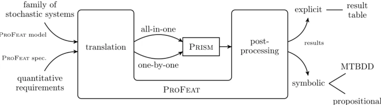
post-ProFeat family of stochastic systems quantitative requirements explicit symbolic result table MTBDD propositional formula ProFeatmodel ProFeatspec. all-in-one one-by-one results
Fig. 1. Workflow overview
Prism[KNP11], implementing the formal framework of [DBK15]. To specify valid feature combinations and to describe the structure of the family of systems, we rely on a feature-model formalism similar to the Textual Variability Language (TVL) [CBH11]. ProFeat also allows for (numerical) feature attributes and multi-features [CHE05, CBH11, CSHL13], i.e., multi-features that can appear more than once in a feature combination. Following [DBK15], the behaviors of each feature are specified infeature modules described by discrete- or continuous-time Markov chains or Markov decision processes. The support for dynamic feature switches dur-ing runtime is maintained by a module calledfeature controller, which synchronizes with the feature modules when activating and deactivating features. The dynamics of the feature controller and its interactions with the feature modules are crucial to model dynamic product lines [GH03, DMFM10, DS11, CCH+13a].
(2) ProFeat follows a translational approach towards a quantitative analysis of system families, il-lustrated in Figure 1. In a preprocessing step, ProFeatfamily models and quantitative requirements are translated into the pure input language ofPrism. Then, the actual analysis is performed by invokingPrism
on the translated models and requirements, returning results through Prism logs. The returned logs are post-processed and ProFeatrepresents the results for each family member in the feature-aware context. Note that using this approach, ProFeat can benefit from the power of the state-of-the-art probabilistic model checkerPrismand its (possibly future) extensions.(3)Since the number of family members can be exponential in the number of features, just providing enumerated results for each member can be cumber-some in the feature-aware engineering process. Thus,ProFeatprovides compact symbolic representations of the results using MTBDDs or propositional formulas over features.
We evaluate the approach of using ProFeat in a feature-oriented engineering process by several case studies.(4)ProFeatseamlessly integrates both one-by-one and all-in-one analysis without requiring adap-tions to the family model and specification (see (1)). This is obtained through different translation and post-processing mechanisms and fits into the feature-oriented analysis approach: When there are many com-monalities within family members, a symbolic model-checking engine might be chosen inPrismto exploit the commonalities within an all-in-one approach and speed up the analysis.(5)Since the symbolic MTBDD rep-resentation of the family is sensitive to the chosen variable order, we investigate the application of automated reordering techniques recently introduced inPrism[KBC+16].ProFeatfully supports the maintenance of
the variable reordering, such that no adaptions to the family model is required to enable or disable reordering techniques.
(6) Besides useful for the quantitative analysis of families of stochastic systems,ProFeat can also be used to describe single dynamic stochastic systems where features model operational modes of the system. Feature switches then model the dynamic mode switches during runtime of the system. To underpin this statement, we carry out a case study issuing the feature-oriented engineering process of an energy-aware adaptive network system.
The source code of ProFeat can be obtained at https://wwwtcs.inf.tu-dresden.de/ALGI/PUB/ ProFeat. This paper is an extension of the conference version [CDKB16], whereProFeathas been presented first. There, the symbolic representation of analysis results was not included inProFeatyet. Furthermore, the seamless integration of automated variable reordering techniques for symbolic analysis engines [KBC+16]
has been newly integrated. Additional case studies and more detail on the feature-oriented engineering ap-proach with ProFeat is provided. In contrast to our previous work [DBK15], where we introduced the
formal frameworkProFeatis relying on, theProFeatapproach provides an elegant way to specify feature modules and the feature controller and to automatically generate corresponding Prismcode, rather than requiring a handcrafted translation from formal descriptions of Markov decision processes toPrismas done in [DBK15].
Related work. Several techniques for the analysis of (non-probabilistic) feature-oriented models and soft-ware product lines using testing, type checking, static analysis, theorem proving or model checking have been already proposed and implemented in tools (see, e.g., [TAK+14] for an overview). Commonly, feature-aware
analysis techniques try to avoid the combinatorial blowup in the number of features arising when analyzing all members of a feature-oriented system family separately. Symbolic representations of the family and ap-propriate algorithms to reason about the whole family at once turned out to be very successful. ProFeat
complements most of the existing approaches by not tailoring feature-aware analysis algorithms but fully relying on standard model-checking tools and exploiting their symbolic representations of the systems. Here, we briefly summarize tool support for the analysis of feature-oriented systems using model checking. An overview about theoretical considerations towards these tools and prototype implementations in the litera-ture can be found in [DBK15], where the formal frameworkProFeatis based on has been developed. For the automatic detection of feature interactions, Plath and Ryan [PR01] introduced a feature-oriented extension of the input language of the model checker SMV and Apel et al. [ASW+11] presented the tool SPLVerifier.
FeatureIDE [TKB+14] is a tool set supporting all phases of the software-product-line development with
connections to the theorem prover KeY and the model checker JPF-BDD. Lauenroth et al. [LPT09] deal with family models based on I/O automata with may (“variable”) and must (“common”) transitions and a model checker for a CTL-like temporal logic that has been adapted for reasoning about the variability of product lines. Featured transition systems (FTS) are labeled transition systems with annotations for the feature combinations of static product lines [CCS+13] or a variant of dynamic product lines [CCH+13a].
The SNIP tool [CCH+12, CCS+13, CSHL13] relies on FTS specified using a feature-based extension of
the modeling language Promela and allows for checking FTS against LTL properties one-by-one or using a symbolic all-in-one verification algorithm. Its re-engineered version ProVeLines [CCH+13b] provides several
extensions, including verification techniques for reachability properties with real-time constraints. Similar to the approach by [DKB14] for probabilistic product lines, [DABW15] considers (non-probabilistic) product-line verification of product-linear-time requirements and presents an approach that avoids specialized feature-aware model-checking algorithms. For branching-time temporal-logic specifications, [CCH+13a, CCH+14] proposed
a symbolic model-checking approach for (adaptive) FTS. We are not aware of an implementation of the ap-proach of [CCH+13a]. Relying on the formal framework of [AtBGF11, tBFGM16], where product line families
are modeled through modal transition systems, the tool Vmc has been presented in [tBMS12] that allows for the verification of branching-time requirements.
In [CCH+14], an all-in-one analysis based on the feature-oriented extension of the SMV input language
by [PR01] has been proposed, which allows verifying static product lines using the (non-probabilistic) sym-bolic model checker NuSMV. This extension of SMV follows the compositional feature-oriented software design paradigm (as we do) but puts the emphasis on superimposition [Kat93, AJTK09, AH10], rather than parallel composition of feature behaviors [DBK15].
None of the approaches mentioned above deals with probabilistic behaviors. To the best of our knowl-edge, there is no other tool that provides family-based probabilistic model checking for families using a compositional framework based on Markov decision processes. An overview about quantitative analysis for probabilistic product lines can be found in [LP17]. The benefits of probabilistic model checking for the analysis of adaptive software has been also drawn by Filieri et al. [FGT12], where adaptive Markov chains models were investigated within a continuous verification approach. There, the focus was not on a family-based analysis but on a holistic approach towards supporting required adaptations to environmental changes. The work on model-checking algorithms for parametric Markov chains [Daw04, HHZ11] and tool support in the model checkers Param [HHWZ10] (which has been reimplemented and integrated in Prism) and
PROPhESY [DJJ+15] is orthogonal. By computing rational functions for the probabilities of reachability
conditions or expected accumulated costs, these techniques can be seen as an all-in-one analysis of fam-ilies of probabilistic systems with the same state space, but different transition probabilities. Ghezzi and Sharifloo [GS13] and the recent work by Rodrigues et al. [RAN+15] illustrate the potential of parametric
probabilistic model-checking techniques for the analysis of product lines.ProFeat can handle probability parameters as well and translate them toPrismcode, such that models used in [GS13, RAN+15] can also
different in the sense that the probability parameters are encoded as model variables, using the standard engines of Prismrather than its parametric one. An approach towards a family-based performance analysis of dynamic probabilistic product lines modeled by a variant of UML activity diagrams has been presented by [KST14]. Dynamic changes on the performance-annotated activity diagrams (PAADs) are expressed us-ing the delta-modelus-ing approach [Sch10], which complements the compositional approach by [DBK15]. Our approach covers the class of models considered, as the semantics of PAADs is given as a very restricted class of CTMCs. Thus, ProFeat could also be applied to analyze PAADs. However, since [KST14] uses specialized algorithms to avoid explicit encodings into the state space thatProFeatdoes not provide, only small instances are feasible to analyze withProFeat. The recent work by Beek et al. [tBLLV15] presents a framework for the analysis of software product lines using statistical model checking. They focus on Markov chain models rather than Markov decision processes and present a process-algebraic characterization of feature-oriented concepts.
Outline. Section 2 presents the main principles of theProFeatlanguage to describe families of stochastic systems. The standard feature-oriented engineering process withProFeatis described in Section 3. Details on the implementation of ProFeat will be given in Section 4. Section 5 reports on experimental studies withinProFeat. A brief conclusion is provided in Section 6.
2. Describing Families of Stochastic Systems: The
ProFeat
Language
TheProFeatlanguage can be seen as an extension of the input language of the probabilistic model checker
Prism[KNP11] that is used for modeling and analysis of parallel probabilistic systems. Prismand hence
ProFeatsupports various types of finite system models such as discrete- or continuous-time Markov chains (DTMCs, or CTMCs, respectively) and Markov decision processes (MDPs).
In this section, we present the additional language concepts introduced for the analysis of families of stochastic systems. In Section 2.1 we will first give a brief summary of the corePrismlanguage. Section 2.2 introduces the meta-programming language constructs as a first class of extensions provided by ProFeat. These meta-programming constructs, such as parameters, arrays, and loops facilitate the feature-based mod-eling of families of stochastic systems, but are useful in general as well. The main language concepts for the compositional description of system families (cf. [DBK15], Section 4) are introduced in Section 2.3.
In what follows, we describe the ProFeat language using a simple producer-consumer example. The system consists of a single producer that enqueues jobs with probabilistic workload sizes into a FIFO buffer handed to one or more workers. The workers can only process one package at a time each. The time it takes for a worker to process a work package is determined by the package size and the processing speed of the individual worker. Varying the buffer size, the number of workers, the processing speed of individual workers or the load caused by the producer yields different variants, i.e., families of systems.
2.1. The
Prism
Language
A model in the input language of Prism[KNP11] consists of one or more reactivemodules [AH99] that can interact with each other. A set of variables defines the local state space of a module and the local variables of all modules constitute the global state space of the model.Prismsupports two types of variables: bounded integers and Boolean variables. The behavior of a module, i.e., the possible transitions between its states, is given by a set ofguarded commands [Dij75]. A command has the form:
[action-name] guard→p1: update1 + p2: update2 +. . .+ pn: updaten
The guard is an expression over the variables of the model (including local variables of other modules). If the guard evaluates totrue, the module can transition into a successor state by updating its local variables. One of the updates is chosen according to the probability distribution given by expressionsp1, p2, . . . ,pn. In every state (fulfilling the guard) the evaluations of these expressions must sum up to 1. A command can be labeled with an action name. They stand foractions used for synchronization between modules. If two or more modules share an action, they are forced to take the labeled transitions simultaneously. However, if any of those modules cannot take the transition (because its guard is not fulfilled), then the action isblocked, so that none of the modules can take the transition. Listing 2 shows an example of a simple producer that
module Producer work_size : [1..2];
[enqueue] !buffer_full -> 0.7: (work_size’ = 1) + 0.3: (work_size’ = 2);
endmodule
Lst. 2. A module for a simple producer in thePrismlanguage
enqueues a work package into the buffer whenever the enqueueaction is not blocked and the buffer is not full. The work package size is determined probabilistically, where a bigger work package is produced with a probability of 0.3.
Constants can be defined using theconstkeyword. A constant definition has the formconsttype = ex-pression. Here, thetype is either bool,int or double. Additionally, the formulakeyword can be used to introduce a shorthand name for an expression to reduce code duplication. In contrast to constants, aformula may be defined in terms of model variables.
A model can be annotated with costs and rewards1 using reward structures in order to reason about quantitative properties, such as energy consumption, throughput and performance. Costs and rewards are real values attached to certain states or transitions of the model. A state reward definition has the form guard : reward, indicating that every state fulfilling the guard has the specified reward associated with it. Similarly, the definition of a transition reward is of the form[action-name] guard : reward. Here, all transitions originating from a state fulfilling the guard and labeled with the given action have the specified reward attached to it.
2.2. Metaprogramming Language Extensions
ProFeatprovides several extensions to thePrismlanguage that allow the user to parametrize parts of the system. This is especially important for modeling system families. Besides Boolean and integer variables,
ProFeatsupports (one dimensional) arrays. Additionally, theProFeatlanguage offers metaprogramming constructs commonly found in template languages.ProFeatallows the parametrization ofPrism’sformula definitions to define function-like macros. Furthermore, ProFeat supports for loops. Loops can be used to generate sequences of commands, probability distributions, variable updates and expressions. This is especially useful for the definition of system families where the instances differ in their structure, e.g., buffer sizes or the number of multi-feature instances. In the following example, a parametrized formula that stands for the expression summing up the firstnelements of an array is defined:
formula sum(arr, n) = for i in [0..n-1] { arr[i] + ... };
If a for loop is used in an expression (as is the case in the example above), the body of the loop must contain the placeholder...exactly once. Intuitively, in iteration stepithis placeholder is replaced with the resulting expression of the iteration stepi+ 1.
Prior to the translation of a ProFeat model into a Prism model, macros defined via the formula keyword are expanded at all call sites. Similarly, forloops are expanded generating ProFeat code. For example, the callsum(buffer, 4)of the macro defined above is expanded to:
buffer[0] + buffer[1] + buffer[2] + buffer[3]
InProFeat, actions can be used and indexed like arrays. The size of an action array does not need to be declared. Arrays of actions are useful in conjunction withforloops, for example:
for w in [0..2]
[dequeue[w]] cell != -1 -> (cell’ = -1);
endfor
1 In the following, we use the notions of costs and rewards synonymously. Conceptually they are the same, it is only the
System
Fast Producer Workers Buffer
Worker0 speed:[1..5] Worker1 speed:[1..5] Worker2 speed:[1..5]
Fig. 3. Feature diagram of the producer-consumer product line Here, three distinct actions are generated:dequeue[0],dequeue[1] anddequeue[2].
2.3. Feature-oriented Language Extensions
A ProFeat model usually comprises two distinct parts: the declaration of a family parameters and/or feature combinations, and a modular (feature-oriented) representation of the operational behavior for all building blocks of the family model. For the definition of the operational behaviors, we adopt the guarded-command input language ofPrismand extend it with the feature-specific concepts as presented in [DBK15]. First, the guards used in transition definitions within aPrismmodule can now contain constraints on the activity of the declared features. Second, to specify dynamic product lines in which features can be activated and deactivated “at runtime”, an additional Prism module called feature controller can be added that is responsible for performing the feature switches. The syntax for specifying the feature controller is the same as for otherPrismmodules, but allows for feature activation and deactivation in the update part of transition definitions. Additional action names that can be used for synchronization with other modules are inserted automatically when a feature controller is specified.
Feature Models inProFeat.ProFeatprovides additional support to describe families of systems that correspond to (software) product lines. Within product lines, the standard formalism to define feature models in the software-engineering domain is provided byfeature diagrams [KCH+90]. Figure 3 depicts the feature diagram for the producer-consumer example. Nodes in the diagram denote features and the root node stands for the so-called root feature. Arcs connect an inner node with its children, namely the sub-features of the respective feature. They can be of different type imposing certain constraints on the the set of valid feature combinations. In the example, the root featureSystemhas four sub-features. Three of them are mandatory in valid feature combinations, only theFastfeature is optional (indicated by the circle on the corresponding arc). The Workers feature has three sub-features for the workers. The arcs imply that at least one of the workers must be active in all valid feature combinations. Moreover, there can be arrows indicating additional dependencies possibly across the entire diagram. For instance, the arcs betweenFast and Worker0/Worker1
stand for the constraint that fast systems need to have at least two active workers. There are many other possible annotations to feature diagrams, e.g., feature attributes (as thespeedin Figure 3) and cardinalities indicating the minimum or maximum number of instances of the same feature that could be activated, etc. Feature diagrams are usually conveniently described using the Textual Variability Language (TVL) [CBH11] and we adapt the concepts of TVL for describing feature models also inProFeat. To provide an example, Listing 4 is an excerpt of the producer-consumer feature model. Features are declared within feature blocks indicated by the keywords featureand endfeature. The root featureis a designated feature that rep-resents the base functionality on which the product line is built. In the given example the root feature is theSystemfeature, which is decomposed into the four sub-features. Anall ofdecomposition indicates that all sub-features are required in every feature combination whenever their parent feature is active. As used by theWorkers feature, the some ofoperator implies that at least one of the sub-features has to be active whenever the parent is active. In addition to theone ofoperator (which requires exactly one sub-feature), the decomposition can also be given by a cardinality. Optional features are preceded by theoptional
key-1 root feature
2 all of Producer, Buffer, Workers, optional Fast;
3 constraint active(Fast) => active(Worker[0]) & active(Worker[1]); 4 constraint Worker[0].speed + Worker[1].speed < 7;
5 endfeature 6 7 feature Workers 8 some of Worker[3]; 9 endfeature 10 11 feature Worker 12 speed : [1..5]; 13 endfeature
Lst. 4. Excerpt of the feature model for the producer-consumer product line
word, indicating that the feature may or may not be part of a valid feature combination, regardless of the decomposition operator.ProFeatalso provides support formulti-features [CSHL13], i.e., features that can appear more than once in feature combinations. The number of instances is given in brackets behind the fea-ture name. In the producer-consumer example, theWorkersfeature is decomposed into three distinct copies of theWorker feature. It is important to note that the decomposition operator ranges over the feature in-stances. Thus, thesomeoperator could be replaced by cardinality[1..3]in the above listing. Multi-features can be marked optional as well. Then, each individual copy of the multi-feature is an optional feature. Besides multi-features, the ProFeatlanguage supportsfeature attributes [CBH11]. In the example shown above, theWorker features carry the attribute speedwhich can take any integer value from 1 to 5. Access to feature attributes, e.g., in guards of transition definitions within other features, is possible regardless of whether the corresponding feature is active or not. Multi-features and feature attributes in combination as supported by ProFeatallow for compact textual descriptions of large and rather complex product lines. The support for multi-features requires the distinction between features and feature instances. InProFeat, each feature instance has to be uniquely identified by afully qualified name. Sub-feature instances as well as feature attributes are accessible using the familiar dot-notation. Instances of multi-features are referred to by an array-like syntax. For example, the fully qualified name of the second worker’s speed attribute is root.Workers.Worker[1].speed. As long as the qualified name is unambiguous, the prefix can be omitted. For instance, the name Worker[1].speedis valid as well. Within the local scope of a feature one can refer to its attributes without a qualifier. For example, within the feature module of Worker (Listing 5, line 9), speedrefers to the local attribute of the feature.
As seen already in the feature diagram, features may also contain cross-tree constraints and dependencies on feature instances and values of feature attributes. In our example, the first constraint (line 3) given in
the root feature expresses that the first two Worker instances must be active whenever the Fast feature is active. The second constraint limits the accumulated speed of the first two workers. A constraint can be preceded by theinitialkeyword, which only affects the initial set of valid feature combinations. Obviously, this distinction is only relevant for dynamic product lines.
Operational Behavior of Features.In a ProFeatmodel, the declarative feature model is strictly sep-arated from the operational behavior of features. A feature can be “implemented” by one or more feature modules, which are listed after the modules keyword inside the featureblock. In the producer-consumer example, theWorkerfeature is implemented by theWorker_implmodule. Listing 5 shows the feature module and the extended feature declaration of theWorkerfeature.
For the definition of feature modules, we use an extension ofPrism’s modules (as described in Section 2.1). Local variables of other features can be accessed using the dot-notation as described above. Access to local variables of feature modules is possible regardless of whether the corresponding feature is part of the current feature combination or not. If a feature is deactivated, its state (i.e., the local variables) remains unchanged and can still be read. To the standard language constructs already present in Prism, ProFeat adds the predicateactivethat can be used in any expression including guards, evaluating totrueif the corresponding
1 feature Worker 2 speed : [1..5]; 3 block dequeue[id]; 4 modules Worker_impl; 5 endfeature 6 7 module Worker_impl 8 t : [0..max_work_size] init 0;
9 [working[id]] t > 0 -> (t’ = max(0, t - speed)); 10 [dequeue[id]] t = 0 -> (t’ = Buffer.cell[0]); 11 endmodule
Lst. 5. Declaration and implementation of theWorker feature 1 controller
2 [] buffer_full & !active(Worker[2]) -> activate(Worker[2]); 3 [] buffer_low & active(Worker[2]) -> deactivate(Worker[2]); 4 endcontroller
Lst. 6. The feature controller of the producer-consumer model
feature is active in the current system state. Furthermore, actions can either be declared as blocking or non-blocking. By default, feature modules of inactive features do not block on synchronous actions. Thus, with regard to synchronization, deactivating a feature has the same effect as removing it entirely from the model. This is useful if the model is fully synchronous, i.e., if there is a global action that synchronizes over all transitions. However, in some cases it is crucial that an inactive feature hinders active features to synchronize with its actions. In the producer-consumer example, an inactive worker should not take a work package out of the queue (line10in Listing 5). Therefore, its dequeueaction is modeled as blocking using theblock keyword inside the feature module (line 3). For thedequeue action, we use an indexed action label with theidas index. In case of multi-features, the implicitidparameter evaluates to the index of the feature instance.
Feature Controller.In aProFeatmodel, the feature combination is not necessarily static, but may also change over time. Thefeature controller is a special module that defines the rules for the dynamic activation and deactivation of features. In Listing 6, one can see an example of a feature controller suited for the producer-consumer model.
Essentially, acontrolleris a module (possibly with its own internal memory), which can modify feature combinations using theactivateanddeactivateupdates. In the controller shown above, the third worker is activated to speed up processing whenever the buffer is full. Once the buffer is nearly empty, the worker is deactivated. The definition of a feature controller is optional. If no controller is given, the defined product line is assumed to be static. Feature modules can synchronize with the controller over the activate and deactivate actions, which enables them to react or even block the activation or deactivation of their corresponding feature. For instance, by adding the following line to theWorker_implmodule, the deactivation of the worker is blocked as long as it is still processing a work package:
[deactivate] t = 0 -> true;
Feature Templates and Module Templates. Both featureblocks as well as feature modules can be instantiated multiple times. Every time afeatureis referenced in a decomposition, a new instance of that feature is created. Additionally, all of its associated feature modules are instantiated as well. Thus, both featureblocks and feature modules can be regarded as reusable templates. Furthermore,ProFeatallows the parametrization of these templates, which in turn enables parametrization of guards, probabilities and costs.
1 feature Buffer
2 modules fifo(buffer_size); 3 endfeature
4
5 module fifo(capacity)
6 cell : array [0..capacity - 1] of [-1..max_work_size] init -1; 7 for w in [0..2]
8 [dequeue[w]] cell[0] != -1 -> 9 (cell[capacity-1]’=-1) &
10 for i in [0..capacity-2] (cell[i]’ = cell[i+1]) endfor; 11 endfor
12 . . .
13 endmodule
Lst. 7. A FIFO buffer implementation parameterized over the capacity 1 const double dist = binom(0.3, max_work_size-1);
2
3 module Producer_impl
4 work_size : [1..max_work_size] init 1; 5 [enqueue] true ->
6 for i in [1..max_work_size] 7 dist[i-1]: (work_size’=i) 8 endfor;
9 endmodule
Lst. 8. A producer implementation with parameterized probability distribution over the work package size Consider the Buffer feature and its accompanying feature module shown in Listing 7. The module is parameterized over the capacity of the buffer (line 5). The actual buffer size will be determined on
instantiation. In the given example, the buffer size will even be declared as system parameter ranging over a finite set of possible values. Theforloop stretching from line7to 11 generates adequeuelabeled command for each worker. The inner loop (line10) shifts the buffer entries to remove the first element from the buffer. The feature module of theProducerfeature (Listing 8) is parameterized over the maximal size of a work package. Because of that, the support of the probability distribution over the size of the next work package is not fixed (lines5–7). For cases like that,ProFeatcan generate probability distributions of a given size.
In the example, the work package size is binomially distributed (line1and line7). Currently,ProFeatonly
supports binomial distributions, however, other discrete distributions may be added in the future.
2.4. Parametrization
Families can also be formed by ranging over system parameters. In our running example, such a parameter might be the FIFO buffer size. System parameters are declared in afamilyblock, as shown below. Similar to feature attributes, system parameters can be constrained as well.
Furthermore, a family declaration can be combined with a feature model, resulting in a family that is both defined by system parameters and all valid initial feature combinations. This is of particular importance for dynamic product lines where there is an initial feature combination that can evolve over time. To declare subsets of valid feature combinations as initial ones,ProFeatprovides theinitial constraint keyword (see line3of Listing 9). Valid feature combinations not fulfilling the listed constraints are still possible during
runtime by dynamic feature switches.
1 family
2 buffer_size : [1..8];
3 initial constraint buffer_size != 5; 4 endfamily
Lst. 9. Parametrization of a model using thefamilyblock
1 feature Worker 2 rewards "energy"
3 active(this) & t > 0 : 1; 4 [activate] true : 5; 5 endrewards
6 endfeature
Lst. 10. Specification of the energy consumption of aWorker
costs/rewards. In contrast to feature attributes, system parameters are constant for each instance of a family. By an instance of a family we mean a particular system or product in the product line. This has an important consequence: parameters can, e.g., be used to specify the range of variables, the size of arrays, the range of forloops and even the number of multi-feature instances. Thus, system parameters can directly influence the state space of the system.
2.5. Property Specification in
ProFeat
ProFeatuses an extension of Prism’s property specification language, which is based on the probabilistic computation tree logic (PCTL) [BdA95, BK98]. Reasoning about probabilities in an MDP requires the selection of an initial state and resolution of the non-deterministic choices between actions. The latter is formalized by a scheduler. In the following, we write Prmin(ϕ) for the minimal probability of that ϕ is fulfilled, ranging over all schedulers. For the specification of path properties, we use the usual temporal operatorsG(globally) andF(finally). We consider two example properties of the producer-consumer model. The following property states that the filling level of the buffer is almost surely below 75%, even in the worst case:
Prmin G(level<0.75)
= 1
One can also ask for computing, e.g., the minimal probability that at some pointWorker2 is active, which
could be expressed by
Prmin F(“Worker3 is active”)
As in the Prismlanguage, a ProFeat model can be annotated with costs and rewards. However, reward structures are not global, instead they are defined within feature declarations. This modularizes the speci-fication of rewards and furthermore enables the parametrization of rewards inside of parametrized feature declarations. ProFeatextends the reward construct of Prismby allowing the use of the activefunction to specify rewards in terms of the current feature combination. Additionally, rewards can be attached to feature switches by using the predefinedactivateanddeactivate actions. This enables quantitative rea-soning about dynamic software product lines. Listing 10 shows again the declaration of theWorker feature and its reward structure. In line 3, energy costs of 1 are specified for all states where theWorker is active and not idle. The activation of the feature (line 4) has a cost of 5.
The second property specifies that even in the worst case, the maximal expected energy consumption of the producer-consumer system does not exceed a given threshold. Here,goaldenotes the state where all
1 formula level = (for i in [0..buffer_size-1]
2 (cell[i] > 0 ? 1 : 0) + ...
3 endfor) / buffer_size; 4 Pmin>=1 [ G (level < 0.75) ];
5 Pmin=? [ F (active(Worker[2])) ]; 6
7 const threshold = 20;
8 label "goal" = (counter = 0) &
9 for w in [0..2]
10 (active(Worker[w])) => Worker[w].t = 0 & ... 11 endfor;
12
13 R{"energy"}max<=threshold [ F "goal" ];
Lst. 11. Property specifications using the language extensions of ProFeat
work packages have been processed and each activeWorkeris idle.
Exmax(“accumulated energy until reachinggoal”)≤threshold
Listing 11 shows the properties in the specification language of ProFeat. In the definition of the atomic propositiongoal(lines 8–11) we use aforloop to iterate over allWorkerinstances. Theactivefunction can be used in the same way as in aProFeatmodel as well as the access of qualified variables (such as the t variable of aWorkerin line 10).
2.6. Semantics of
ProFeat
Models
As in thePrisminput language, every model inProFeathas to begin with identifying the kind of model specified, i.e., either a discrete Markov chain (DTMC, keyworddtmc), continuous-time Markov chain (CTMC, keyword ctmc), or Markov decision process (MDP, keyword mdp). The semantics of the ProFeat model then is then a family of formal models of DTMCs, CTMCs or MDPs, respectively. We depart from explicitly providing a formal semantics for ProFeat models since it can be obtained in a straight-forward way by the following three ingredients: First, ProFeatfully relies on the framework of [DBK15], where a formal semantics for feature modules and feature controllers has been provided. Second, the semantics ofProFeat’s feature modeling formalism is given by the semantics of TVL [CBH11] extended with multi-features as described in [CSHL13]. Third and last,ProFeatuses a translational approach towardsPrismmodels, which have a formally defined semantics [KNP11]. We refer to Section 4, where the details on the implementation of howProFeatmodels are translated to purePrismmodels are provided.
3. Family-based Analysis with
ProFeat
In this section, we describe the general workflow for analyzing families of systems specified in theProFeat
language using our implementation2. As depicted in Figure 1, the ProFeatapproach comprises a prepro-cessing, analysis, and post-processing step for the analysis of families of stochastic systems. The standard of the ProFeat approach is that all three steps are executed in a row. However, the designer can also decide to perform these steps separately, which is useful, e.g., when the translated model(s) should further be processed, be simulated within the Prismsimulator for debugging, or analyzed using some alternative tool or different analysis engine.
Let us now consider the standard case where the family-based analysis usingProFeatis performed in one run. First, the designer decides which analysis engine provided byPrismwill be used for the analysis. This
decision mainly depends on how the members of the family of stochastic systems share common behaviors. In case there are lots of commonalities, e.g., when the main functionalities are encapsulated into one feature module included in all family members, a symbolic engine is usually the best choice. Also if the model of each family member is as huge that it would possibly not fit into the memory, an analysis still might be successful when using a symbolic engine. In this spirit, also the decision whether an all-in-one or one-by-one analysis is used by ProFeat is made: when a symbolic engine is chosen, commonalities in the members of the described family can be further exploited by choosing an all-in-one analysis approach. Within an all-in-one analysis,ProFeatgenerates a singlePrismmodel of the whole family which could be compactly represented within a symbolic representation of the family model. As the symbolic engine of Prismrelies onmulti-terminal binary decision diagrams (MTBDDs), the performance and memory consumption of the analysis crucially depends on the variable order inside the MTBDD. The designer has the choice of using automated reordering techniques [KBC+16], which could provide a further speed up of the analysis. On
the other hand, when an explicit analysis engine is chosen, one-by-one approaches are usually favorable. In this case,ProFeatgenerates onePrismmodel for each family member, not exploiting commonalities but enabling the parallelization of the analysis, e.g., using multiple cores or distributed computation.
After the decisions about the analysis methods are made, the designer chooses how the analysis results should be represented.ProFeatsupports both, explicit and symbolic representations of the analysis results for each family member. For families described by only a few features, an explicit representation of the results in terms of a table is usually sufficient. However, when the family described involves many features, the number of family members and thus the number of analysis results can be exponential in the number of features. This makes an explicit representation of the results difficult to interpret by the designer during the feature-oriented engineering process. To avoid the combinatorial blowup in the result representation,
ProFeat provides symbolic representation of the results. The designer can choose between propositional formulas or representations based on binary decision diagrams (BDDs) for describing the solution space.
In the following, we provide details on theProFeatapproach by first describing the concept of symbolic representations using BDDs. Then, we illustrate the pre- and post-processing steps using the simpleProFeat
model provided in Listing 12 as an example. The model comprises the declaration of the feature model (lines 1-8) and the implementation of the base feature and the two feature modulesxand y(line 10-23). In this example, no feature controller is provided, i.e., the resulting family is assumed to be static. Each feature module implementation has a local statestate. Access to the local state of a feature module implementation is performed by qualifying the scope of the state variable, e.g.,x.stateto refer to the local of the featurex.
3.1. Symbolic Representation by Binary Decision Diagrams
Binary decision diagrams (BDDs) have first been introduced by Lee [Lee59] and Akers [Ake78] as universal data structure for Boolean functions. In the context of model checking, BDDs are, e.g., used to represent the characteristic function of the transition relation for state-based models.
A BDD induces a rooted, directed, and acyclic graph comprising terminal nodes (representing the constant functions zero and one) and decision nodes. Each decision node is labeled by a Boolean variable and has exactly two successor nodes, where for the0-successor node, the respective Boolean variable is assigned to
falseand the for the1-successor node totrue. Figure 18a shows a simple example of a BDD graph structure, where the 0-successors are indicated by a dashes lines and the 1-successor by solid lines. Ordered BDDs
[Bry86] rely on a fixed variable ordering that it used consistently along all paths from the root to a sink. The graph structure of an ordered BDD for a Boolean function f arises from a binary decision tree forf using the given variable ordering by merging isomorphic subgraphs and eliminating terminal nodes with the same value and any node whose two children are isomorphic. This yields a reduced ordered BDDs (briefly called BDD from now on), where every two BDD nodes represent different functions. Removing redundancies from the decision tree and hence the sharing of structure in BDDs yields the potential of compactly representing Boolean functions. When using BDDs to represent family models, this means that ideally behavior that is common amongst all family members as, e.g., a base feature included in every family member, has to be represented only once.
In general, the size of an BDD, namely the overall number of BDD nodes, crucially depends on the given variable ordering. There are Boolean functions that have a very compact BDD-representation independent from the chosen order. For instance, for the n-bit parity function the number of nodes is linear in n. For some Boolean functions, however, the size of the BDD varies from linear to exponential depending on the
1 root feature
2 all of optional x, optional y; 3 constraint active(x) => active(y); 4 modules base_impl;
5 endfeature
6
7 feature x modules x_impl; endfeature
8 feature y modules y_impl; endfeature
9
10 module base_impl
11 state : [0..1] init 0;
12 [tick] !(x.state = 1) & !(y.state = 1) -> 1/3:(state’=0) + 2/3:(state’=1); 13 endmodule
14
15 module x_impl
16 state : [0..1] init 0;
17 [] state = 0 -> 1/2:(state’=0) + 1/2:(state’=1); 18 endmodule
19
20 module y_impl
21 state : [0..1] init 0;
22 [tick] !(x.state = 1) -> 1/4:(state’=0) + 3/4:(state’=1); 23 endmodule
Lst. 12. Simple product line example inProFeat
given variable ordering. An example is the Boolean function for the most significant bit of the addition. Finally, there are Boolean functions for which no compact BDD-representation exists, e.g., the n−1-st bit
of the multiplication function. See, e.g, [Weg00] for further details on BDDs. Reordering algorithms such as sifting [Rud93, PS95], can be applied to dynamically improve the size BDD for a given Boolean function.
Multi-terminal binary decision diagrams [CFM+93] (MTBDDs), also known as algebraic decision
dia-grams (ADDs) [BFG+97], are a variant of BDDs that support terminal nodes with real values rather than
only0and1. MTBDDs are, e.g., used as data structure for representing and analyzing probabilistic systems.
The symbolic engine of Prism for instance, relies on MTBDDs for representing the transition probability matrix of the stochastic models. InProFeatwe use MTBDDs also to encode the computed results for all family members symbolically. Here, the decision nodes correspond to feature activation or deactivation and the terminals represent the model checking results such as probabilities and expectations.
3.2. All-in-one vs. One-by-one
In the example in Listing 12, the feature model describes a family comprising three feature combinations: the base feature alone, with theyfeature activated in addition to the base feature and all features activated. The combination thatxis solely activated besides the base feature is excluded through the constraint provided in line 3. When a one-by-one approach is chosen, ProFeatgenerates three different models, one for each feature combination and invokesPrismthree times (once for each generated model). Within the all-in-one approach,ProFeatgenerates one single model with three initial states.
Note that when the automated variable reordering techniques are used, each verification run may yield a different variable order. Thus, whereas in the all-in-one approach the family is represented by an MTBDD only with respect to one particular variable order, the variable orders between the models for a one-by-one analysis may differ.
Conceptually, it is possible to combine the all-in-one approach and the one-by-one approach. First, the set of instances of the system family is partitioned. Then, each element of the partition can be regarded as a sub-family, which is analyzed using the all-in-one approach. The partition can be determined by the user
Final result: [0.0,0.9876543209876543] Results for initial configurations:
(x, y)=0.0 (y)=0.73 ()=0.99
Lst. 13. Output of analyzing the simple product line withProFeat
and allows a trade-off between analysis time, memory usage, and the ability to parallelize the analysis. Von Rhein [vR16] reported that indeed the combined approach uses less memory than the all-in-one approach and less time than the one-by-one approach for selected (non-probabilistic) models.ProFeatprovides limited support for the combined approach. Within the family block, a set of feature instances can be selected. Features selected in thefamilyblock then only vary between the sub-families, while the other features vary within each sub-family. For an example, we consider again the producer-consumer model.
family
features Fast, Worker[2];
endfamily
If we add thefamilyblock given above, we get a partition consisting of 4 elements because two features are selected using thefeatureskeyword.
3.3. Post-processing: Output of the Analysis Results
ProFeat generates an output of the results similar to Prism, but for readability’s sake, listing only the valid feature combinations. If the analysis is carried out using the one-by-one approach where Prism is invoked for each instance of the family, ProFeat automatically collects the results. In case automatic variable reordering [KBC+16] was used during the analysis, ProFeatalso converts the variable ordering
of the results to a common ordering. Thus, the representation of the final results is independent of the chosen analysis approach. An example result generated byProFeatfor the example in Listing 12 is given in Listing 13. Here, we asked for the minimal probability such thatstate=1is reached in the base feature (formally, asking forPrmin(F(state= 1))).ProFeatsupportsrounding of the results up to a given precision and we chose a precision of two digits in our example. Rounding is very handy, e.g., if the results are close together and one likes to investigate the features with the most impact on the result. Currently,ProFeat
supports post-processing of analysis results only if the results were produced byPrism.
The representation shown in Listing 13 lists the results for each initial configuration separately. This is acceptable if just a small number of configurations is of interest. However, since the number of initial feature combinations is usually exponential in the number of features, it is difficult to draw general conclusions about the whole family of systems from this explicit representation of results. In order to give the user a better understanding of the analysis results,ProFeatcan additionally provide asymbolic result representations. Similarly to the analysis, where the symbolic representation of the model is often more compact than the explicit representation, a symbolic representation of the results is often smaller than the list of feature combinations.ProFeatcan compute two different symbolic representations. First,ProFeatcan generate a propositional formulaover features representing the feature combinations satisfying some qualitative property (similar to [CHS+10, CCH+13b]). This also includes quantitative properties where a certain threshold must
be reached. For example, asking for the feature combinations where (in the worst case)state=1is reached with a probability of at least 0.99 (formallyPrmin(F(state= 1))≥0.99), yields the result¬x∧ ¬y. Second,
ProFeat can produce a BDD, where each inner node stands for the decision whether the corresponding feature is included or not, and the terminal nodes indicate whether the property is satisfied or not. However, in case of a quantitative analysis, the result for a given feature combination is not just true or false, but can be any rational number. Therefore,ProFeatadditionally supports the symbolic representation of the results as an MTBDD. Here, each terminal node represents a distinct numerical analysis result. The rounding of the results can reduce the number of distinct results and, in turn, the number of terminal nodes as well as the overall size of the MTBDD. The BDD or MTBDD graph can be exported into the DOT-language
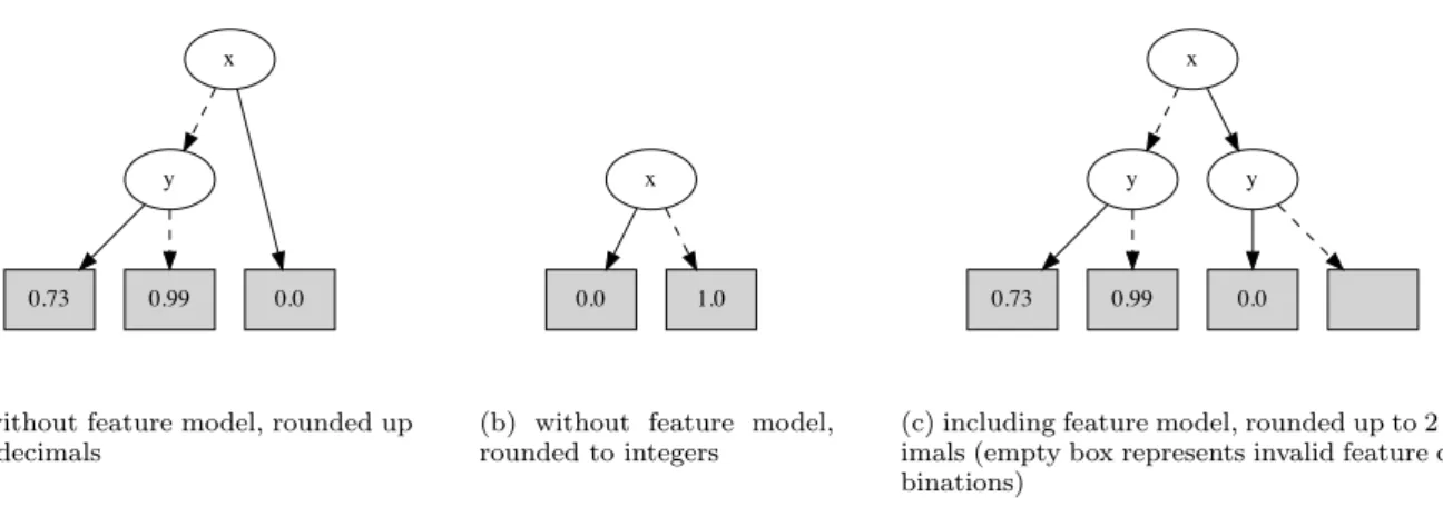
(that can then be rendered into graphs using Graphviz ). Details on how MTBDDs are used for yielding a user-friendly view on the results are presented in the next section. Examples of different outputs possible withinProFeatfor the analysis of the simple product line of Listing 12 are provided in Figure 18.
4. Implementation Details
In this section, we provide further details on our implementation of ProFeat. Feature model declarations follow the semantics of TVL [CBH11]. Based on the feature model, the translation of a set of feature modules under a feature controller into a Prismmodel is based on the compositional modeling framework for probabilistic feature-oriented systems presented in [DBK15], which naturally maps feature composition to the parallel composition ofPrism. The translation ofProFeatspecifications intoPrismspecifications is purely syntactical replacingProFeatlanguage identifiers by their translated correspondents in the generated
Prismcode.
In the following, we highlight the implementation of notable steps in the translation of ProFeatmodels intoPrismmodels, underpinned by examples from our running example of Section 2, the producer-consumer product line example. Furthermore, we describe different analysis methodologies supported byProFeatand give an overview on ProFeat’s result post-processing mechanisms. As illustrated in Figure 1, ProFeat
takes a ProFeatmodel, a ProFeat formula specification, and the choice of an analysis method (all-in-one or (all-in-one-by-(all-in-one) as input. The pre-processor translates the given model into a single Prismmodel or a collection of Prismmodels respectively. Additionally, the formulas given in theProFeatspecification file are translated into a standardPrismproperties file. This purely syntactical translation is necessary because the formulas of theProFeatspecification may contain language constructs not understood byPrism. These include, for example, qualified names for local variables and the built-in activefunction, which is used to refer to the current feature combination. After the translation step, ProFeat can automatically invoke
Prism and the results are being post-processed and presented such that they are readable in the feature context.
4.1. Translation of Feature-specific Constructs
In aProFeatmodel, read and write accesses to the feature combination are only possible by the use of the activefunction and theactivate/deactivateupdates, respectively. The basic idea is to add one Boolean variable per feature to thePrismmodel, indicating whether some feature is part of the feature combination. However, because features can be mandatory (must always be included in a feature combination) or can depend on each other, it is sufficient to generate one variable per non-mandatoryatomic set. An atomic set is a set of features that can be treated as a unit as they always appear together in a feature combination [Seg08]. For example, in case of the producer-consumer system family (Figure 3), the tool generates a feature variable for theFastfeature and one variable for eachWorker. Instead of Boolean feature variables,ProFeatgenerates integer variables with a range of[0..1], which simplifies the handling of cardinality constraints. Given this representation, the translation of theactivefunction is simple. If the atomic set of the feature is mandatory, the call is replaced by true. Otherwise, it is replaced by a check of the feature variable. Analogously, the activateanddeactivateupdates assign 0 or 1 to the corresponding variable, respectively.
Feature modules are translated to standardPrismmodules. In case of a feature module that implements a multi-feature, one module per feature instance is generated (with the id parameter set accordingly). Listing 14 shows the feature module of theWorker feature and its translation. Note that only the module corresponding to the firstWorkerfeature is shown, as the other instances are nearly identical. In the translated module, all local variables are qualified with their corresponding feature name as the Prismlanguage does not support local scopes. Additionally, the guard of each command is extended by the Worker_0_active predicate, such that the module has no behavior if the feature is inactive. However, it must be ensured that feature modules of inactive features do not block actions, i.e., deactivating a feature should have the same effect as removing the corresponding feature modules from the model. This is achieved by adding an unconditional transition for each non-blocking action. Such a transition can only be taken if the feature is
1 module Worker_impl 2 t : [0..max_work_size] init 0; 3 4 [] t > 0 -> 5 (t’ = max(0, t - speed)); 6 [dequeue[id]] t = 0 -> 7 (t’ = Buffer.cell[0]); 8 [cancel] true -> (t’ = 0); 9 10 endmodule
(a) Worker inProFeatmodel
module Worker_0_worker_impl
Worker_0_t : [0..max_work_size]; [] Worker_0_active & Worker_0_t > 0 ->
(Worker_0_t’ = max(0,Worker_0_t - speed)); [dequeue_0] Worker_0_active & Worker_0_t = 0 ->
(Worker_0_t’ = Buffer_cell_0);
[cancel] Worker_0_active -> (Worker_0_t’ = 0); [cancel] !Worker_0_active -> true;
endmodule
(b) Worker 0 inPrismmodel Lst. 14. Feature module of a worker and its translation 1 controller
2 [] buffer_full & !active(Worker[1]) -> activate(Worker[1]); 3 [] buffer_full & !active(Worker[2]) -> activate(Worker[2]); 4 [] buffer_low -> deactivate(Worker[2]);
5 [] buffer_empty -> deactivate(Worker[1]) & deactivate(Worker[2]); 6 endcontroller
Lst. 15. Feature controller for the producer-consumer model
inactive (see line 9 in Listing 14b). This command is not generated if the user explicitly requests the blocking of an action by using theblockkeyword in the feature declaration.
The feature controller is translated into a Prism module as well. Updates of the feature combination must not to lead to an invalid feature combination. Consider the update at line 4 of the feature controller in Listing 15. According to the feature model, at least one of theWorkers must be active at all times. Thus, the update is only allowed if there is at least one other active Worker. If not, this command should block. The described semantics is achieved by extending the guard in the translated module, as shown in Listing 16 (line 2). This guard is synthesized as follows. First, all constraints regarding the features to update (onlyWorker2 in this example) are collected from the feature model. Then, all feature variables that would be changed by the update are substituted with their updated value. Here, the variableWorker_2is replaced by 0, because the update would deactivate this feature. The resulting expression only evaluates to true if the updated feature combination is valid. Thus, an update command cannot lead to an invalid feature combination.
Another aspect of the translation concerns the synchronization between the feature controller and the feature modules in case of feature activation and deactivation. Consider again the feature controller shown in Listing 15. The command in line 4 implicitly synchronizes with the feature module in Listing 17a. To implement this synchronization, ProFeat generates action labels for feature activation and deactivation, as shown in line 1 of Listing 16. The command in line 5 of Listing 15 deactivates twoWorker instances at once, thus it also has to synchronize with both corresponding feature modules. However, in thePrisminput language each command can only be labeled with at most one action label. To circumvent this restriction, the set of action labels is merged into a single action label. This solution requires special care in the translation of the feature modules. First, we collect the action labels of all feature-controller commands that deacti-vate Worker 2 (lines 4 and 5). Then, we create a copy of the feature-module command for each collected
1 [Worker_2_deactivate] buffer_low &
2 (1 <= Worker_0 + Worker_1 + 0) & (Worker_0 + Worker_1 + 0 <= 3) -> 3 (Worker_2’ = 0);
1 module Worker_impl 2 t : [0..max_work_size] init 0; 3 4 [deactivate] t = 0 -> true; 5 6 7 8 endmodule
(a) Worker inProFeatmodel
module Worker_2_Worker_impl Worker_2_t : [0..2];
[Worker_1_deactivate_Worker_2_deactivate] Worker_2_active & Worker_2_t = 0 -> true; [Worker_2_deactivate]
Worker_2_active & Worker_2_t = 0 -> true;
endmodule
(b) Worker 2 inPrismmodel
Lst. 17. Translation of synchronization with the feature controller
action label, as shown in Listing 17b. This translation realizes the intended synchronization between the feature controller and the feature modules, even in the case of multiple simultaneous feature activations and deactivations.
4.2. All-in-One and One-by-One Translation
In case of a one-by-one translation, a model for each initial valuation of the system parameters and for each initial feature combination is created. The system parameters are constant for each instance and can therefore be replaced by constants in the translated models. However, the feature variables are not replaced by constants, as the feature combination may be changed by the feature controller.
For the all-in-one translation, ProFeat generates a single Prism model with multiple initial states, one for each instance of the family. However, there is a technical difficulty in the translation into an all-in-one model: Array sizes, numbers of multi-features and variable bounds can be defined in terms of system parameters. Hence, these system parameters depend on the initial state and thus are not known at translation time. In the producer-consumer model for example, both the buffer size as well as the number of workers may be defined in terms of system parameters. Since all family instances must be contained in the all-in-one model, ProFeat instantiates arrays with their maximal possible size, generates the maximal number of multi-feature instances and creates variables with the greatest possible bounds. These upper bounds can be computed from the range of the system parameters, which is known at translation time. In the example, thebuffer_size system parameter may range from 1 to 5. Then,ProFeat instantiates thefifo module (Listing 7) with size 5 in the all-in-one model. The need for instantiating all structures with their maximal size is the main reason that the all-in-one model is often substantially larger than (most of) the models generated by a one-by-one translation.
4.3. Post-processing of Analysis Results
As a consequence of the translational approach of ProFeat, the results of a quantitative analysis are ultimately produced by the used analysis tool. In the default case, this tool is Prism, which is the only analysis tool currently supported for the post-processing step byProFeat. Therefore, the analysis results actually refer to the translated Prismmodel rather than the ProFeat model. This means that variable names will not appear as written in theProFeatmodel. Furthermore,Prismhas no concept of features, thus feature variables are not easily distinguishable from other variables. However, the main issue is that the results as produced byPrismare hard to read, which makes their interpretation challenging.
As a first step, ProFeat rewrites variable names and feature names such that they appear as in the original ProFeat model and rounds the results up to a given precision. If the model investigated does not contain a feature model, i.e., the family described arises from parametrization only, ProFeatreturns the resulting list of results. We already presented an example output in Listing 13. Within each line the active features are now indicated with their names as provided in theProFeatmodel which increases the readability of the results.
Symbolic Representation of Feature-oriented Analysis Results.ProFeatrelies on standard model checking tools for the analysis. Therefore, the symbolic representations of the results are not directly provided
x
y
0.0
0.73 0.99
(a) without feature model, rounded up to 2 decimals
x
0.0 1.0
(b) without feature model, rounded to integers
x
y y
0.73 0.99 0.0
(c) including feature model, rounded up to 2 dec-imals (empty box represents invalid feature com-binations)
Fig. 18. Example MTBDD result representations withinProFeat
by the model checking algorithm. Thus, the propositional formula or the binary decision diagram representing the satisfying feature combinations must be computed from the list of results provided byPrism.
To generate a propositional formula representing the feature combinations satisfying some property, Pro-Feat proceeds as follows. The set of satisfying feature combinations directly corresponds to a formula in canonical disjunctive normal form, where the literals are features. Of course, this CDNF is as big as the explicit representation. In order to minimize this formula, ProFeat applies the Quine-McCluskey algo-rithm [McC56]4. As a consequence of this approach, the computed formula also encodes the feature model, or at least a part thereof. Since the feature model is already known before the analysis, one is usually more interested in the constraints that must hold inaddition to the feature model, such that the given property is satisfied. Formally, given a propositional formula Φencoding the feature model, we want to compute an
additional constraintΨ, such that all feature combinations of the (more restrictive) feature modelΦ0 = Φ∧Ψ satisfy the given property. To compute the constraint Ψ, we apply the Quine-McCluskey algorithm to the
set of satisfying feature combinations as described above, but also consider all invalid feature combinations as “don’t care” terms, which gives the algorithm more opportunities for minimization.
The BDD or MTBDD representation of the results is built by successively considering the result for each feature combination and adding the corresponding path to the MTBDD. ProFeatsupports two different modes to represent the MTBDD: including the feature model and not including the feature model. Because including the feature model often leads to a substantially larger and more cluttered MTBDD, the latter mode is the default. This representation can then be considered in addition to the feature model to guide the feature selection.
The MTBDDs in Figure 18a+b show the default representation without the feature model. The variables in the MTBDD correspond to the feature variables, evaluating to true if the respective feature is activated and to false otherwise. Solid lines indicate that the respective feature is active, whereas dashed lines indicate that the feature is deactivated. The sink nodes of the MTBDD carry all the possible values w.r.t. the considered analysis query. A path from the unique root node of the MTBDD to a sink node stands for the set of valid feature combinations that share a common result. Whereas in Figure 18a, the results are rounded to a precision of two digits, Figure 18b shows the same result rounded to integers, i.e., rounding probabilities to either 0 or 1. For the representation including the feature model, a sinkinv is included in the MTBDD
to which all paths of invalid feature combinations lead to. Figure 18c shows the MTBDD representation output including the feature model, where the empty sink corresponds to inv. This MTBDD degenerates into a binary tree, as all feature combinations have different values and there is exactly one invalid feature combination (in which only featurexis active).
4 The time complexity of this algorithm is exponential. Since the algorithm solves an NP-hard problem, no algorithm of
polynomial complexity can be expected. The families of systems suitable for quantitative analysis using model checking usually have a comparably small number of features. Thus, we have not encountered a model where the runtime of the Quine-McCluskey algorithm was the limiting factor.