Interatomic Potential Models
Seunghwa Ryu1 and Wei Cai2
1Department of Physics, Stanford University, California 94305
2Department of Mechanical Engineering, Stanford University, California 94305 E-mail: 1[email protected], 2[email protected]
Abstract. We report melting points and other thermal properties of several semiconducting and metallic elements as they are modelled by different empirical interatomic potential models, including Stillinger-Weber (SW), embedded-atom-method (EAM), Finnis-Sinclair (FS) and modified-embedded-atom-embedded-atom-method (MEAM). The state-of-the-art free energy methods are used to determine the melting points of these models within a very small error bar, so that they can be cross-compared with each other. The comparison reveals several systematic trends among elements with the same crystal structure. It identifies areas that require caution in the applications of these models and suggests directions for their future improvements.
PACS numbers: 64.70.D-, 65.20.-w, 65.40.-b, 02.70.Ns
1. Introduction
Empirical or semi-empirical potential models play an important role in computational materials science because many interesting processes involve the collective dynamics of thousands of atoms, which is still too expensive for ab initio models. At the same time, due to their (semi-) empirical nature, the potential models need to be thoroughly benchmarked before they can be trusted to make reliable, new, predictions. The structural and mechanical properties of a single phase (liquid or solid) have been extensively studied by computer simulations based on empirical potentials with considerable success. There is a growing interest in applying these models to study more complex processes, such as the catalytic growth of silicon nanowire from a eutectic liquid droplet, which involve the transformation between different phases. For these applications, it is very important for the potential models to provide a reasonable description of the melting point and other thermal properties. But the empirical potential models have not been extensively tested for these properties, mostly due to the difficulty in accurately determining the melting point.
Generally speaking, there are two ways to compute the melting point of a crystal from atomistic simulation. In the “co-existence method”, the liquid and solid co-exist with an interface in the simulation cell. The melting temperature is determined by finding the temperature at which both the liquid and solid phases are stable. While this method is easy to set up, fluctuations in the instantaneous temperature and the slow kinetics of solid-liquid interface motion introduce statistical and systematic errors in the estimation of the melting point [1, 2]. In the “free-energy” method, the Gibbs free energies of the solid and liquid phases are computed as functions of temperature, and the melting point is determined by their intersection point. The free energy method has been applied to determine the melting point of Stillinger-Weber(SW) model of silicon as early as 1987 [3]. Since then, several advanced free energy methods have been developed which make free energy and melting point calculations more efficient [4, 5], and many of them have been applied in melting point calculations [6]. While the free energy method is more difficult to set up, we find that it is more efficient than the interface method if we need to determine the melting point within a very small error bar, e.g.
±1K. The difficulty in setting up the various free energy calculations necessary for the determination of melting points is removed by the development of an automatic computer script [7].
In this paper, we show that accurate melting points can be obtained from the state-of-the-art free-energy methods. For the first time, we present a systematic comparison of the melting points, latent heat, entropy and thermal expansion coefficients of nine representative elements described by four different potential models, including Stillinger-Weber (SW) [8, 9], embedded-atom-method (EAM) [10, 11], Finnis-Sinclair (FS)[12] and modified-embedded-atom-method (MEAM)[13]. The comparison in this work identifies areas that require caution in the application of these potential models and also suggests directions for their future improvements. Before we begin, we shall briefly describe
the differences and relationship among these potential models [22]. All four models are many-body potentials, i.e. they contain terms that cannot be written as a sum over pairs of atoms. In the SW potential, a sum of three-body terms is introduced specifically to stabilize the tetrahedral bond angle in the diamond-cubic crystal structure. Hence the SW potential is designed for semiconducting crystals and is called a three-body potential. The other three models are called many-body potentials because the potential energy cannot be written as a sum of two-body and three-body terms. The EAM model is designed to capture the many-body effect in metals, in which the electrons are more diffuse and shared by more atoms than the electrons in semiconductors. For each atom, the EAM potential contains an embedding function that describes the energy to embed this atom into the electron background generated by its neighbors. The EAM model is widely used to describe face-centered-cubic (FCC) metals. The FS model can be regarded as a special type of EAM model, with its specific choice of the embedding function, and is a commonly used model for body-centered-cubic (BCC) metals. The goal of the MEAM model was to combine the angular dependence of covalent bonds and the many-body effect for metallic bonds within a unified scheme, in order to provide a basis for modelling systems (e.g. Si-Au) where both type of bonding may exist. As a generalization to the EAM model, the embedding energy in the MEAM model depends not only on the total electron density contributed by neighboring atoms, but also their angular distribution.
The paper is organized as follows. In Section 2, we present the comparison between the predictions from different potential models with experiments. In Section 3, we describe the important details in our free energy calculations for the accurate determination of melting points. We organize the paper in this way because we think the results themselves, compared to the computational methods that enabled such calculations, should be of interest to a wider audience. A brief summary and outlook for the future research is given in Section 4.
2. Comparison between Model Predictions and Experiments
Table 1 summarizes all the numerical results in this work. The melting pointTm, latent
heat of fusion L, and entropy of solid and liquid at melting point, SS and SL and
thermal expansion coefficient α are computed for nine pure elements. The elements are organized into in three groups: semiconductors (Si, Ge), face-centered-cubic (FCC) metals (Au, Cu, Ag, Pb), and body-centered-cubic (BCC) metals (Mo, Ta, W). MEAM is the only model that has been fitted to elements in all three groups. SW, EAM, and FS models are fitted to semiconductors, FCC metals, and BCC metals, respectively. In the following we compare the predictions from different potential models with experiments in these three groups separately.
Table 1. Thermal properties of various elements as predicted by several empirical potentials and compared with experiments [14, 15, 16]. The properties include the melting point Tm (in K), latent heat of fusion L (in J/g), solid and liquid entropy
at melting point, SS and SL (in J/mol K), and thermal expansion coefficient α
(in 10−6K−1) at 300 K. The MEAM∗-Au and MEAM∗-Cu entries correspond to a modification of the original MEAM model by changing cmin from 2.0 to 0.8. The MEAM† entries of BCC metals are computed by the new MEAM model that includes second nearest neighbor interactions [17, 18].
Model Tm L SS SL α Si MEAM 1411.3±0.4 1309 48.74 74.79 13.6 Si SW 1694.7±0.5 1111 58.02 76.45 3.9 Si Exp 1687 1650 61.765 91.562 2.6 Ge MEAM 1216.2±0.6 427 58.34 83.84 16.2 Ge SW 2898.0±1.7 847 84.07 105.30 5.8 Ge Exp 1211 465 66.77 97.34 5.8 Au MEAM 1120.0±0.6 92 77.47 93.72 2.0 Au MEAM∗ 995.3±1.3 52 84.18 94.47 16.5 Au EAM 984.3±2.3 41 85.73 94.03 13.5 Au Exp 1337.3 64.9 −− −− 14.2 Cu MEAM 1350.0±1.0 368 62.70 80.19 4.5 Cu MEAM∗ 1182.9±2.2 205 69.69 80.68 16.0 Cu EAM 1239.6±2.3 164 71.78 80.17 17.3 Cu Exp 1357.8 205 74.30 83.97 16.5 Ag MEAM 987.1±0.9 158 66.21 83.49 5.1 Ag Exp 1234.9 103 −− −− 18.9 Pb MEAM 674.7±1.0 57 76.17 93.59 3.3 Pb Exp 600.6 23.2 84.34 92.31 28.9 Mo MEAM <1000 −− −− −− 8.6 Mo MEAM† 2778.0±10.1 153 91.98 97.28 5.3 Mo FS 3062.6±7.6 284 91.85 100.75 2.9 Mo Exp 2896 290 98.10 110.52 4.8 Ta MEAM <1000 −− −− −− 9.1 Ta MEAM† 2884.3±7.9 115 102.56 109.75 5.7 Ta FS 3935.7±6.7 190 104.8 113.54 6.3 Ta Exp 3290 174 111.26 122.48 6.3 W MEAM <1000 −− −− −− 6.1 W MEAM† 4389.0±9.1 161 106.24 112.98 4.2 W FS 4125.6±8.0 184 103.81 112.03 3.9 W Exp 3695 192 108.90 118.52 4.5 2.1. Semiconductors: Si and Ge
The melting point of Si predicted by the MEAM model is 16% (277 K) lower than the experimental value, whereas the prediction from the SW model is less than 1% away
from the experimental value. But the SW model for Si is fitted to the melting point [8]. On the other hand, the SW model for Ge is not fitted to the melting point and it grossly overestimates the melting point (by more than 100%) [9]. In comparison, the MEAM prediction of Ge melting point is very accurate (less than 1%). The MEAM model also correctly predicts that Si has a higher melting point than Ge. The melting point of SW-Si model is consistent with the earlier report of 1691±20 K, also using the free-energy method [3]. The melting point of the MEAM-Si model is somewhat lower than the earlier report of 1475±25 K, using the co-existence method [1]. This is due to the difference in the potential models used in both studies.‡
A byproduct from the free energy calculation of the melting point is the slope of the Gibbs free energy – temperature curve at the melting temperature, for both solid and liquid phases. From these we can extract the entropy of the solid and liquid phases,
SS andSL at the melting point, and the latent heat of fusion fromL=Tm(SL−SS), all
of which can be compared with experiments. It is interesting to note thatSS,SL andL
are underestimated by MEAM-Si, SW-Si and MEAM-Ge models, even though SW-Si and MEAM-Ge predicts melting points accurately. A similar trend was also reported in the environment-dependent interatomic potential (EDIP) of Si [6]. This implies the difficulties in describing the solid phase and liquid phase by a single empirical model due to their fundamentally different bonding mechanisms: The former is a low coordination semiconductor and the latter is an intermediate coordination metal.
A point of concern is that the MEAM potential predicts a thermal expansion coefficient (at room temperature) that is 3 to 5 times larger than experimental values. It is possible that by adding a short range potential between Si atoms, both the melting point and thermal expansion coefficients of the MEAM-Si model may be improved [20]. This possibility will be explored in a future publication.
2.2. FCC metals: Au, Cu, Ag and Pb
The performance of the MEAM model in FCC metals is generally satisfactory. When comparison with the EAM model is available (Au and Cu), the MEAM model predicts a melting point that is closer to the experimental data. However, the MEAM model predicts a thermal expansion coefficient that is about 4 to 10 times smaller than experimental data, exactly the opposite to the case of semiconductors.
Fortunately, by changing the angular screening factor of the MEAM potential from the default value ofcmin = 2.0 tocmin = 0.8, the thermal expansion coefficient is greatly
improved, as shown in the MEAM∗ entries in Table 1. This modification also improves the accuracy of latent heat and entropies of solid and liquid. The generalized stacking fault, an important property for dislocation modelling, is also significantly improved when cmin is changed to 0.8 [21].
‡ An earlier version of MEAM [19] without angular cutoff is used in Cook et al. [1] and a later version of MEAM [13] is used in this work. We also computed the melting point of the later version of MEAM [13] using the co-existence method and the melting point is around 1410 K.
Hence we suggest that the MEAM model for FCC metals can be generally improved by reducing its angular screening parametercmin. The corresponding decrease of melting
point may be compensated by adding a short range potential. This hypothesis will be tested in a future publication.
2.3. BCC metals: Mo, Ta and W
MEAM and Finnis-Sinclair (FS) models are examined for three typical BCC metals (Mo, Ta, W). Because BCC metals generally have much higher melting points than semiconductors and FCC metals, the simulations here experience larger statistical fluctuations, leading to larger error bars in the predicted melting points. The FS model overestimates melting points of Mo, Ta, and W by about 10 ∼ 20%. The latent heat, entropy, and thermal expansion coefficient are all in good agreement with experimental values. Hence the FS model describe the thermal properties of BCC metal very well.
Unfortunately, the original MEAM model seems to fail dramatically in the prediction of thermal properties of BCC metals. For all three elements, the MEAM model predicts that the liquid-phase Gibbs free energy stays lower than the solid-phase Gibbs free energy even at temperatures down to 1000 K, whereas the experimental temperature is around 3000 K. Due to the glass transition, we are not able to obtain the true liquid free energy at temperatures lower than 1000 K. Therefore, we are not able to determine the melting point of the MEAM model for these BCC metals.
Fortunately, the new MEAM model [17, 18] that includes the second nearest neighbor interactions (2NN-MEAM) seems to be much more robust than the original MEAM model. The melting points predicted by 2NN-MEAM fall within 20% of experimental values. The thermal expansion coefficient also becomes much closer to experimental values. Hence 2NN-MEAM is a better model for BCC metals than the original MEAM model. It is interesting to notice that for the 2NN-MEAM model, the angular cut-off parameter cmin is also much smaller than that in the original MEAM
model. Therefore, reducing cmin seems to improve the behavior of MEAM models for
both FCC and BCC metals.
3. Free Energy Method for Melting Point Calculation
Because the melting point is defined as the temperature at which Gibbs free energies of the solid and liquid phases equal to each other, the melting point can be deteremined if we know the Gibbs free energies of the two phases as functions of temperature accurately in the neighborhood of the melting point. Since the first calculation of melting point of Si by the free energy method two decade ago [3], several advanced methods have been developed, such as the adiabatic switching and reversible scaling [4, 5], which has made free energy calculations much more efficient. Using these state-of-the-art methods, we find that the melting points can be obtained to a much higher accuracy (e.g. ±1 K) than that achievable by the co-existence method. To achieve such a high accuracy, it
is important to choose carefully the beginning and end states of the switch, as well as the switching paths, in order to reduce statistical and systematic error in every step of computation. Because many independent free energies need to be computed to determine the melting point, a large error in any of these steps can undermine the overall accuracy.
Our approach to compute the melting pointTm of a pure element can be described
by the following steps.
(i) Pick a temperature T1 lower than the estimated value ofTm. Find the equilibrium
volume V1 of the crystalline solid at T1 by an MD simulation under the N P T
ensemble.
(ii) Determine the Helmholtz free energy Fs of the solid phase at V1 and T1. This is
done by adiabatic switching from the solid phase described by the actual potential model to the harmonic approximation of the same potential function. Since V1 is
the equilibrium volume, i.e. pressure P = 0, Fs(T1, V1) equals to the Gibbs free
energy Gs(T1) at zero pressure.
(iii) Obtain the Gibbs free energy, Gs(T), of solid phase as a function of temperature
using the reversible scaling method in the domain of T1 < T < T2, where T2 is
expected to be higher than Tm.
(iv) Find the equilibrium volume V2 of the liquid phase at T2 by an MD simulation
under the N P T ensemble.
(v) Determine the Helmholtz free energy FL of the liquid phase at V2 and T2. This
is done by adiabatic switching from the liquid to a purely repulstive potential and then to the ideal gas limit. AgainFL(T2, V2) equals to the Gibbs free energyGL(T2)
at zero pressure.
(vi) Obtain the Gibbs free energy of the liquid phase as a function of temperature using the reversible scaling method, GL(T), in the domain ofT1 < T < T2.
(vii) Plot GS(T) and GL(T) together and determine the melting temperature at which
the two curves cross.
All simulations are performed by Molecular Dynamics under periodic boundary conditions in three directions and with a time step of ∆t = 0.1 fs. Every switching simulation has the duration of 100 ps unless otherwise mentioned. Si and Ge are modelled using a supercell with 512 atoms that is 5×5×5 times of a diamond-cubic unit cell. Au, Cu, Ag, and Pb are modelled using a supercell with 500 atoms that is 4×4×4 times of an FCC unit cell. Mo, Ta and W are modelled using a supercell with 432 atoms that is 6×6×6 times of a BCC unit cell.
The most challenging part of this work is probably to correctly assemble the results from many different kinds of calculations. Fortunately, this has been automated in the MD++ program in the form of an input script file [7]. In the following, we describe the important details for the different steps of our calculations.
3.1. Solid Free Energy
The Helmholtz free energy F of a system of N atoms that can be described by a Hamiltonian H({ri,pi}) is defined by through the partition functionZ,
e−βF =Z = 1 N!h3N Z N Y i=1 dridpi e−βH({ri,pi}) (1)
where h is Planck’s constant, β = 1/(kBT), T is temperature and kB is Boltzmann’s
constant. Free energy is difficult to calculate because it cannot be expressed as an ensemble average, such as total energy, which can then be computed by MD or MC simulations as a time average. On the other hand, the free energy difference between two systems can be expressed in terms of an average. Hence, free energy can be computed from the difference between the free energy of the system of interest and that of a reference system whose free energy is knowna priori. The computation is most efficient when the reference system is very similar to the original system of interest [22].
A widely used reference system is the Einstein crystal, in which every atom is represented by an indepdent harmonic oscillator vibrating around its perfect lattice positions [24]. However, a reference system that is even closer to the original system is the harmonic approximation of the interatomic potential itself. In this work, we use the Quasi-Harmonic-Approximation (QHA) as the reference system, whose potential function is the Taylor expansion of the original potential function up to second order around the equilibrium lattice positions at the given temperature T1 (i.e. allowing
thermal expansion). The free energy of the reference system is obtained by first computing the Hessian matrix, which is the second derivatives of the potential energy function with respect to atomic coordinates, and diagonalizing it. Let Λi be the
eigenvalues of the Hessian matrix. The eigen-frequencies of the normal modes of the crystal areωi =
q
Λi/m, where mis the atomic mass. The Helmholtz free energy of the
reference system is FQHA(N, V1, T1) =E0(V1)−kBT1 X i ln kBT1 ¯ h wi(V1) (2) where ¯h≡h/(2π).
The Helmholtz free energy difference between the QHA reference system and the real potential at T1 and V1 is computed by the adiabatic switching (AS) method [4].
SupposeH1 is the Hamiltonian of the system of interest andH0 is the reference system.
We define a new Hamiltonian parameterized by λ,
H(λ) = (1−λ)H0+λ H1 (3)
such that H(λ= 0) =H0 and H(λ = 1) =H1. During the AS simulation, λ gradually
changes from 0 to 1, and the Hamiltonian gradually changes from the reference system to the system of interest. The work done during the switching, ∆W, provides an estimator to the free energy difference, i.e.,
F1−F0 = ∆W ≡ Z tsw 0 ∂H(λ) ∂λ dλ(t) d t dt (4)
where tsw is the total time of the switching simulation. Strictly speaking, the equality
(F1−F0 = ∆W) is valid only in the limit of infinitely slow switching, i.e. tsw → ∞. For
any switching performed at a finite rate, ∆W contains both statistical and systematic error. The systematic error is caused by dissipation in an irreversible process, which makes the averaged work over many independent switching trajectories,h∆Wi, greater than F1−F0 [23]. To reduce statistical error generated from finite switching time, we
employed the switching function
λ(t) =s5(70s4 −315s3+ 540s2 −420s+ 126) (5) where s = t/tsw. This switching function makes the increase rate of λ very low both
at the beginning and at the end of the switching trajectory where the fluctuation
∂H(λ)
∂λ = H1−H0 tend to be largest [22]. The switching function is also very smooth,
which was found to be important for error reduction [4].
The following details are important for the calculations of Helmholtz free energy of the solid phase at a given temperature.
(i) There are always three zero eigen-frequencies corresponding to the three rigid-translational modes. This means that the sum over i in Eq. (2) should include 3(N − 1) terms. To be self-consistent, similar considerations are needed in the calculation of the free energy of the ideal gas reference system (see next section). (ii) The Nose-Hoover chain method [25] is needed in the MD simulation to ensure
ergodicity since the Hamiltonian is very close to that of a harmonic system. (iii) Reverse switching simulations are required to estimate and to cancel the
dissipation [22]. Prior to each switching simulation, it is important to equilibrate the system for a long enough time.
Since the solid is under zero pressure at T1 and V1, the Helmholtz free energy
Fs(T1, V1) is also the Gibbs free energy GS(T1) at pressure P = 0. In the following, we
will omit P in the Gibbs free energy expression, since the latter is always evaluated at zero pressure in this work. The reversible scaling method is used to compute the Gibbs free energy as a function of temperature [5]. The key idea is to multiply the potential energy functionU by a parameter λ(t), which changes smoothly with time tduring the switching simulation. The simulation is performed at a constant temperature T0. But
the work done to the system during the switching simulation can be used to extract the free energy of the original system (with potential functionU) at a range of temperatures
T =T0/λ(t). The following details are important for a successful calculation.
(i) The NPT ensemble is required to ensure zero pressure during the switch simulation. (ii) The Nose-Hoover chain method is required to ensure ergodicity.
(iii) Reverse switching should be performed to estimate and cancel the dissipation. (iv) The range of λ(t) should be limited to avoid large dissipation. This means that
need to repeat the previous step (compute solid free energy with quasi-Harmonic-Approximation) at a different temperatureT1 that is closer toTm, in order to reduce
the error bar.
3.2. Liquid Free Energy
The ideal gas is used as the reference system to compute the Helmholtz free energy of the liquid phase at temperature T2 and volume V2. The Helmholtz free energy of N
ideal gas particles is
Fi.g.(N, V2, T2) = −kBT2{Nln(V2/Λ3)−lnN!} (6)
where V2 is equilbrium volume of liquid at T2 and Λ≡h/
√
2πmkBT is the thermal de
Brogile wave length. It is important to point out that we need to replace N by N −1 when using the above equation to compute the free energy of the reference system, due to the fixed center of mass in atomistic simulations (see previous section).
To minimize dissipation which causes a systematic error in the switching simulation, we should always avoid crossing any phase transition line during the adiabatic switching. It is generally expected that a direct switching path from a liquid phase to an ideal gas will cross the liquid-gas transition line. To avoid this, we first switch the liquid to an intermediate reference system and then switch to the ideal gas limit. The intermediate reference system is a collection ofN particles interacting through a purely repulsive pair potential of the following Gaussian form
φ(ri,rj) = λ exp
−|ri−rj|
2σ !
. (7)
and σ are adjusted to minimize dissipation occurring when switching to and from the real potential model.
We find that the Gaussian potential is a better reference system than the inverse-12 potential (i.e. 1/r12) used in the literature [26]. Even though the free energy of the inverse-12 potential is available in analytic form as a Virial expansion, the expansion may not converge within 10 terms at the density of the silicon liquid. While the free energy of the Gaussian potential liquid is not known analytically, it can be easily computed by adiabatic switching to the ideal gas limit. Because the Gaussian potential is very simple, the computational cost required in this step is negligible compared to other steps where the real potential model (e.g. SW, MEAM) is required. This enable us to break the switching path into many smaller steps, reducing the systematic error caused by the large difference between the beginning and the end states. The lack of singularity of the Gaussian potential (in contrast to the inverse-12 potential) also improves the numerical convergence. Because we never observe a large dissipation (i.e. the total work in the forward and reverse switching) in our simulations, this can be taken as an empirical proof that we did not cross any phase-transition line along the switching path.
The following details are important for the calculations of Helmholtz free energy of the liquid phase at a given temperature.
(i) Switching from the Gaussian potential to the ideal gas limit must be performed in several steps for accuracy if a linear switching function is used. We multiply the potential energy U by a parameterλ. λ= 1 is the original fluid with the Gaussian potential and λ= 0 is the idea gas limit. In our simulation, we switch from λ= 1 to λ = 10−6 in 6 steps, each time reducing λ by a factor of 10. Further reducing
of λ produces a negligible amount of work, confirming that the ideal gas limit has been reached.
(ii) To minimize dissipation and statistical error, we should adjust the parameters of the Gaussian potential to match the characteristic distance and energy scale of the real potential. For example, σ and can be adjusted to mimic the pair potential part of the SW potential. of 50 eV and σ of 0.7 ˙A are used with cutoff length
rc= 3.771 ˙A for the case.
(iii) Reverse switching must be performed to estimate and correct for dissipation. Since the liquid is under zero pressure at temperature T2 and volume V2, the
Helmholtz free energy FL(T2, V2) is also the Gibbs free energy GL(T2). The Gibbs free
energy of the liquid phase as a function of temperature is then obtained using the same reversible scaling method as in the previous section. The Nose-Hoover chain method is no longer needed for the simulation in the liquid phase because the system is far away from being harmonic and ergodicity is satisfied.
3.3. Melting Point and Error Estimate
After obtaining the Gibbs free energies of both the solid and liquid phases, GS(T) and GL(T), in the temperature range of T1 < T < T2, we fit both data into smooth spline
functions and determine the point at which the two functions cross each other. The temperature at which the two functions cross is the melting point Tm.
The error bar on Tm is computed from the errors in the free energy estimates in
the switching simulations. Each switching simulation Si (e.g. switching between two
Hamiltonians or switching along the temperature axis) is repeatedn(∼10) times, which results inn independent values of the irreversible work ∆W. Given these works in both forward and reverse directions, the free energy difference between the two systems is estimated using an extension of the Bennett’s acceptance ratio method [27, 28]. This estimator was shown to be unbiased (i.e. with zero systematic error) and to have the smallest statistical error. The free energy difference ∆Fi is obtained by solving the
following equations self-consistently,
e−β∆Fi = h(1 + e β∆Wi+C)−1i F h(1 + eβ∆Wi−C)−1i R eC (8) C = −β∆Fi+ lnnF/nR (9)
where nF and nR are the number of independent forward and reverse switching
where linear response theory is no longer valid. The standard deviation σi of the
estimated ∆Fi can be obtained from the following equation
β2σˆ2i = Var[(1 + e βWi+C)−1] F nFh(1 + eβWi+C)−1i2F +Var[(1 + e βWi−C)−1] R nRh(1 + eβWi−C)−1i2R (10)
where Var[x] is the variance of the random variable x.
In this work, the melting point is estimated fromm= 5 different types of switching simulations. Assuming the error made in each switching simulation is independent of each other, the error bar for the Gibbs’s free energy difference between the solid and the liquid phases is estimated by,
σ(∆G) = m X i=1 (ˆσi)2 !1/2 (11)
The error bar in the melting point prediction is
σ(Tm) =
σ(∆G)
SL−SS
(12) where SL and SS are the entropy of the liquid and solid phases at melting point,
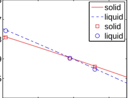
respectively. The entropies can be obtained from the slope of the Gibbs free energy – temperature curve. 1500 1600 1700 1800 −5.1 −5 −4.9 −4.8 −4.7 −4.6 Temperature (K)
Free Energy (eV/atom)
solid liquid solid liquid
Figure 1. Gibb’s free energy per atom for both the solid phase (solid line) and liquid phase (dashed line). The symbols represent data points in Broughton and Li [3] with squares for the solid phase and circles for the liquid phase.
An example is given in Fig. 1, which plots the Gibbs free energy as a function of temperature for the liquid and solid phases of Si, as described by the SW potential. The dominant source of error comes from the switching simulation between the SW liquid to the Gaussian fluid (see Appendix A for more details). This error contributes to an uncertainly of 0.884×10⁻⁴ eV/atom in the liquid Gibbs free energy, which corresponds
to melting temperature uncertainty of 0.46 K. Semiconductors and FCC metals studied here show similar error bars. The error bars of BCC metals are considerably higher, most likely due to their high melting temperature, which leads to larger statistical fluctuation.
Repeating each adiabatic switching simulation for n= 20 times usually brings the error bar of the melting point to within±1 K. The accuracy of this level can be readily achieved in a day using a computer cluster with 30 CPUs. Due to limited computational resource, enough computation is performed to reach ±1 K accuracy only for for MEAM-Si, SW-Si and MEAM-Au models. For other models, each adiabatic switching simulation is performed for only 5 or 6 times, leading to a larger error bar in the predicted free energy. The finite size of the simulation cell and small uncertainty in the determination of the equilibrium volume at finite temperature can introduce additional error to the melting point, which is not accounted for in our error estimate.
4. Summary
We have computed the melting points, latent heat, entropy and thermal expansion coefficients for nine pure elements described by four different interatomic potential models. The state-of-the-art free energy methods are used to determine the melting points accurately and efficiently, allowing a systematic comparison between the potential models. The beginning and end states and the switching paths are chosen carefully in the adiabatic switching simulations to reduce the error in the free energy calculation. The comparison reveals several systematic trends among elements with the same crystal structure. The MEAM model performs reasonably well in semiconductors compared with the SW model, and predicts more accurate thermal properties than the EAM model, especially the angular screening factor is adjusted. The original MEAM model fails to predict reasonable thermodynamic properties for BCC metals. In comparison, the FS model and the 2NN-MEAM model are more reliable for BCC metals.
Acknowledgments
We would like to thank Dr. M. Baskes, Dr. A. Caro, and Dr. G. A. Galli for useful discussions. This work is partly supported by the DOE/SciDAC project on Quantum Simulation of Materials and Nanostructures and NSF/CMMI Nano Bio Materials Program CMS-0556032. S. Ryu acknowledges the support from the Stanford Graduate Fellowship Program.
Appendix A. Error Estimates in Free Energy Calculations
In this appendix, we present some intermediate free energy results of our melting point calculations. The purpose is two-fold. First, it will enable interested readers to compare their results with ours, should they wish to adopt our computational method. Second, it demonstrates which step is the major source of error in the final estimate of the melting point. This allows further improvement of the accuracy and efficiency of melting point calculations in the future. The average and standard deviation of the reversible work
accumulated in each of the 5 adiabatic switching steps (counting forward and backward switching together) are listed in Table A1.
Step 1 corresponds to adiabatic switching from a solid phase described by an empirical potential to the quasi-harmonic approximation of itself. Step 2 corresponds to switching the solid phase along the temperature axis from T1 to T1/λ1. T1 = 1600
and λ1 = 0.8 are used for SW Si and T1 = 1200 and λ1 = 0.75 are used for MEAM Si.
Step 3 corresponds to adiabatic switching from a liquid phase described by an empirical potential to the purely repulsive liquid described by the Gaussian potential. Step 4 corresponds to adiabatic switching from the Gaussian potential to the ideal gas limit. Step 5 corresponds to switching the liquid phase along the temperature axis from T2 to
T2/λ2. T2 = 1800 and λ2 = 1.3 are used for SW Si andT2 = 1560 and λ2 = 1.3 are used
for MEAM Si. Table A1 shows that the intermediate results are similar for the SW-Si and the MEAM-Si models, both in terms of the average free energy differences and in terms of the error bars. The major source of error comes from the switching between the liquid phase and the purely repulsive liquid described by the Gaussian potential (Step 3).
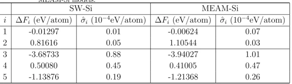
Table A1. The estimated free energy difference ∆Fi and its standard deviation in the
5 different adiabatic switching steps for the melting point calculations of SW-Si and MEAM-Si models.
SW-Si MEAM-Si
i ∆Fi (eV/atom) σˆi (10−4eV/atom) ∆Fi (eV/atom) σˆi (10−4eV/atom)
1 -0.01297 0.01 -0.00624 0.07 2 0.81616 0.05 1.10544 0.03 3 -3.68733 0.88 -3.94027 1.01 4 0.50080 0.45 0.41005 0.47 5 -1.13876 0.19 -1.21368 0.26 References
[1] S. J. Cook and P. Clancy, Phys. Rev. B47, 7686 (1993). [2] U. Landman et al, Phys. Rev. Lett.56, 155 (1986).
[3] J. Q. Broughton and X. P. Li, Phys. Rev. B 35, 9120 (1987).
[4] M. Watanabe and W. P. Reinhardt, Phys. Rev. Letter.65, 3301 (1990). [5] M. de Koning, A. Antonelli, and S. Yip, Phys. Rev. Lett. 83, 3973 (1999). [6] M. Kaczmarski, R. Rurali, E. Hern´andez, Phys. Rev. B69, 214105 (2004).
[7] MD++ source codes and automatic scripts for free energy and melting point calculations can be downloaded athttp://micro.stanford.edu/∼caiwei/Forum.
[8] F. H. Stillinger and T. A. Weber, Phys. Rev. B 31, 5262 (1985). [9] K. Ding and H. C. Andersen, Phys. Rev. B 34, 6987 (1986). [10] H. S. Park and J. A. Zimmerman, Phys. Rev. B72, 054106 (2005). [11] S. Aubry and D. A. Hughes, Phys. Rev. B73, 224116 (2006).
[12] M. W. Finnis and J. E. Sinclair, Philosophical Magazine A,50(1), 45 (1984). [13] M. I. Baskes, Phys. Rev. B46, 2727 (1992).
[14] D. R. Lide, CRC Handbook of Chemistry and Physics, 79th edition, 2007-2008. [15] M. W. Chase. Jr., NIST-JANAF Thermochemical Tables, 4th edition, (1998). [16] H. P. Hirth and J. Loath, Theory of Dislocations (1982).
[17] B. J. Lee and M. I. Baskes, Phys. Rev. B62, 8564 (2000).
[18] B. J. Lee, M. I. Baskes, H. Kim, and Y. K. Cho, Phys. Rev. B64, 184102 (2001). [19] M. I. Baskes, J. S. Nelson, and A. F. Wright, Phys. Rev. B40 , 6085 (1989). [20] M. I. Baskes, personal communications.
[21] W. Cai, C. R. Weinberger, M. I. Baskes, unpublished.
[22] V. V. Bulatov and W. Cai, Computer Simulations of Dislocations, Oxford University Press (2006). [23] C. Jarzynski, Phys. Rev. Lett.78, 2690 (1997).
[24] M. de Koning and A. Antonelli, Phys. Rev. E53, 465 (1996) [25] G. J. Martyna and M. L. Klein, J. Chem. Phys.97, 15 (1992). [26] D. A. Young and F. J. Rogers, J. Chem. Phys.80, 2789 (1984). [27] G. E. Crooks, Phys. Rev. E61, 2361 (2000).
![Table 1. Thermal properties of various elements as predicted by several empirical potentials and compared with experiments [14, 15, 16]](https://thumb-us.123doks.com/thumbv2/123dok_us/10270528.2933539/4.918.198.682.295.1049/thermal-properties-elements-predicted-empirical-potentials-compared-experiments.webp)