Return Migration and Saving Behavior of Foreign
Workers in Germany
Murat G. Kirdar
1November 16, 2005
1Email: [email protected] .I am particularly grateful to Kenneth Wolpin for his invaluable
guidance and suggestions. I have benefited greatly from advice and comments from Jere Behrman and Petra Todd, and from many helpful discussions with Dimitri Christelis, Ryo Okui, Nathan Porter and Melissa Tartari. I would also like to thank the seminar participants at Bilkent, Koç, METU and SabancıUniversities, the University of Pennyslvania and the 6th GSOEP User Confer-ence for their valuable comments. All errors are my own.
Abstract
In this paper, I develop a dynamic stochastic model of joint return migration and saving decisions that accounts for uncertainty in future employment and income and estimate this model using a longitudinal dataset on legal immigrants in Germany. The model gives a number of implications about the level, timing and selection of return migration as well as asset accumulation of immigrants according to their country of origin We also calculate the net lifetime contributions of immigrants to the pension and unemployment insurance systems of the host country. The estimated model is used to determine the impact of a number of counterfactual policy experiments on the return and savings behavior of immigrants as well as on their net contribution to the social security system. These counterfactuals include changes in the unemployment insurance program, payment of bonuses to selected groups to encourage return home, and exchange rate premiums by the source countries. In addition, I assess the impact of counterfactuals in the macroeconomic environment, like changes in wages in Germany and in purchasing power parity between Germany and the source countries.
List of Themes: Migration, Labor Market Policy
Keywords: International Migration, Unemployment Insurance, Life Cycle Models and Saving, Public Policy
1
INTRODUCTION
Many European countries see immigration as a potential solution to the social security crisis they face due to an aging native population, rising health costs and low fertility rates.1
Immigration slows down the aging of population by bringing in younger workers. Due to their age composition, immigrants are more likely to be conributing to the social security system rather than receiving benefits. In addition, return of immigrants to their home countires is significant. These immigrants pay into the social security system for many years before returning home but receive no benefits if they return before qualifying to pension benefits or little benefits even after that if they do not reside in the host country for a long time. Moreover, those who choose to stay in the host country for the rest of their lives will be drawing pension benefits for a shorter period of time because immigrants coming from less developed countries generally have lower life expectancies. However, immigrants can become a financial burden on the host country if they come at or stay until older ages because in that case they could draw from public health and social insurance systems more than they contribute to them. Moreover, if they are more likely to be unemployed compared to the natives, their withdrawal of unemployment benefits will be higher than their contributions to the unemployment insurance system. Whether immigrants become a burden also depends in part on whether the returners are selective of the most or least economically successful immigrants. One goal of this paper is to evaluate the impact of immigrants on the host country social security system by calculating their net lifetime contributions to the pension and unemployment insurance systems.
Another important policy issue regarding immigrants in many host countries is their take-up of welfare benefits. Many host countries are taking steps in the direction of restricting benefits to immigrants.2 In Germany, one reason for higher welfare participation among immigrants is their higher unemployment rate compared to that of the natives. In December 1999, the unemployment rate was 23.3% for Turkish and 18.4% for Italian immigrants in Germany. Therefore, a question of interest to policy makers is whether immigrants would be less likely to stay if the unemployment insurance system were less generous. For this purpose, 1Boerch-Supan and Schnabel (1999) report the following for the German social security system: ”In 1993, social security benefits amounted to 10.3 percent of GDP, a share more than two and a half times larger than in the United States.”
2For instance, in the U.S., a law passed in 1996 denied immigrants most types of welfare benefits. In Germany, immigrants without permanent residence may lose their right to stay if they live on welfare benefits.
I analyze how changes in the unemployment compensation system affect immigrants’ return decisions.
In order to influence the number, demographic composition and labor market status of immigrants, some host countries adopted policies to motivate immigrants to return to their home country. For instance, in 1983 Germany implemented a policy that provided financial aid to immigrants conditional on returning, especially oriented towards certain nationalities and the unemployed.3 In this paper, I also analyze the impact of variousfinancial aid schemes on return migration flows and on the demographic composition and labor market outcomes of the stayers as well as on immigrants’ net lifetime contribution to the social security system. The return behavior of immigrants has important economic implications for the source country as well. A major motivation for immigration is asset accumulation. Although an exodus of workers seeking to take advantage of higher wages in other countries may impose a cost on the source country economy, migrants who return home often bring with them significant amounts of assets. Moreover, many of them invest their assets in small businesses.4
I calculate the amount of wealth that enters the source country with the returning migrants and evaluate the impact of source country policies aimed to increase this amount.
This paper develops and estimates a dynamic model of joint return migration and savings decisions under uncertainty. In the model, migrants are subject to earnings, employment and preference shocks and they make decisions about what fraction of their income to save and about whether and when to return to their home country. The structural framework of the model allows us to evaluate the impact a number of counterfactual policy experiments. In addition, since I model the migrants’ decisions in a dynamic setting, I am able to explore the effects of these policies not only on migrants’ return decision but also on their duration of residence. The model also incorporates unobserved heterogeneity in migrants’ permanent skill endowments and preferences.
In the model, the reasons that immigrants return to their home country are higher pur-chasing power of accumulated assets in the home country due to lower prices there and immigrants preference to live in their home country rather than in Germany. I exploit the variation in the price levels across source countries to identify the effects of purchasing power on immigrants’ decisions. I also investigate how counterfactual changes in the purchasing 3Dustmann (1996) reports that the return aid amounted to 10,500 DM for each worker. In addition, there was a 1,500 DM bonus for each child. (Roughly, 2 DM is equal to 1 US $.)
4Dustmann and Kirschkampf (2002) report that, based on a sample of Turkish return migrants, 51 percent operated small businesses.
power parity influence immigrants’ savings and return decisions. The model also incorpo-rates variation in the earnings potential across the source countries. This would be especially important in the return decision of younger immigrants. I assess the response of immigrants to changes in the wage differential between the source country and Germany.
The model is estimated using a unique longitudinal dataset from Germany that contains information on legal immigrants from five different countries, which include EU member as well as non-member countries. The pieces of information employed from the dataset include immigrants’ labor market status and earnings as well as their return migration and saving choices. In the estimation of the model, a simulated maximum likelihood technique is used. The results indicate that the model can account very well for the key features in these four pieces of information according to EU status.
The model provides a characterization of immigrants’ return and saving behavior by country of origin. 61 percent of Turkish, 31 percent of ex-Yugoslavian, 88 percent of Greek, 83 percent of Italian and 92 percent of Spanish immigrants return to their home countries during their lifetime. The hazard function of non-EU immigrants is hump-shaped and peaks around 15 years of residence whereas EU immigrants’ hazard function is initially a fast-decreasing one that levels off after 10 years of residence before rising slightly again at retirement. The savings profiles of both immigrant groups are downward-sloping. It is steeper for non-EU immigrants, though. Both EU and non-EU immigrants save one third of their income right after arrival. The saving rate gradually drops to 10 percent in the next 20 years. It keeps dropping for non-EU immigrants and the savings rate averages around zero after 30 years of residence whereas for EU immigrants it stays at around 10 percent from 20 to 30 years of residence, then gradually drops to around 5 percent.
This paper provides the first estimate, to my knowledge, of the amount of wealth that return migrants bring to their home country. I find that Turkish return migrants take on average 92,857 DM, ex-Yugoslavians 91,407 DM, Greeks 94,093 DM, Italians 42,619 DM and Spanish 84,129 DM to their home countries. Using information on the total number of Turkish return migrants between 1993 and 1998, I estimate that the total amount of returned wealth to Turkey was almost a billion DM per year in this time interval.
Using the estimates, I calculate the net contribution of immigrants to the pension and unemployment insurance systems by country of origin and age at entry. Immigrants from all
five countries of origin, in particular those coming from non-EU countries, make positive net lifetime contributions to the pension insurance system. This ranges from 5,662 DM for Greek
immigrants to 21,461 DM for Turkish immigrants. On the other hand, net contribution to the unemployment insurance system is negative for non-EU immigrants. It stays positive for EU immigrants, though. When I examine the total net contributions to these two systems, I find that all four nationalities but ex-Yugoslavians make positive net contributions. For ex-Yugoslavians, the net contribution is -1,095 DM. The positive net contributions ranges from 5,844 DM for Turkish immigrants to 11,712 DM for Spanish immigrants.
An important contribution of this paper to the literature on immigrants’ impact on the host country social security system is that it analyzes net contributions of immigrants when return migration is a choice. In fact, I show that treating return migration as an exogenous factor causes a serious underestimation of net lifetime contributions.
In a policy experiment, I show that the German government can in fact increase the net contributions to these two insurance systems by providing financial bonuses to the un-employed conditional on return. This policy is more effective on non-EU immigrants. For non-EU immigrants, I find that the optimal amount of bonus is in the 45,000 to 50,000DM range regardless of the duration of residence at which the bonus is received when the bonus is given at one point in time. The impact of the policy in decreasing unemployment rate of immigrants is significant at the time the policy is implemented. However, the fall in the unemployment rate diminishes over time. When such a policy is kept in effect all the time rather than at a single point in time, net contributions to the two insurance systems can still be increased. In this case, upper limits on age or duration of residence for qualification would be needed in order to prevent the immigrants from first receiving the unemployment benefits then taking the bonus before retirement and leaving.
I also examine the impact of a policy that restricts the generosity of the unemployment insurance system, which is the elimination of unemployment assistance —the second phase of the benefits—. Given the high unemployment rates of immigrants in Germany, a less generous unemployment insurance system.could increase the return rates of immigrants. However, I
find that this policy has a very small impact in terms of increasing the return rates of immigrants.
In another policy experiment, I assess the impact of an exchange rate premium provided by the source country governments on the amount of assets that immigrants take with them when they return to their home country. Such policies have been used by various source countries in order to boost the amount of returned wealth. Even though this policy increases the fraction of returners, it also decreases the amount of average asset holdings of a returner
because the average duration of residence of returners shortens. Moroever, the latter affect dominates the former and the amount of returned wealth from all emigrants from the source country decreases.
The way immigrants’ return and savings choices respond to counterfactual changes in the macroeconomic environment is also analyzed. The variables of the macroeconomic environ-ment influencing immigrants’ return and saving decisions are wages in Germany, expected wages in the home country and purchasing power parity between the home country and Germany. Whenever the theoretical impact of a change in these variables is ambiguous, the counterfactual simulations allows us to find out the empirical answer. For instance, an increase in German wages has conflicting income and substitution effects on the return de-cision. I find that substitution effect dominates and immigrants become more likely to stay. On the saving decision, an increase in ppp has conflicting income and substitution effects. In this case, Ifind that the income effect dominates and immigrants save less.
Next section provides background information, reviews the relevant literature and high-lights the main contributions of this paper. In section 3, the model and its solution is described. Section 4 presents the data and some descriptive analysis. Section 5 covers the estimation method and section 6 presents the estimation results. The implications of the results as to the host country social security system and the return of wealth to the home country along with the returning migrants is examined in section 7. The results of policy experiments and the counterfactuals on the macroeconomic environment are presented in sections 8 and 9, respectively. Section 10 concludes.
2
BACKGROUND AND RELEVANT LITERATURE
This study analyzes the behavior of the guestworkers of 1960’s and 70’s who immigrated to Germany under the bilateral agreements signed by the German government with 5 Mediter-ranean countries. (3 European Union countries: Greece, Italy and Spain; and 2 non-EU countries: Turkey and ex-Yugoslavia). The German government actively recruited immi-grant workers by opening recruitment posts in the capitals and major cities of these coun-tries. Residents of these countries who were willing to go to Germany registered at these agencies and were matched with employers in Germany. The initial goal of the guestworker recruitment system was to have these migrants work in Germany for a limited number of years and replace them with new ones once their permit expired. While most of the migrants
in fact went back, some stayed. Paine (1974) reports that, in practice, if these guestworkers maintained their employment status in Germany for a few years, they were able to stay. In 1973, after the oil price shocks, recruitment of new immigrant workers came to a halt. However, immigration continued mostly in the form of family reunification.5
Immigrants constitute a relatively significant part of the German work force. The Federal Ministry of the Interior reports that “1.95m foreigners had a job that made them liable to pay social security contributions in the western federal territory, meaning they account for 8.9 per cent of all gainfully employed persons.” Return migration of these immigrants has remained at a significant level. Between 1993 and 1998, around 45,000 Turks returned to Turkey each year on average (Federal Ministry of the Interior). Given that there are around 2 million Turkish immigrants in Germany, this roughly amounts to a 2% annual hazard rate. The literature has identified a number of determinants of return migration. Borjas and Bratsberg (1996) emphasize that return migration may be part of an optimal life-cycle loca-tion decision. At the time they immigrate, migrants realize that after they acquire physical or human capital in the host country, it may be optimal for them to return because the returns to that type of capital are higher in the home country. The assets that guestworkers accumulate in Germany have higher purchasing power at the home country due to the lower prices there. On the other hand, since most guestworkers took jobs as unskilled workers, it is quite unlikely that their goal in moving to Germany was to acquire human capital. Even if they acquired some skills, these skills would be specific to the German labor market, which is a more capital-intensive production environment, and would not fit to the needs of the home country labor market. In fact, based on a survey of Turkish emigrants from Germany in Turkey, Dustmann and Kirchkamp (2002) report that only 6 percent worked as salaried workers after return whereas 51 percent of the returners were self-employed. The other 43 percent were retired. Another interesting fact that Dustmann and Kirchkamp report is that the median age of the retirees among the returners was 45. This suggests that some im-migrants were able to accumulate enough assets by a relatively early age to spend the rest of their lives as rentiers. The facts that half of these migrants engaged in entrepreneurial activities after return and that most of the rest lived as rentiers suggest a savings motive for immigrating to Germany. If the goal of guestworkers were to accumulate assets, they would have high saving rates. Based on a empirical investigation of Turkish households in Germany, Kumcu (1989), in fact,finds evidence for very high savings rates. Another reason
for return migration, noted by Hill (1987), is that migrants have a preference for location. Return migration may also be the result of unexpected events, either in the host country or in the home country (Berninghaus and Siefer-Vogt, 1992). Unexpected changes in earnings or in preferences for living in Germany, for instance due to the death of family members back at home, might alter immigrants’ decisions.
There is very limited empirical evidence concerning the relationship between savings and return migration. The existing empirical papers on the savings behavior of immigrants, Merkle and Zimmermann (1992), Kumcu (1989), treat return migration as exogenous. How-ever, Dustmann (1995) shows that treating return decision as exogenous in analyzing the savings behavior of migrants could give false implications in policy experiments. The re-search on the joint return and savings decisions of immigrants has been theoretical so far. Berninghaus and Seifert-Vogt (1992) provide a theoretical analysis of optimal savings and return migration strategies in a stochastic dynamic model where the cause of return is higher purchasing power parity. In a similar but more extended model, I conduct thefirst empirical analysis of this joint saving and return migration decisions.
There has been a number of studies involving the impact of immigrants on the host country social security system. Analyzing the redistribution caused by public transfers, old-age pensions, and tax and social security contributions in the German context, Buchel and Frick (2001)find that immigrants are net payers. They attribute this fact mainly to the age composition of immigrants, which makes them less likely to receive old-age pensions. This study examines net contributions in a few years and therefore is likely to be influenced with the particular age composition or labor market situation in that few years. On the other hand, this study conducts a longitudinal analysis; therefore, it accounts for the changes in immigrants’ contributions over their life cycle. Lee and Miller (2000), using detailed demo-graphic and fiscal environment projections, calculate the net fiscal impact of immigration over the life-cycle and generations in the U.S andfind that the impact of changing the level of immigration would be rather small. However, using similar aggregate demographic and employment projections to calculate the contribution rate to the social security system un-der various migration scenarios that would keep the budget of the pension system balanced, Borsch-Supan (1994) finds that immigration reduces the increase in the contribution rates by 50 percent and that the positive impact of immigration through the alleviation of depen-dency ratio dominates the negative impact of immigration through its depressing effect on the wages. In a calibrated overlapping generations general equilibrium model, Storesletten
(2000) finds the annual immigration necessary to balance the government budget as well as the net present value of admitting an immigrant. Unlike Lee and Miller, he finds that the quantitative impact of immigration on the fiscal policy can be significant and under certain immigration policies it would be possible to sustain currentfiscal policy.
Unlike the above mentioned studies whose findings are based on calibrated values, my results come from a maximum likelihood estimation in which I use a rich longitudinal dataset and to my knowledge, this is the first estimated structural model of migration behavior and its impact on the host as well as source countries. In order to estimate my model, I had to keep it simpler, though. For instance, I ignore the indirect effects on wages and on native productivity. However, empirical studies conducted so far on this issue found that there is no evidence for immigrants depressing the labor market conditions for natives. Friedberg and Hunt (1995) in their survey of the impact of immigration on the host country and Lalonde and Topel (1991) point out that the effect of immigration on equilibrium wages is negligible. Moreover, given the rigid institutional features of the German labor market, this becomes even more likely. On the other hand, one might expect the impact on the employment of natives to be more important. However, Piscke and Velling (1997) find no employment displacement effects of immigration on natives in Germany. Therefore, I think that a partial equilibrium approach for this study is appropriate.
I also limit the analysis to first-generation immigrants only. An intergenerational exten-sion of this study would require modeling fertility choices of thefirst-generation immigrants, which would severely increase the computational burden. On the other hand, I also intro-duce more general modeling features. All of above-mentioned studies on thefiscal impact of immigration take return migration as exogenous. However, return migration is very much linked to household income and labor market status and this has important implications for the net fiscal impact of immigrants. For instance, fiscal impact will be more positive when immigrants who are less successful in the labor market are more likely to return compared to that under a random outflow of immigrants. Moreover, it will also be important whether immigrants are more likely to return in the early periods or in later periods in calculating their net contributions. By explicitly modeling the return migration choice, I am able to account for the effect of the timing as well as selection in return migration on the net con-tributions of immigrants. I also add a new dimension to the studies on the fiscal impact of immigration.by examining policies from the return perspective. I analyze the results of a number of policies aimed at altering the selection process in return migration in order to
increase the net contributions of immigrants to the pension and unemployment insurance systems.
3
THE MODEL
In this section I present the basic structure of the model and its solution in the dynamic setting.
3.1
Basic Structure
The basic structure is the discrete choice dynamic programming approach, as outlined in Eckstein and Wolpin (1989). Immigrants choose among a finite set of mutually exclusive alternatives over a finite horizon. I model the decisions of male household heads.
3.1.1 Choice Set
The elements of the choice set are return migration and savings decisions. Each period, immigrants realize their labor market status and earnings and decidefirst whether to stay in Germany or go back to their home country. If they choose to stay, they also make a decision about how much to save.
3.1.2 Preferences in Germany
Immigrants have preferences over consumption(ct)and location of residence. Their marginal
utility of consumption (µ) varies by their labor market status (lt), age and their permanent
unobserved preference characteristics.6 Below, ρ(.) stands for immigrants’ psychic cost of
living in Germany. This is the difference between the psychic utility in Germany and that in the host country. Immigrants’ pyschic cost varies by their duration of residence in Germany, as they adjust to the new surroundings, as well as by their age at entry and unobserved permanent characteristics.
ut(.) =µ(lt, aget, type)
c1t−λ
1−λ +ρ(t, age0, type) exp(η
s t)
6Individuals are allowed to differ in their permanent unobserved characteristics as well as in their observed characteristics. We group the immigrants into a finite number of types according to these unobserved characteristics and assume that immigrants within a type group share the same unobserved heterogeneity.
Above, λ is the constant relative risk aversion parameter and ηs
t is a random shock to
preferences.
Constraints Given their net earnings (yt) and asset income(rAt), immigrants make their
consumption and saving decisions. At is asset holdings at period t and cmin is the minimum consumption level, which is equal to the subsistence income set by the German government. In this model, minimum consumption level is an institutional feature because this consump-tion level is guranteed by the German government through its social assistance for subsistence income program. I allow this subsistence income, which depends on family size, to vary by age and nationality (z). (This is explained later in the social assistance subsection.) In addition, borrowing is not allowed.7
ct+ (At+1−At) ≤ yt+rAt
ct ≥ cmin(aget, z)
At ≥ 0
3.1.3 Labor Market Status in Germany
I assume that all male household heads who are not retired are willing to work. Therefore, whether they are unemployed or employed depends only on whether or not they receive job offers.
There are three potential paths to retirement: 1) One can retire after age 65. 2) Retire-ment is also possible at age 63 conditional on having a long service life, which is 35 years. 3) Conditional on a qualifying period of at least 15 years, workers who have been unemployed for 52 weeks can retire at age 60.8
If an immigrant does not qualify for retirement according to the above rules, random job offers determine whether they are employed (l = 1) or unemployed (l = 0). The job offer probability, (lt)varies according to the labor market status in the previous period, age, age
at entry to Germany, nationality as well as permanent labor market characteristics.
lt=L(lt−1, aget, age0, z, type) 7Immigrants are there to save.
8We assume that this structure is unchanged during the life-cycle of an immigrant (In fact, there were a slight upward adjustment in the retirement age.) and that immigrants expect no change.
Once one of the above three retirement rules becomes applicaple, immigrants may enter retirement(l = 2), which is an absorbing state. Employment status in this case is modeled using a multinomial logit.
3.1.4 Income in Germany
Gross Earnings Labor market earnings of an immigrant at period t, yt, depends on how
much human capital he has acquired and on the rental price of human capital, p. The level of human capital at any period, Ht, depends on the years of residence, age at entry,
nationality and permanent skill characteristics of the immigrant. In addition, there is a random productivity shock,.ηyt.
yt = pHtexp(ηyt)
Ht = H(t, age0, z, type)
Social Security Contributions Workers in Germany pay three types of social security contributions: pension insurance, unemployment and health insurance premiums. Pension insurance contribution is applied at a rate of 9.35%(τp) and unemployment insurance con-tribution is applied at a rate of 2.15% (τu), both up to a earnings maximum of 85,000DM
(ymax) (1998 prices). The health insurance contribution is applied at a rate of 7% (τh) up
to a earnings maximum of 0.75ymax (in 1998 prices). Earnings below 6,000DM (ymin)(1998 prices) are exempt from social security taxes.910
Γ(yt) =
0 if yt≤ymin
(τp+τu+τh)y
t if ymin < yt≤0.75ymax
(τp+τu)yt+τhymax,1 if 0.75ymax< yt≤ymax
(τp+τu)ymax,2+τhymax,1 if ymax,2 < y
t
(1)
Net Earnings Net earnings, yt is gross earnings net of social security contributions and
income taxes.
yt= (1−τ[yt−Γ(yt)]) [yt−Γ(yt)]
9When earnings is below the tax-exempt level, employer still makes a insurance contribution and this period counts toward pension qualifying period for the worker.
10There has been very small changes in the social security contribution rates. We assume that immigrants expect the contributions rates to stay at this level when they make forecasts about the future in the forward-looking nature of the model.
Above, τ[yt−Γ(yt)]is the average income tax rate for yt−Γ(yt), earnings net of social
security contributions. τ(.) is calculated according to following marginal tax rate schedule: Income below subsistence income is tax free. Above that level, the marginal tax rate rises from 22% to 56% up to an earnings level of 120,000DM (in 1998 prices)11
Unemployment Benefits and Unemployment Assistance Immigrants who worked for at least 360 days in the last 3 years can receive unemployment benefits, which are equal to 67% of their last net earnings if they have at least one child. The entitlement duration varies from 180 to 960 days depending on the age and experience of the worker. However, there is a second phase of the unemployment insurance system. Workers who are no longer eligible for unemployment benefits can receive unemployment assistance. This is equal to 57% of their last net earnings if they have at least one child and there is no limit to the duration of unemployment assistance after the exhaustion of unemployment benefits.
For tractability, I take unemployment benefits and assistance at any period as the above percentages of expected net earnings at that period rather than as percentages of the real-ized last net earnings.12 In addition, I take the duration of entitlement to unemployment
benefits equal to two years (which is equivalent to one period in the solution of the model). Therefore, an immigrant who is unemployed for two consecutive periods receives unemploy-ment assistance instead, which is ten percent less. Moreover, unlike unemployunemploy-ment benefits, unemployment assistance is means tested according to asset income. Both unemployment benefits and assistance are net earnings and, therefore neither social security nor income taxes are applicable.
11These numbers are chosen to average the values for the years 1965 to 2000. Even though there has been changes in these values, they were small in magnitude.We assume that immigrants do not expect any changes in the marginal tax rate schedule in the future when solving the forward-looking model.
12There is an additional approximation here in that taxes are calculated based on expected earnings. Expected value of taxes could be different from taxes calculated based on expected earnings due to the kinks in the tax function.
yt =
0 if not qualified for benefits
0.67³pHteσ 2 y/2−Γ(pH teσ 2 y/2) ´ h 1−τ³pHteσ 2 y/2−Γ(pH teσ 2 y/2) ´i if (lt= 0 and lt−1 = 1) 0.57³pHteσ 2 y/2−Γ(pH teσ 2 y/2) ´ h 1−τ³pHteσ 2 y/2−Γ(pH teσ 2 y/2) ´i −rAt
if (lt = 0 andlt−1 = 0 and qualified for benefits)
Immigrants who have never been employed since their entry to Germany do not qualify for unemployment benefits. I assume that after 4 years of residence, all immigrants qualify for unemployment benefits. In other words, residence in the host country without work experience can not last more than 4 years.13
Pension Benefits German pension insurance system is mandatory to all workers except for the self-employed and those with very low incomes. For these two groups, which is a small fraction of the immigrant population, I assume that they choose to enroll in the pension insurance system.
The minimum contribution period to qualify for pension benefits isfive years in Germany. Since periods of unemployment are included in the qualifying period in the German pension insurance system and in the model all immigrants are willing to work, everybody with a duration of residence longer than the qualifying period is entitled to pension benefits.
Pension benefits in Germany depend on workers’ history of labor market earnings and on their duration of contribution. The replacement rate, defined as pension benefits over average net earnings of all employed workers, for a worker with forty-five year earnings history and average lifetime earnings is 72 percent. In addition, pension benefits are proportional to duration of contribution. Therefore, for the worker with average lifetime earnings, each additional year of earnings history amounts to a 1.6 percent increase in the replacement rate. For tractability, I generalize this property for the worker with average lifetime earnings to all workers. This assumes that the replacement rate does not depend on the relative income level of workers, i.e. there is no redistribution. Borsch-Supan and Schnabel (1999) 13It would be impossible to maintain residence status after 4 years of unemployment for non-EU immi-grants. Moreover, many of the guestworkers were already assigned to German employers at the time of entry. Besides, further residence after 4 years of unemployment would be very unlikely for any economic migrant with zero earnings.
report that there is in fact very little redistribution in the German pension insurance system, except for those with very high incomes —those whose income are three times as much as the national average—. Given the relatively low incomes of immigrants in Germany, there is a very tiny of fraction of them in this income range.
Again for tractability, in calculating pension benefits at period t, I assume that replace-ment rate is applied to the average of expected net earnings at all periods until period t rather than to the average of realized net earnings. Below, yet is this baseline earnings position to
which the replacement rate of 0.016t is applied.
e yt= t X j=1 ³ pHteσ 2 y/2 −Γ(pH teσ 2 y/2) ´ h 1−τ³pHteσ 2 y/2−Γ(pH teσ 2 y/2) ´i t
Pension beneficiaries do not pay contributions to the pension or unemployment insurance systems. Only health insurance contributions,ΓH, according to the rules in equation 1 above,
are applied. Pension beneficiaries do not pay income taxes either. Thus, pension benefits can be written as follows:
yt= 0.016tyet−ΓH(yet) if lt = 2 and t≥5 years
Social Assistance for Subsistence Income Immigrants can also receive social assistance if their income is not high enough to provide for their basic needs. Eligibility depends on net income and asset holdings. If the sum of monthly net income and assetflows of residents falls below the subsistence income level14, the government makes up for the difference. Subsistence
income for a family depends on its size and varies across states. In 1998, the payment for the head of the household averaged around 520 DM across states. The spouse of the household head receives 80% of this amount and there is an additional payment for each child, that varies from 50% to 90% depending on the age of the child.
Marriage status and the number of children are not included in the model as state vari-ables. However, marriage status and number of children is strongly correlated with age and nationality. Therefore, I write the subsistence level income as 520DM times a family multiplier that varies by age and nationality. The dependence of the multiplier on age and nationality is estimated outside of the model. Details of the calculation of this multiplier is 14According to the German Ministry for Health and Social Services, this subsistence income includes expenses on food, housing, clothing, toiletries, household goods, heating and everday personal necessities, and -within resonable limits- expenses for socializing.
provided in Appendix C.
yt+rAt>= 520∗f amily_multp(aget, z) DM per month
3.1.5 Preferences in the Home Country
Once an immigrant returns to his home country, he exits the panel. As a result, I have no information on his labor market status, earnings or savings decisions after return. Therefore, the utility an immigrant receives from returning to his home country to spend the rest of his life there, VL( Set),is written as a function of a subset of the state variables at the time
of return. These state variables include assets interacted with purchasing power parity, age, duration of residence and nationality. This part of immigrants’ preferences is deterministic.
VL(Set) =VL(pppAt, aget, t, z)
This function is explained in detail in Appendix A along with the other functional spec-ifications.
3.2
The Problem in Recursive Formulation
Given the current realizations of the shocks to their earnings and preferences, immigrants calculate the value of staying in Germany, VS
t (St), and the value of returning to the home
country, VtL( Set), and make their return decision accordingly. St is the state space at time
t. The decision spell starts when an immigrant enters Germany and goes until he dies or returns to his home country. Mortality is deterministic and the age of mortality is taken as 70 for Turkish immigrants, 72 for Yugoslavian and 76 for Italian, Greek and Spanish immigrants in accordance with life expectancies for males in these countries.
Vt(St) = max{VtS(St), VtL( Set)}
If immigrants choose to stay in Germany, they make a saving decision over K alternatives to maximize the present discounted value of their remaining lifetime utility.15 Below dk
τ = 1
if alternative k is chosen at period τ and =0 otherwise. δ is the discount factor. The expectation is taken over the distribution of shocks to earnings and preferences.
VtS(St) = max ∆Ak t E " T X τ=t K X k=1 δτ−tukτd k τ|St #
15The saving choice is discretized into 10 separate values, which are ±(10,000, 20,000, 30,000) and 0, +40,000, +50,000 and +60,000.
The above problem can be recast in the following dynamic programming form.
VtS(St) = max At+1{
u(At+1,ηt) +δEtVt+1(St+1)}
The solution to this problem is given by a decision rule that takes the points of the state space to the optimal saving choice. In the last period of the problem, the continuation value is a bequest function that depends on the level of assets and the permanent preference characteristics.
VT+1(ST+1) =B(AT+1, type)
The solution of the problem is not analytic and a numerical backward solution algorithm is used. One peculiar thing about this problem is that its solution involves the calculation ofEtVt+1(St+1), which requires calculation of multi-dimensional integrals due to the number of stochastic elements in the model. This is calculated using Monte-Carlo integration over the joint distribution of shocks to preferences and earnings at all possible points of the state space for all periods. Since the number of the state space points at which the problem needs to be solved depends on the decision horizon, I take the decision period as two years to alleviate the computational burden.
4
DATA
The dataset used in this study is the German Socio-Economic Panel (GSOEP). This is a longitudinal dataset of households in Germany that contains an oversampled group of immigrants fromfive Mediterranean countries, of which three are members of the European Union (Greece, Italy and Spain) and two are not (Turkey and Ex-Yugoslavia). I use the 2000 version of the GSOEP, which is conducted annually from 1984 to 2000. The initial sample contains 1326 households.
I analyze the behavior of male immigrants who made the choice to immigrate to Germany. Therefore, I restrict the sample to households with a first-generation immigrant male. A
first-generation immigrant is defined as one who entered Germany after the age of 18. 1055 households have a first-generation male household head. In addition, 9 households have a
first-generation male whose family status is registered as a spouse. Defining these 9 males as household heads, I end up with 1064 households with afirst-generation male household head. Two of these are dropped because these male household heads entered Germany after the age
of 50. Consequently, thefinal sample contains 1062 malefirst-generation household heads.16
The surveys on these household heads contain detailed information on return migration, savings, labor market status and earnings.
Return migration is reported as "moved out of country" in the sample by information gathered from other family members, relatives, neighbours, and so forth. Of course, it is possible that some of these immigrants were elsewhere in Germany but mistakenly reported as "moved out of the country". The model incorporates this possibility by allowing for classification error in return migration outcomes.
Savings information is available only after 1991. Immigrants are asked about their monthly savings. However, they are not asked about their dissavings; therefore, the data is censored at zero. Since the saving choice can take negative values in the model, I treat the zero saving values in the data as zero or negative in the estimation.
Information on immigrants’ labor market status is available from their year of entry to Germany. The part from their year of entry to 1983 is available in a yearly form, gathered from retrospective questions. The data on labor market status after 1983 is available in a monthly form I also have information on income annually from 1983 on, including amounts for each type of income. In accordance with the sources of income in the model, I use labor income, unemployment benefits and assistance, pension benefits, subsistence income and asset flows components. All the income data in the paper are reported in 1998 prices.
The initial sample of immigrants is a random sample of the immigrants in Germany in 1984. Since some immigrants already returned to their home country by 1984, this is not a random sample of the initial cohorts of immigrants. Therefore, the information on their return behavior, for instance, within thefirst ten years only comes from the immigrants who entered Germany after 1975. (The first return observed is in 1985.) This implies that when I compute the Kaplan-Meier hazard functions for return, I assume that there are no cohort effects.
Another issue in the data with regard to the model is that there is no information about asset holdings, which is a state variable of the model. To deal with this problem, I use a particular estimation method that solves the problem of missing state variables in dynamic 16In addition, there are 28 other first-generation males who enter the sample later, after 1984, mostly through marriages to the initial members of the sample. However, since this group is a selected sample of immigrants who entered Germany after 1984 through their higher propensity to marry, we exclude this group.
panel data models.
Macro data are also used in the estimation. These are the purchasing power parity of the source countries with Germany, which determine the purchasing power of accumulated wealth in Germany, and the ratios of expected wages in the source countries, which is used as a measure of the relative attractiveness of the labor markets in the source countries. In calculating the expected wages, unemployment rates and replacement rates of unemployment benefits in the source countries are taken into consideration. Since there is no calendar year in the model, averages of time series data are taken.17 The macro data are displayed in Table
4.1.
4.1
Descriptive Statistics
Figure 4.1.1 illustrates the employment probability and mean income according to duration of residence by EU status. For both EU and non-EU immigrants, employment probability drops significantly by duration of residence. Analyzing this by age-at-entry cohorts reveals that this is caused by the aging of immigrants rather than duration of residence per se. The downward profile is much more prominent for non-EU immigrants. The income profiles in Figure 4.1.1 indicate that per period income levels lie between sixty thousand and
seventy-five thousand DM. There is no significant difference in income levels according to EU status. EU immigrants have only slightly higher income levels. In the few last periods, as immigrants retire, income levels drop. The profile is rather flat for both EU and non-EU immigrants. Despite increasing unemployment rates, income levels are not decreasing. Table 4.1.1 displays the transition into retirement for all immigrants. The earliest age of retirement is sixty, at which 37 percent of immigrants enters retirement. At age 66, ninety-two percent of the immigrants are already retired. Retirement information is not disaggregated to EU status level due to limited number of observations at these ages.
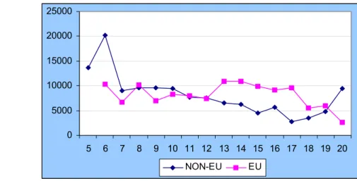
Mean non-negative savings profile18according to EU status is illustrated in Figure 4.1.2.19
17One could argue that not having calendar time, we could miss the impact of a time trend in the macroeco-nomic conditions in the source countries. In particular, this is the case for Spain which saw an improvement in labor market conditions after joining the EU. However, these changes would be much less important for older generations and most of the Spanish guestworkers were beyond their prime-age when the positive changes in Spanish labor market took place.
18This is mean non-negative savings because savings data are censored below at zero.
19Since the savings data is available only after 1991, the earliest savings observation we have is at thefifth period.
The most prominent feature of thefigure is the difference in the shape of the profiles according to EU status. There is a significant decrease in the mean non-negative savings of non-EU immigrants over duration of residence while that of EU immigrants seem to be relatively constant over time. This is not caused by the differences in their income profiles; their income profiles as can be seen in Figure 4.1.1 are very similar. Between the 5th and 10th periods, non-EU immigrants save on average more than EU immigrants whereas after the 12th period, EU immigrants save more.
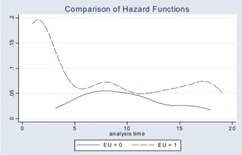
Figure 4.1.3 displays the smoothed Kaplan-Meier hazard contributions according to EU status20. EU immigrants are more likely to return. A comparison of the survivor functions
by EU status reveals that they are significantly different. There are important diffferences in the timing of return as well. EU immigrants are much more likely to return in the earlier periods. Their hazard rates drop precipitously in the first five periods and after that their hazard rates pretty much smooths out at a six percent level, with a slight rise as immigrants reach retirement age. On the other hand, for non-EU immigrants the hazard function has a hump-shape that peaks at around the 7th to 8th periods (15 years of residence) at a level of
five and a half percent.
5
ESTIMATION METHOD
The observed outcomes in the data are return migration choice(mt),savings choice(At+1−
At),earnings of the migrant(yt),and the labor market status of the migrant(lt).Let{Oi}=
{Di, Xi} denote observed outcomes for individual i, where Di = {dit} = {{mit},{Ait −
Ait−1}}is the history of observed choices andXi ={xit}={{lit},{yit}}is the history of
ob-served exogenous covariates. The data areOobsi ={{mit}Tt=1i ,{Ait−Ait−1}tT=iti,1991,{lit}
Ti
t=1,{yit}Tt=iti,1983} where ti,19xx is the period number for individual i in 19xx and Ti is the last period in the
sample for individual i. If the return choice is to leave, in the last period, Ti, the other
outcomes are not observed.
One of the endogenous state variables, assets, is not observed. Therefore, I use the method introduced by Keane and Wolpin (2001) for estimating dynamic panel data models with unobserved endogenous state variables. Typically, calculation of the probabilities that form the likelihood function requires conditioning on past state variables. The novel feature 20This is based on a weighted kernel smooth of estimated hazard contributions. A relatively narrow bandwidth is chosen in order not to smooth to much.
of this method is that it obviates the need to calculate these conditional probabilities. The underlying idea of this estimation method is to minimize the distance between the simulated and reported outcomes. A measure of the distance between the simulated and reported outcomes is constructed by assuming that the observed outcomes are measured with error. In a recent paper, Keane and Sauer (2003) show that this estimator has good small sample properties in a more extended setting.
The key assumption, therefore, is that the observed outcomes are measured with error. By acknowledging the existence of measurement errors (classification errors in the case of discrete outcomes), I incorporate into the likelihood calculation, for instance, the fact that when a migrant is observed as employed, there is a positive probability that he was in fact unemployed, but his employment status was classified incorrectly in the data. In the case of observed earnings and savings, I take a similar approach; however, in this case the measurement errors have continuous distributions.
5.1
Generation of Simulated Outcomes
Using the initial state variables, {A0 = 021, l0 = 122} and the sequence of random shocks
drawn for each individual and period, I simulate N choice histories, Dsim =
©
{mt,(At+1−At)}Tt=1i
ªN
n=1, and histories for exogenous covariates,X
sim =©
{et, yt}Tt=1t
ªN n=1for each individual i. Unbiased classification errors are also constructed using these simulated values. (See Appendix B for the specifications of these classification errors.)
5.2
Likelihood Function
L(Θ) = I Y i=1 P(Oobsi |Θ)The contribution to the likelihood of individual i is calculated by the below simulator, which is the probability of observing the reported outcomes conditional on the simulated outcomes averaged over the N simulated choice histories. This simulator is conditional on staying in Germany until 1984 because the sample contains only immigrants who stayed in 21Since most of these immigrants are unskilled young people from poor regions that chose to work in a foreign country, we assume that their initial wealth is zero.
22Since employment transition is a first-order Markov chain and that most immigrants were employed in their first period in Germany —being guestworkers, they were already assigned jobs before entry—, this restriction that everybody was employed before entry would have very little impact on the results.
Germany until 1984. b P(Oiobs) = N P n=1
P((Diobs, Xiobs)|(Dinsim, Xinsim), I({mint} ti,1983 t=1 = 0)) N P n=1 I({mint} ti,1983 t=1 = 0) Note that P((Dobs
i , Xiobs)|(Dsimin , Xinsim) is not conditional on any of the state variables.
Therefore, this probability can be calculated even when some of the state variables are not observed.
Unobserved heterogeneity enters the estimation in the following way: Following Heckman and Singer’s (1984) non-parametric modeling of unobserved heterogeneity, I assume that there is a finite number (K) of type groups. Each individual i may belong to any of these type groups, 1 to K. It is the probability of being a certain type that differs across individuals. Therefore, when I generate the simulated outcomes for individual i and calculate the above simulator, I do it separately for all types. Then, the likelihood contribution for this individual is calculated as the weighted average of the above simulator over the probabilities of his belonging to each type.
b P(Oiobs) = K X k=1 κi,k N/KP n=1
P(Oiobs)|(Oiknsim), I({mit}tt1983=1 = 0))
N/KP n=1 I({mit}tt1983=1 = 0)
where κi,k, the probability of individual i being of type k, is specified as a logit with age
at entry and country of origin as arguments.
κk =κ(age0, z, t1983)
The probability of observing the reported spells conditional on the simulated spells can be written as follows: P((Dobs
i , Xiobs)|(Dinsim, Xinsim)) = P(Miobs|Minsim)
QTi
t=1Pr(Ait −
Ait−1)obs|(Aint−Aint−1)sim] Pr(yitobs|ysimint) Pr(lobsit |lsimint).
Measurement error distributions and classification error rates are used to calculate these probabilities. See appendix B for these calculations. For the optimization method, the Downhill Simplex Algorithm is used.
6
RESULTS
In this section, maximum likelihood estimation results based on the full solution of the dynamic model are presented.
6.1
Model Fit
I first illustrate and discuss how the model’s predictions as to the return migration and savings choices as well as the exegenous transitions fit the observed features of the data. Figure 6.1.1 compares the actual and predicted hazard functions for non-EU immigrants. The model captures both the level and timing of return migration very well. In fact, the predictions are almost identical to the actual values. Model predictions of the hazard rates of EU immigrants are compared to the actual values in Figure 6.1.2 Again, the model captures the level and timing of return migration very well. The fit in the first five periods and in the few last periods are not as good, though. This is expected because the number of observations in these ranges is smaller. However, the model captures theflat region around 6 percent hazard rate very well.
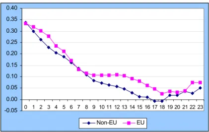
Figure 6.1.3 displays how the predicted savings from the model compare to the actual savings according to immigrants’ EU status. For non-EU immigrants, the model captures the downward-sloping profile of savings. The level of savings fit well, too. The only exceptions, again, are thefirst and last few periods where the observations are fewer. As can also be seen from thefigure, the model predicts theflat profile of the savings function of EU immigrants around 9,000DM very well. The model also captures the decline toward the last few periods. However, this decline is not as strong as it is seen in the data. Once more, this is due to the fact that the strong decline in the data is brought about by a few observations who are smoothed out by the higher frequency of observations in the middle ranges.23
The exogenous transitions whose outcomes are used in the estimation include employ-ment, retireemploy-ment, and earnings functions. Figures E.1 presents thefit of employment status according to EU status. In both cases, the predictions match the data quite well. They cap-ture the decreasing profile of the employment probability as well as the difference between the immigrants according to their EU status in their employment probability. Furthermore, the levels are very similar. The fit for retirement transition is shown in Table E.1 for all 23Note that we can not compare the saving predictions of our model in thefirst 5 periods as there is no savings information at these periods in the data. Our model predicts that both EU and non-EU immigrants save more than a third of their income right after arrival. This high saving rate is consistent with the findings of the literature as to immigrants’ savings in Germany. Paine (1974), based on a report by the State Planning Organization of Turkey in 1971 —when all Turkish guestworkers would be in Germany for less then 5 periods—, reports a saving rate of 36 percent. Based on a study conducted by the Central Bank of Turkey in 1986, which gathered saving and income information according to immigrants’ duration of residence, we find that the saving rate of Turkish immigrants with less than four years of residence was 39 percent.
immigrants. I keep this at a more aggregated level because the number of observations gets too small. Although the model overstates the percentage of retired immigrants, in particular at ages 62 and 64, it provides a good approximation to the actual transition to retirement. The prediction of the model for the income variable is presented in Figures E.2 separately for EU and non-EU immigrants. In both cases, the model predicts the level and shape of the profile well. It captures the fact that the hump is weak as well as the fact that it is weaker for non-EU immigrants. As always, the fit is worse in the beginning and ending periods where the data are sparse.
I believe that the above evidence of the model fit provide a good case for the credibility of the model. Obviously, the credibility of the implications of the model and the results of the counterfactual experiments hinges on the credibility of the model.
6.2
Parameter Estimates
The estimated parameters and their standard errors are presented in Appendix D. There are 124 parameters in the model. I am not interested in the estimated value of any parameters per se; however, here I will examine the parameters of value of returning home function —because this is the most ad hoc part of the model and I would like to check whether the estimated values are reasonable— and the estimated values of type characteristics because the differences among the types help us understand the key features of the behavior of immigrants as well as the results of counterfactuals in the following sections.
In the value of living in the home country function, estimated values of country dummies are all as expected. Non-EU countries have much lower values because of not only the less attractive economic conditions but also the insititutional differences. Within the EU group, Greece is less attractive compared to the other two and within the non-EU group Yugoslavia is less attractive. In the former case, economic conditions are more likely to be the cause while political conditions probably play a more important role in the latter case. With respect to the value of earnings in the home country after return, the estimated parameters and the age distribution at the time of return imply that 13 percent of Turkish return migrants receive some level of utility form employment earnings after return. Dustmann and Kirsckampf report, based on a sample of Turkish return migrants, that only 6 percent were salaried workers. In their study, return migrants were sampled two years after their return from Germany. Therefore, my estimate provides an upper bound to theirs and is consistent with the number they report.
I assumed that immigrants differ in terms of their unobserved permanent characteristics with respect to their psychic costs of living in Germany, bequest motive, marginal utility of consumption and labor market ability. According to the estimated parameteres Table 6.2.1 ranks the four types for each of these characteristics and Figure 6.2.1 displays the hazard function and mean savings profile for all immigrants by type.
Type 2 and type 4 immigrants can be classified as returners. They have higher psychic costs compared to the stayer types. Moreover, they have a lower bequest motive and a higher marginal utility of consumption which also increases their willingness to return and decumulate their asset holdings. While the psychic costs of type 2 immigrants do not change much over their life cycle, type 4 immigrants show a faster acclimatization to Germany. This causes the decline in the hazard function in thefirst 10 periods for type 4 immigrants. Another distinguishing feature of type 2 immigrants from type 4 immigrants is their higher savings ability due to higher labor market ability. As a result of this, more of the type 2 immigrants are middle-aged workers who return to live on their accumulated wealth in their home country. Type 4 immigrants have very high return rates after retirement because the difference between the values of staying and returning is the smallest and, therefore, the increase in the value of returning at retirement makes the biggest difference for this group.
One key feature of the saving decision by type is that while the profile is relatively
flat over time for stayers, it is downward sloping for the returner types. In fact, returner types dissave in later periods. This is especially prominent for type 2 immigrants whose higher saving ability compared to the other returner type let them accumulate more assets in earlier periods. The marginal utility of holding assets changes over time because that utility depends on the length of the remaining lifetime and after a certain age the marginal utility of dissaving assets exceeds the marginal utility of holding them for immigrants with relatively low bequest motives and high marginal utility of consumption. That is the returner types, especially type 2 immigrants, start dissaving after a certain age. Another reason to the downward-sloping profile of type 2 immigrants is the out-selection dynamics within this type. Some can save faster than others due to their higher earnings and/or lower minimum consumption needs. Those that can save the fastest also return the earliest. As the highest savers are selected out, savings of the remaining ones decrease. A comparison of the saving behavior of stayer types reveals that type 1 immigrants save more than type 3 immigrants because they have higher earnings. Besides, their bequest motive is higher.
the host country, we would expect the returners to save more than the stayers and this is what we see in Figure 6.2.1. Despite having lower income, type 2 immigrants save more than type 3 immigrants and have higher asset holdings except for toward the end of their lifetime at which time their strong decumulation motive causes a fall in their asset holdings.
Table 6.2.2 lists the proportion of each type by nationality over duration of residence. At arrival, the fraction of returner types, types 2 and 4, is higher among EU immigrants. Their share is around forty percent for ex-Yugoslavian immigrants and sixty-one percent for Turkish immigrants. This share rises to eigthy pecent for Italian immigrants, it is above eighty-five percent for Greek and above ninety percent for Spanish immigrants. Among the returner types, a higher share is type 2 among non-EU immigrants, especially so for Turkish immigrants. For Greek immigrants, type 2 and type 4 immigrants are half and half whereas Spanish and Italian immigrants have a higher share of type 4 immigrants, especially Italians. One key difference between the two returner types is their labor market ability. Type 2 immigrants have higher income. Both stayer types have even higher income. Since EU immigrants have a lower fraction of type 2 immigrants among the returners as well as a lower fraction of stayers, they have lower incomes on average at arrival. This is consistent with the
findings of literature on guest-workers. Martin (1980) reports that there was a high demand in Turkey for emigration during the recruitment scheme, which meant that German agencies could be selective.24 Paine (1974) reports a similar experience for Yugoslavia in that most
of the urban migrants belonged to the skilled elite rather than the unemployed. Therefore, there was positive selection in the immigration of guestworkers from non-EU countries. On the other hand, a higher fraction of the immigrants coming from the EU countries were villagers from poor areas of these countries.
7
IMPLICATIONS OF THE RESULTS
Here, I discuss two important implications of immigrants’ return and savings behavior. One is important from the host country’s perpective, net contributions of immigrants to the pension insurance and unemployment insurance systems, and the other is important from 24According to Martin (1980) “With 10 Turks wanting to work in Germany for each one recruited by employers, the Germans could be selective, and they were. Some 30 to 40 percent of the Turks recruited to work in Germany were skilled workers in Turkey who worked as manual laborers in Germany. By 1970, for example, 40 percent of Turkey’s carpenters and stonemasons were employed in Germany, often as assembly line or unskilled workers.”
the source countries’ perpective, how much assets immigrants bring with them when they return.
7.1
Net Pension and Unemployment Insurance Contributions
In this section, I analyze the value at arrival of immigrants’ net lifetime pension and unem-ployment insurance contributions. Figure 7.1.1 presents the net contributions to the pension and unemployment insurances separately by country of origin and age at entry.
Net contributions of non-EU immigrants to the pension insurance system are much higher. Non-EU immigrants have shorter life spans; therefore, their lifetime pension benefits are lower. In addition, higher return rates of EU immigrants in the early periods imply that they contribute for a shorter duration of time. A shorter contribution period implies that when the net contribution of each additional year of residence is positive, lifetime contributions will include a fewer number of positive net contributions and, therefore, will be lower. The net contribution from staying one more year is higher in the earlier periods, except for period three which is the qualification period. However, staying longer than that makes up for the negative contribution in period three. The contribution of each additional year is lower at later periods because immigrants are more likely to be unemployed and, therefore, making no contributions. Besides each additional year’s contribution at later periods is discounted more whereas the increase in present value of benefits caused by an additional year of residence does not depend on the total duration of residence.
As can also be seen in the figure, net contributions of younger age-at-entry groups to the pension insurance are higher. Holding income constant, older age-at-entry groups will claim lower benefits after retirement due to their shorter contribution periods; therefore, the net contribution of each additional year of residence is higher for them. On the other hand, a shorter contribution period also implies that, when the net contribution of each additional year of residence is positive, lifetime contribution will include a fewer number of positive net contributions. Moreover,.since the fraction of worklife spent as unemployed is lower for younger age-at-entry groups, their contributions are higher. The last two facts dominates the first one and as can be seen from the figure net contributions fall as age-at-entry inceases. This decline in net contributions as age-at-age-at-entry increases is faster for non-EU immigrants. This is caused by the fact that non-EU immigrants that enter at younger ages have significantly higher incomes than older age-at-entry cohorts of non-EU immigrants; whereas the income gap according to age-at-entry for EU immigrants is much smaller.
Another interesting feature of Figure 7.1.1 is that net contributions after middle age-at-entry values for Italians rise unlike those for the Greek and Spanish. For all EU groups, incomes at entry for older age-at-entry groups are higher. However, for Italian immigrants, the difference between the incomes of older age-at-entry groups and younger age-at-entry groups is bigger. In addition, the difference between the return rates of older and younger age-at-entry cohorts is bigger as well. Younger age-at-entry groups of Italian immigrants are much more likely to return, keeping their contributions at a low level.
Next, I examine the net contributions of immigrants to the unemployment insurance system. The two key features of thefigure are that immigrants from non-EU countries have much lower net contributions and that net contributions decrease as immigrants’ age at entry increases for all nationalities. Both features result from the employment transition of immigrants as shown above in Figure 4.1.1. Unemployment rates of non-EU immigrants are higher than those of EU immigrants and since all immigrants are much more likely to be unemployed at older ages, older age-at-entry cohorts spend a larger fraction of their residence in Germany as unemployed.
An interesting feature of Figure 7.1.2 is that for immigrants who enter before the age of 34, Turkish immigrants have higher net contributions than ex-Yugoslavian immigrants whereas afterwards it is vice versa. Unemployment rates of Turkish immigrants are higher regardless of age at entry. However, their return rates are also higher. Unemployment really becomes an issue at older ages and among the younger age-at-entry cohorts, a much higher fraction of Turkish immigrants return before reaching older ages compared to ex-Yugoslavian immigrants. For instance, for those who enter at the age of 18, sixty percent of the Turkish immigrants return by the age offifty whereas only thirty-five percent of the ex-Yugoslavian immigrants return by the same age. For older age-at-entry cohorts higher return rates of Turkish immigrants do not matter as much because unemployment rates immediately get higher and there is a smaller difference between the hazard rates of the two nationalities for older age-at-entry cohorts. This is another feature that emphasizes the importance of return behavior in determining the impact of immigration.
In order to get a more aggregate look at immigrants’ impact on the host country social security system, I combine the net contributions to the pension and unemployment insurance systems.25 The results are displayed in Figure 7.1.2. Younger age-at-entry cohorts make
25The only element of the social security system we are missing here is the health insurance system. Since participation in this insurance system entitles not only the immigrant himself but also his family to benefits,