University of Pennsylvania
University of Pennsylvania
ScholarlyCommons
ScholarlyCommons
Technical Reports (CIS)
Department of Computer & Information Science
1-1-2010
Inference Driven Metric Learning (IDML) for Graph Construction
Inference Driven Metric Learning (IDML) for Graph Construction
Paramveer S. Dhillon
University of Pennsylvania
Partha Pratim Talukdar
University of PennsylvaniaKoby Crammer
Technion-Israel Institute of Technology
Follow this and additional works at: https://repository.upenn.edu/cis_reports
Recommended Citation
Recommended Citation
Paramveer S. Dhillon, Partha Pratim Talukdar, and Koby Crammer, "Inference Driven Metric Learning (IDML) for Graph Construction", . January 2010.
University of Pennsylvania Department of Computer and Information Science Technical Report No. MS-CIS-10-18. This paper is posted at ScholarlyCommons. https://repository.upenn.edu/cis_reports/927
Inference Driven Metric Learning (IDML) for Graph Construction
Inference Driven Metric Learning (IDML) for Graph Construction
Abstract
Abstract
Graph-based semi-supervised learning (SSL) methods usually consist of two stages: in the first stage, a graph is constructed from the set of input instances; and in the second stage, the available label information along with the constructed graph is used to assign labels to the unlabeled instances. Most of the previously proposed graph construction methods are unsupervised in nature, as they ignore the label information already present in the SSL setting in which they operate. In this paper, we explore how available labeled instances can be used to construct a better graph which is tailored to the current classification task. To achieve this goal, we evaluate effectiveness of various supervised metric learning algorithms during graph construction. Additionally, we propose a new metric learning framework:
Inference Driven Metric Learning (IDML), which extends existing supervised metric learning algorithms to exploit widely available unlabeled data during the metric learning step itself. We provide extensive empirical evidence demonstrating that inference over graph constructed using IDML learned metric can lead to significant reduction in classification error, compared to inference over graphs constructed using existing techniques. Finally, we demonstrate how active learning can be successfully incorporated within the the IDML framework to reduce the amount of supervision necessary during graph construction.
Comments
Comments
University of Pennsylvania Department of Computer and Information Science Technical Report No. MS-CIS-10-18.
Inference Driven Metric Learning (IDML) for
Graph Construction
Paramveer S. Dhillon1, Partha Pratim Talukdar1, and Koby Crammer2 1 CIS Department, University of Pennsylvania, Philadelphia, PA 19104, U.S.A.
2 Electrical Engineering Department, The Technion, Haifa 32000, Israel.
Abstract. Graph-based semi-supervised learning (SSL) methods usu-ally consist of two stages: in the first stage, a graph is constructed from the set of input instances; and in the second stage, the available label information along with the constructed graph is used to assign labels to the unlabeled instances.
Most of the previously proposed graph construction methods are unsu-pervised in nature, as they ignore the label information already present in the SSL setting in which they operate. In this paper, we explore how available labeled instances can be used to construct a better graph which is tailored to the current classification task. To achieve this goal, we eval-uate effectiveness of varioussupervised metric learning algorithms dur-ing graph construction. Additionally, we propose a new metric learndur-ing framework: Inference Driven Metric Learning (IDML), which extends existing supervised metric learning algorithms to exploit widely avail-able unlabeled data during the metric learning step itself. We provide extensive empirical evidence demonstrating that inference over graph constructed using IDML learned metric can lead to significant reduction in classification error, compared to inference over graphs constructed us-ing existus-ing techniques. Finally, we demonstrate how active learnus-ing can be successfully incorporated within the the IDML framework to reduce the amount of supervision necessary during graph construction.
1
Introduction
Supervised machine learning algorithms have been quite successful in a vari-ety of domains, ranging from Natural Language Processing to Bioinformatics. Unfortunately, such algorithms require large amounts of labeled data which is expensive and time consuming to prepare. To addresses this issue, recent re-search has focused on Semi-Supervised Learning (SSL) algorithms, which learn from limited amounts of labeled data combined with widely available unlabeled data. In particular, graph based SSL algorithms have recently been successfully used in different tasks, e.g. the work of [1].
Given a set of instances, some of which are labeled while the rest are un-labeled, most graph based SSL algorithms first construct a graph where each node corresponds to an instance. Similar nodes are connected by an edge, with edge weight encoding the degree of similarity. Once the graph is constructed, the
nodes corresponding to labeled instances are injected with the corresponding la-bel. Using this initial label information along with the graph structure, graph based SSL algorithms assign labels to all unlabeled nodes in the graph. Most of the graph based SSL algorithms are iterative and also parallelizable, making them suitable for SSL setting where vast amounts of unlabeled data is usu-ally available. Examples of a few graph-based SSL algorithms include Gaussian Random Fields (GRF) [2], Local and Global Consistency (LGC) [3], Manifold Regularization (MR) [4], Quadratic Criteria (QR) [5], Graph Transduction via Alternating Minimization (GTAM) [6], Adsorption and its variants [7], Measure Propagation [8].
Most of the graph based SSL algorithms mentioned above concentrate pri-marily on the label inference part, i.e. assigning labels to nodes once the graph has already been constructed, with very little emphasis on construction of the graph itself. Only recently, the issue of graph construction has begun to receive attention [9–11]. Ab-matching (BM) based method for regular graph construc-tion is presented by [10], where each node in the constructed graph is required to have the same degree (b). [11] proposed that each node is required to have a minimum weighted degree of 1, which is relaxed in some cases. Both of these methods emphasize on constructing graphs which satisfy certain structural prop-erties (e.g. degree constraints on each node). Since our focus is on SSL, a certain number of labeled instances are available at our disposal. However, the graph construction methods mentioned above are all unsupervised in nature, i.e. they do not utilize available label information during the graph construction process. In fact, this is left as an open question for future work in [11]. In this paper, we propose a fill to gap and explore how the available label information can be used for graph construction in graph based SSL. In particular, we focus on learning
a distance metric using available label information, which can then be used to set the edge weights on the constructed graph.
Once the nodes in a graph are fixed, the rest of graph construction pro-cess reduces to setting the edge weights on a complete graph, with an edge weight of 0 encoding absence of the corresponding edge. Over the years, several
supervised metric learning algorithms have been developed, with Information-theoretic Metric Learning (ITML) [12] and large margin distance metric learning (LMNN) [13] being two recent and state-of-the-art metric learning methods. The distance metric learned by such methods can be used to compute similarity3
be-tween a pair of instances, and subsequently set as the similarity edge weight on the edge connecting the instances in the graph.
In this paper, we make the following contributions:
1. In contrast to previously proposed unsupervised graph construction meth-ods which ignore already available label information, we empirically validate effectiveness ofsupervised distance metric learning algorithms during graph construction for graph based SSL.
3 By using an appropriate distance to similarity mapping, e.g. Gaussian kernel which
2. In order to exploit widely available unlabeled data during distance met-ric learning, we propose a new metmet-ric learning framework: Inference Driven Metric Learning (IDML). We provide extensive empirical evidence demon-strating that inference over graph constructed using IDML learned metric can lead to significant reduction in classification error, compared to inference over graphs constructed using existing techniques.
3. Finally, we demonstrate how active learning can be incorporated within the IDML framework to reduce the amount of supervision necessary dur-ing graph construction.
The paper is organized as follows: in Section 3, we review two recently pro-posed metric learning algorithms, ITML and LMNN; in Section 4, we present the Inference-Driven Metric Learning (IDML) framework; in Section 5, we show how learned distance metrics can be used to construct graphs, and subsequently per-form label inference on such graphs; in Section 6, we report experimental results on various real-world datasets; and finally in Section 7, we present concluding remarks with directions for future work.
2
Notations
Let X be the d×n matrix of n instances in a d-dimensional space. Out of the ninstances, nl instances are labeled, while the remaining nu instances are unlabeled, with n= nl+nu. G = (V, E, W) is the graph we are interested in constructing; where V is the set of vertices with|V|=n, E is the set of edges, andW is the symmetricn×nmatrix of edge weights that we would like to learn.
Wij is the weight of edge (i, j), and also the similarity between instancesxi and
xj.S is an×ndiagonal matrix with Sii= 1 iff instancexi is labeled.mis the total number of labels.Y is then×mmatrix storing training label information, if any. ˆY is the n×mmatrix of estimated label information, i.e. output of any inference algorithm (e.g. see Section 5). A is a positive definite matrix of size
d×d, which parametrizes the (squared) Mahalanobis distance (Equation 1).
3
Metric Learning Review
We now review some of the recently proposedsupervised methods for learning Mahalanobis distance between instance pairs. We shall concentrate on learning matrixAwhich parametrizes the distance,dA(xi, xj), between instancesxi and
xj.
dA(xi, xj) = (xi−xj)A(xi−xj) (1) SinceA is positive definite, we can decompose it as A=PP, whereP is another matrix of sized×d. We can then rewrite Equation 1 as,
dA(xi, xj) = (xi−xj)PP(xi−xj) = (P xi−P xj)(P xi−P xj)
Hence, computing Mahalanobis distance w.r.t.Ais equivalent to first project-ing the instances into a new space usproject-ing an appropriate transformation matrix
P and then computing Euclidean distance in the linearly transformed space.
3.1 Information-Theoretic Metric Learning (ITML)
Information-Theoretic Metric Learning (ITML) [12] assumes the availability of prior knowledge about inter-instance distances. In this scheme, two instances are considered similar if the Mahalanobis distance between them is upper bounded, i.e.dA(xi, xj)≤u, whereuis a non-trivial upper bound. Similarly, two instances are considered dissimilar if the distance between them is larger than certain thresholdl, i.e.dA(xi, xj)≥l. Similar instances are represented by setS, while dissimilar instances are represented by setD.
In addition to prior knowledge about inter-instance distances, sometimes prior information about the matrixA, denoted byA0, itself may also be available.
For example, Euclidean distance (i.e.A0=I) may work well in some domains.
In such cases, we would like the learned matrix Ato be as close as possible to the prior matrix A0. ITML combines these two types of prior information, i.e.
knowledge about inter-instance distances, and prior matrixA0, in order to learn
the matrixA by solving the optimization problem shown in (3). min
A0 Dld(A, A0) (3)
s.t. tr{A(xi−xj)(xi−xj)} ≤u, ∀(i, j)∈S
tr{A(xi−xj)(xi−xj)} ≥l, ∀(i, j)∈D
whereDld(A, A0) = tr(AA−01)−log det(AA− 1
0 )−n, is the LogDet divergence.
It may not always be possible to exactly solve the optimization problem shown in (3). To handle such situations, slack variables may be introduced to the ITML objective. Following the notation in [12], letc(i, j) be the index of the (i, j)thconstraint, and letξbe a vector of length|S|+|D|of slack variables.ξis
initialized to ξ0, whose components equalufor similarity constraints, andl for
dissimilarity constraints. The modified ITML objective involving slack variables is shown in (4).
min
A0,ξ Dld(A, A0) +γ·Dld(ξ, ξ0) (4)
s.t. tr{A(xi−xj)(xi−xj)} ≤ξc(i,j), ∀(i, j)∈S
tr{A(xi−xj)(xi−xj)} ≥ξc(i,j), ∀(i, j)∈D
where γ is a hyperparameter which determines the importance of violated constraints. To solve the optimization problem in (4), an algorithm involving repeated Bregman projections is presented in [12], which we use for the experi-ments reported in this paper.
3.2 Large Margin Nearest Neighbor (LMNN)
A large margin based method for learning a Mahalanobis distance metric from labeled instances is presented in [13]. The objective here is to learn a linear
transformation of input instances so that thek nearest neighbors (in the linearly transformed space) of each instance share the same label. This metric learning algorithm is tuned towards achieving good performance on k-NN classification. From now on, we shall refer to this large margin metric learning algorithm in [13] as LMNN.
A set of labeled instances and a hyperparameterkis input to LMNN. For each labeled instance, LMNN first determines ktarget neighbors. Target neighbors of an instance xi are the instances that LMNN desires to be closest to xi in the linearly transformed target space. The target neighbors are fixed at the start of the algorithm and are not changed subsequently. In many domains, the target neighbors may be selected based on prior knowledge. Another alternative is to select the target neighbors based on Euclidean neighbors in the original space, which is the strategy we use for the experiments in this paper (as in [13]).
Once the target neighbors for each instance is determined, LMNN learns a linear transformation so that for each point, the closest point from a different class (called impostor) is further away by a margin from the farthest target neighbor of the point, with all distances measured in the linearly transformed space. In other words, an instance’s target neighbors define a neighborhood where instances from other classes are not allowed. In order to achieve this goal, LMNN solves a convex optimization problem which is reproduced from [13] in (5).
min A,ξ (1−μ) i,j∈N(i) dA(xi, xj) + μ i,j∈N(i),l (1−yil)ξijl (5)
s.t. dA(xi, xl)−dA(xi, xj)≥1−ξijl (6)
A0, ξijl≥0
wheredAis the Mahalanobis distance w.r.t A as shown in Equation 1,N(i) consists of xi’s target neighbors, {yil} are indicator variables with yil = 1 iff
yi = yl, {ξijl} are slack variables which allow violation of the large margin constraint (6), but with a cost whose contribution to the objective is controlled by the hyperparameterμ. The large margin constraint (6) enforces the requirement that an impostor, xl (impostors are indexed byl), should be at asafe distance away fromxi. The first term in (5) represents the fact that LMNN tries to pull
together all instances within a target neighborhood. As noted by [13], as most input instance pairs,xi andxl, are likely to be well separated from each other, most of the slack variables{ξijl}are never going to get assigned positive values. This sparseness property can be exploited to develop faster, special purpose solver to optimize the LMNN objective shown above [13].
After optimizing the LMNN objective, we obtain a positive semi-definite matrixAwhich can be used to compute the Mahalanobis distance between any two instances using Equation 1.
Algorithm 1Inference Driven Metric Learning (IDML)
Input: instances X, training labelsY, training instance indicator S, label en-tropy thresholdβ, neighborhood sizek
Output: Mahalanobis distance parameterA
1: ˆY ←Y, ˆS←S 2: repeat 3: A←MetricLearner(X,S,ˆ Yˆ) 4: W ←ConstructKnnGraph(X, A, k) 5: Yˆ←GraphLabelInference(W,S,ˆ Yˆ) 6: U ←SelectLowEntInstances( ˆY,S, βˆ ) 7: Yˆ←Yˆ+UYˆ 8: Sˆ←Sˆ+U
9: untilconvergence (i.e.Uii= 0, ∀i) 10: return A
4
Inference Driven Metric Learning (IDML)
The metric learning algorithms we have reviewed so far, ITML in Section 3.1 and LMNN in Section 3.2, are supervised in nature, and hence they do not exploit widely available unlabeled data. In this section, we present Inference Driven Metric Learning (IDML) (Algorithm 1), a metric learning framework which combines existing supervised metric learning algorithm (such as ITML or LMNN) along with trasnductive graph-based label inference to learn a new distance metric from labeled as well as unlabeled data combined. In self-training styled iterations, IDML alternates between metric learning and label inference; with output of label inference used during next round of metric learning, and so on.
IDML starts out with the assumption that existing supervised metric learning algorithms, such as ITML and LMNN, can learn a better metric if the number of available labeled instances is increased. Since we are focusing in the SSL setting with nl labeled and nu unlabeled instances, the idea is to automatically label the unlabeled instances using a graph based SSL algorithm, and then include instances with low assigned label entropy (i.e. high confidence label assignments) in the next round of metric learning. The number of instances added in each iteration depends on the threshold β4. This process is continued until no new
instances can be added to the set of labeled instances, which can happen when either all the instances are already exhausted, or when none of the remaining unlabeled instances can be assigned labels with high confidence.
The IDML framework is presented in Algorithm 1. In Line 1, any supervised metric learner, such as ITML or LMNN, may be used as theMetricLearner. Using the distance metric learned in Line 1, a new k-NN graph is constructed in
4 During the experiments in Section 6, we set β = 0.05 and observed that the low
entropy instances, which are selected for inclusion in next iteration of metric learning, are usually classified with fairly high accuracy.
Line 1, whose edge weight matrix is stored inW. In Line 1,GraphLabelInference optimizes over the newly constructed graph the GRF objective [2] shown in (7).
min
ˆ
Y
tr{YˆLYˆ}, s.t. SˆYˆ = ˆSYˆ (7) whereL=D−Wis the (unnormalized) Laplacian, andDis a diagonal matrix with Dii =jWij. The constraint, ˆSYˆ = ˆSYˆ, in (7) makes sure that labels on training instances are not changed during inference. In Line 1, a currently unlabeled instancexi(i.e. ˆSii= 0) is considered a new labeled training instance, i.e.Uii = 1, for next round of metric learning if the instance has been assigned labels with high confidence in the current iteration, i.e. if its label distribution has low entropy (i.e. Entropy( ˆYi:) ≤ β). Finally in Line 1, training instance
label information is updated. This iterative process is continued till no new labeled instance can be added, i.e. whenUii = 0∀i. IDML returns the learned matrixA which can be used to compute Mahalanobis distance using Equation 1.
Lemma: IDML (Algorithm 1) will terminate after at mostniterations.
Proof: The GraphLabelInference method used in IDML ensures that
labels of already labeled instances are not changed (see (7)). Hence, once an instance is assigned a label in one of the iterations (Line 1), its label is not changed in all subsequent iterations. Since there are only finitely many points, hence only a finite number of new points can be selected in Line 1 of IDML. Hence, IDML can iterate for at most niterations, where nis the total number of instances.
4.1 Relationship to Other Methods
IDML is similar in spirit to the EM-based HMRF-KMeans algorithm in [14], which focuses on integrating constraints and metric learning for semi-supervised clustering. However, there are crucial differences. Firstly, the inference algorithm in [14] is parametric (k-Means), while the inference in IDML is non-parametric (graph based). Secondly, and more importantly, the label constraints in [14] are hard constraints which are fixed a-priori and are not changed during EM iterations. In case of IDML , the graph structure induced in each iteration (Line 1 in Algorithm 1) imposes a Manifold Regularization (MR) [4] style smoothing penalty, as shown in (7). Hence, compared to the hard and fixed constraints in HMRF-KMeans, IDML constraints are soft and new constraints are added in each iteration of the algorithm.
The main difference that separates IDML from previous work on supervised metric learning [12, 13, 15] is the use of unlabeled data during metric learning. Moreover, in all of these previously proposed algorithms, the constraints used during metric learning are fixed a-priori, as they are usually derived from la-beled instances which don’t change during the course of algorithm; while the constraints in IDML are adaptive and new constraints are added in each itera-tion, when automatically labeled instances are included in each iteration (Line
1). In Section 6, we shall see experimental evidence that these additional con-straints can be quite effective in improving IDML’s performance compared to ITML or LMNN.
The distance metric learned using IDML can be used to compute inter-instance distance in b-matching (BM) [10], and in this way the two approaches can compliment one another.
5
Graph Construction & Inference
Gaussian kernel [2, 16], a widely used measure of similarity between data in-stances, can be used to compute edge weights as shown in Equation 8.
Wij = exp −dA(xi, xj) 2σ2 (8) where dA(xi, xj) is the distance measure between instances xi and xj, and
σ is the kernel bandwidth parameter. By setting A = I, we get the standard Euclidean distance in input space, which has traditionally been used in previous work [2]. Instead, by usingAas learned by metric learning algorithms in Section 3.1, 3.2 or 4, we can define a similarity metric which is tailored to the current classification task.
Setting edge weights directly using Equation 8 will result in a complete graph, where any two pair of nodes will be connected with a positively weighted edge. This may be undesirable as a dense graph may slow down any subsequent infer-ence. We may sparsify the graph by retaining only edges toknearest neighbors of each node, and dropping all other edges (i.e. setting corresponding edge weights to 0), a commonly used graph sparsification strategy. As an alternative, other recently proposed method (e.g.b-matching [10]) may also be used to generate a sparse graph.
Inference: With the graphG= (V, E, W) constructed, we may now perform inference over this graph to assign labels to allnu unlabeled nodes. Any of the several graph based SSL algorithms mentioned in Section 1 may be used for this task. For the experiments in this paper, we use the GRF algorithm [2] which minimizes the optimization problem shown in (7).
6
Experiments
In this section, we evaluate the importance of metric learning for constructing graphs, where the constructed graphs, along with the labeled instances, are used to classify initially unlabeled instances. We evaluate performance using classifica-tion error (i.e. 1 - accuracy) . We use Gaussian kernel to set edge weights, followed by k-NN graph sparsification, as described in Section 5. The hyperparameters
k ∈ {2,5,10,50,100,200,500,1000} and the Gaussian kernel bandwidth mul-tiplier5,
ρ ∈ {1,2,5,10,50,100}, are tuned on a separate development set. In
5 σ=ρ σ
Dataset Type Dimension Balanced Amazon Real-World 132553 Yes Newsgroups Real-World 32965 Yes Reuters Real-World 10964 Yes EnronA Real-World 5802 No Text Real-World 11960 Yes USPS Real-World 241 No BCI Real-World 117 Yes Digit Artificial 241 No
Table 1. Description of datasets used in experiments in Section 6. All datasets were binary, with 1500 total instances in each, except BCI which had 400 instances.
all experiments, GRF (see Section 5) is used. Similarly, we use standard im-plementations of ITML and LMNN made available by respective authors. Brief description of the datasets used for experiments in this section is presented in Table 1; the first four datasets are obtained from [17], while the rest are from [18].
6.1 Results on Real-World Datasets
Datasets Original RP PCA ITML LMNN IDML-LM IDML-IT Amazon 0.4686 0.4681 0.2329 0.1542 0.2069 0.2065 0.1537 Newsgroups 0.3648 0.3778 0.3490 0.1791 0.2860 0.2791 0.1650 Reuters 0.2912 0.5016 0.5016 0.1300 0.4991 0.4003 0.1264 EnronA 0.3514 0.3514 0.3200 0.1855 0.3124 0.3096 0.1671 Text 0.4541 0.4954 0.4835 0.3140 0.3297 0.3247 0.3121 USPS 0.1536 0.1667 – 0.1484 0.1388 0.1388 0.1467 BCI 0.4693 0.4678 – 0.4264 0.4122 0.4093 0.4196 Digit 0.0246 0.0357 – 0.0438 0.1186 0.0991 0.0381
Table 2. Comparison of transductive classification performance over graphs con-structed using different methods (see Section 6.1), with nl = 50 and nu = 1450. All results are averaged over four trials. IDML-LM and IDML-IT are the proposed methods.
In this section, we compare the following methods of estimatingA, which in turn is used in Equation 8 to estimate edge weights:
Original: We setA=Id×d, i.e. the data is not transformed and Euclidean
distance in the input space is used to compute distance between instances.
RP: The data is first projected into a lower dimensional space of dimension
d = 2loglogn1
using the Random Projection (RP) method [19]. We set A =
RR, whereRis the projection matrix used by RP.was set to 0.25 for the experiments in Section 6.1.
Datasets Original RP PCA ITML LMNN IDML-LM IDML-IT Amazon 0.4046 0.3964 0.1554 0.1418 0.2405 0.2004 0.1265 Newsgroups 0.3407 0.3871 0.30980.1664 0.2172 0.2136 0.1664 Reuters 0.2928 0.3529 0.2236 0.1088 0.3093 0.2731 0.0999 EnronA 0.3246 0.3493 0.2691 0.2307 0.1852 0.1707 0.2179 Text 0.4523 0.4920 0.4820 0.3072 0.3125 0.3125 0.2893 USPS 0.0639 0.0829 – 0.1096 0.1336 0.1225 0.0834 BCI 0.4508 0.4692 – 0.4217 0.3058 0.2967 0.4081 Digit 0.0218 0.0250 – 0.0281 0.1186 0.0877 0.0281
Table 3. Comparison of transductive classification performance over graphs con-structed using different methods (see Section 6.1), with nl = 100 and nu = 1400. All results are averaged over four trials. IDML-LM and IDML-IT are the proposed methods.
PCA: Instances are first projected into a lower dimensional space using Principal Components Analysis (PCA) . For all experiments, dimensionality of the projected space was set at 2506. We set A = PP, where P is the projection matrix generated by PCA.
LMNN: A is learned by applying LMNN (see Section 3.2) on the PCA projected space (above).
ITML:A is learned by applying ITML (see Section 3.1) on the PCA pro-jected space (above).
IDML-LM: A is learned by applying IDML (Algorithm 1) on the PCA projected space (above); with LMNN used asMetricLearnerin IDML.
IDML-IT:Ais learned by applying IDML (Algorithm 1) (see Section 4) on the PCA projected space (above); with ITML used asMetricLearnerin IDML.
Experimental results on datasets in Table 1 with 50 and 100 labeled instances (nl) are shown in Tables 2 and 3, respectively. From these we observe that, con-structing a graph using a learned metric can significantly improve performance (in 13 out of 16 cases). We consistently find graphs constructed using IDML-IT to be the most effective. This is particularly true in case of high-dimensional datasets where distances in the original input space are often unreliable because of curse of dimensionality.
We tried our best to include comparisons with graphs constructed usingb -matching [10], however that often resulted in disconnected graphs which the GRF code we used (obtained from [2]) was unable to handle.
6.2 Sensitivity to Noisy Features
In order to evaluate sensitivity of IDML-IT, the best performing method from Section 6.1, to input data noise and increasing dimensions, we generated four
6 PCA was not performed on USPS, BCI and Digit as they already had dimension
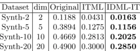
Dataset dim Original ITML IDML-IT Synth-2 2 0.1188 0.0431 0.0163 Synth-5 5 0.3894 0.1275 0.1156 Synth-10 10 0.4669 0.2813 0.2025 Synth-20 20 0.4900 0.3000 0.2850
Table 4.Results on synthetic datasets (see Section 6.2) withnl= 100. All results are averaged over four trials.
synthetic datasets: Synth-{2,5,10,20}, each consisting of 500 instances in Rd
(d= 2,5,10,20, respectively), where the first two dimensions were sampled from a 45orotated Gaussian distribution with standard deviation 1. The remainingd−
2 dimensions were sampled independently from Gaussian distributionsN(0,2). Hence, in these datasets, only the first two dimensions are informative, while the rest of the dimensions just add noise.
Experimental results on these synthetic datasets with 100 labeled instances are presented in Table 4. From Table 4, we observe that label inference over graphs constructed using IDML-IT achieve lowest classification error across all datasets. We also observe that as the number of noisy dimensions were increased (from 0 in Synth-2 to 18 in Synth-20), performance in case of Original deterio-rated significantly, while IDML-IT is much more resilient to noise. This demon-strates the fact that the learned distance metric is able to filter out the noisy dimensions and concentrate more on the first two informative dimensions, which is essential in these datasets. It is interesting to note that IDML-IT is very effective even in the absence of noise (Synth-2).
6.3 Active Learning 25 50 75 100 125 0.1 0.2 0.3 0.4 0.5
Number of Labeled Instances
Classification Error Amazon Dataset Random−Active IDML−IT−Active 25 50 75 100 125 0.2 0.25 0.3 0.35 0.4
Number of Labeled Instances
Classification Error
EnronA Dataset Random−Active IDML−IT−Active
Fig. 1.Results from active learning experiments in Section 6.3. All results are averaged over four trials. Active learning using IDML-IT-Active is the bottom line.
In all the experiments reported so far in Sections 6.1 and 6.2, thenltraining instances, usually labeled by humans, are fixed at the start and are not changed during course of the algorithms. In case of IDML-LM and IDML-IT, this initial set of labeled instances is augmented by addingautomatically labeled instances with low label entropy (Line 1 in Algorithm 1).
In this section, we take an active learning view and explore whether the in-stances to be labeled (by a human or an oracle) can be actively selected using a modified version of IDML-IT, which we call IDML-IT-Active. Instead of adding instances with low label entropy as in IDML-IT; IDML-IT-Active selects, at each iteration, top-rinstances with highest label entropy which are then labeled by a human or an oracle. These additionalroracle labeled (as opposed toautomatic
labeling in IDML-IT) instances are used in the next iteration of metric learning. In Figure 1, we compare label inference over graphs constructed using IDML-IT-Active, to graphs constructed in the original space (i.e. A=I) with equivalent number of randomly selected and labeled instances, called Random-Active in Figure 1. Across both the datasets, we observe that 25-50 actively selected in-stances using IDML-IT-Active performs better than 125 randomly selected and labeled instances, thereby drastically reducing the amount of supervision neces-sary to attain a certain level of classification performance.
7
Conclusion
In this paper, we explored how labeled instances, available in the SSL setting, can be used to construct a better graph for improved classification accuracy in graph based SSL. We demonstrated effectiveness of various supervised met-ric learning algorithms to learn distance metmet-rics for graph construction, and subsequent inference over such constructed graphs. To the best of our knowl-edge, this is the first study of its kind where effectiveness of metric learning for graph construction is studied. Additionally, we proposed a new metric learning framework: Inference Driven Metric Learning (IDML), which extends existing supervised metric learning algorithms to exploit widely available unlabeled data during the metric learning step itself. Through a set of extensive experiments on synthetic as well as various real-world datasets, we demonstrated that infer-ence over graphs constructed using IDML can lead to significant reduction in classification error, compared to inference over graphs constructed either with a supervised metric learner in isolation, or without using any label information at all. Finally, we demonstrated how labeled instances can be actively selected within the the IDML framework to reduce the amount of supervision necessary during graph construction.
Encouraged by these promising initial results, we plan to investigate further into the Inference Driven Metric Learning (IDML) framework, and in particular pose it as an optimization of a regularized metric learning objective.
References
1. Subramanya, A., Bilmes, J.A.: The semi-supervised switchboard transcription project. In: INTERSPEECH, Brighton, UK (September 2009)
2. Zhu, X., Ghahramani, Z., Lafferty, J.: Semi-supervised learning using Gaussian fields and harmonic functions. In: ICML. (2003)
3. Zhou, D., Bousquet, O., Lal, T., Weston, J., Schlkopf, B.: Learning with local and global consistency. In: NIPS, The MIT Press (2004)
4. Belkin, M., Niyogi, P., Sindhwani, V.: Manifold regularization: A geometric frame-work for learning from labeled and unlabeled examples. The Journal of Machine Learning Research7(2006) 2434
5. Bengio, Y., Delalleau, O., Le Roux, N.: Label propagation and quadratic criterion. Semi-supervised learning (2006) 193–216
6. Wang, J., Jebara, T., Chang, S.: Graph transduction via alternating minimization. In: ICML. (2008)
7. Talukdar, P., Crammer, K.: New Regularized Algorithms for Transductive Learn-ing. In: ECML-PKDD, Springer (2009)
8. Subramanya, A., Bilmes, J.A.: Entropic graph regularization in non-parametric semi-supervised classification. In: NIPS, Vancouver, Canada (December 2009) 9. Wang, F., Zhang, C.: Label propagation through linear neighborhoods. In: ICML.
(2006)
10. Jebara, T., Wang, J., Chang, S.: Graph construction and b-matching for semi-supervised learning. In: ICML. (2009)
11. Daitch, S., Kelner, J., Spielman, D.: Fitting a graph to vector data. In: ICML. (2009)
12. Davis, J., Kulis, B., Jain, P., Sra, S., Dhillon, I.: Information-theoretic metric learning. In: ICML. (2007)
13. Weinberger, K., Saul, L.: Distance metric learning for large margin nearest neigh-bor classification. The Journal of Machine Learning Research (2009)
14. Bilenko, M., Basu, S., Mooney, R.: Integrating constraints and metric learning in semi-supervised clustering. In: ICML. (2004)
15. Jin, R., Wang, S., Zhou, Y.: Regularized Distance Metric Learning: Theory and Algorithm. In: NIPS. (2009)
16. Belkin, M., Niyogi, P.: Towards a theoretical foundation for Laplacian-based man-ifold methods. Journal of Computer and System Sciences74(8) (2008) 1289–1308 17. Crammer, K., Dredze, M., Kulesza, A.: Multi-Class Confidence Weighted
Algo-rithms. (2009)
18. Chapelle, O., Scholkopf, B., Zien, A.: Semi-supervised learning. MIT Press (2006) 19. Bingham, E., Mannila, H.: Random projection in dimensionality reduction: