Optimal predictive kernel regression via feature space principle components

Rochester Institute of Technology

RIT Scholar Works

Articles

2011

Optimal predictive kernel regression via feature

space principle components

Ernest Fokoue

Follow this and additional works at:http://scholarworks.rit.edu/article

This Article is brought to you for free and open access by RIT Scholar Works. It has been accepted for inclusion in Articles by an authorized administrator of RIT Scholar Works. For more information, please [email protected].

Recommended Citation

Fokoue, Ernest, "Optimal predictive kernel regression via feature space principle components" (2011). p. 87-108. Accessed from http://scholarworks.rit.edu/article/133

Optimal Predictive Kernel Regression via

Feature Space Principal Components

Ernest Fokou´

e

Center for Quality and Applied Statistics, Rochester Institute of Technology

98 Lomb Memorial Drive, Rochester, NY 14623, USA

eMail:

[email protected]

Abstract

We propose a simple use of principal component analysis in feature space that allows the derivation of optimal predictive kernel regression. The proposed approach is shown to perform well on both artificial and real data. Despite its incredible simplicity, the proposed method is found to compete very well with sophisticated statistical approaches like the Relevance Vector Machine and the Support Vector Machine.

Keywords: Kernel Regression, Sparsity, Principal Component Analysis.

1

Introduction

We are given a training set _D = _{(xi,yi), i = 1,· · · , n : xi ∈ X ⊂ IRp,yi ∈ IR} where yi are

realizations of Y_i = f∗

(x_i) +_i, and _i is the noise term. For simplicity and without loss of

generality, we shall assume throughout this paper that the data are standardized. We assume

that the true function f∗

can be approximated by f_n(x) = n X j=1 wjK(x,xj), (1)

where _K:_{X × X →}IRis the Gaussian radial basis function kernel defined by

K(x_i,x_j) = exp −kxi−xjk 2 2ω2 , (2)

for some bandwidth ω >0. Now, the function f_n as defined in Eq. (1) is called a radial basis

function (RBF) with weights w1,w2,· · · ,wnand centers x1,x2,· · · ,xn, assumed to be pairwise

distinct. We shall consider _HK, the family of radial basis functions (RBF) generated by _K, i.e.

HK= ( h:IRp _→IR: _∀x_∈IRp, h(x) = k X i=1 wiK(x, ξi) :k ∈N, ξi ∈IRp,wi ∈IR )

The great appeal of_HK resides in the fact that, for any given continuous functionf, there exist

(a) a kernel _K(_·,_·), (b) an optimum number of basis functions k, (c) a set of weights _{wi}ki=1

and (d) a set of centers _{ξ_i}k

i=1 such that the corresponding function hk ∈ HK approximates f

to any desired precision. This approach to regression really became popular after the invention and publication by [1] of the Relevance Vector Machine (RVM). [7] provides one of the earliest and most comprehensive coverage of kernel methods as used in machine learning. However, it is important to note that kernel methods - as they are called in the machine learning community - owe the vast popularity partly to a strong theoretical justification by Kimerdolf and Wahba (1971)’s representer theorem. The reader is referred to [11] for a more detailed account of the above fundamental result. Kernel methods have come under intense and careful scrutiny in recent years. Researchers - probably fueled by the guarantee provided by such important results as the representer theorem - continually dig deeper into the framework, exploring a variety of aspects of it. One of the most important aspects of kernel regression - besides the crucial issue of the choice of the kernel - is the search for a sparse representation. Indeed, sparsity was the professed motivation of [1], and later of [3], [2]. In fact, for most situations and indeed most

kernels, the statistical estimation of the weights wj’s by traditional error minimization (least

squares) or density maximization (MLE) methods turns out to be an ill-posed problem, for which there is no hope of a decent solution without some form of regularization or constraints to help stabilize the solution. Of course, regularization in and of itself does not necessarily yield a sparse solution. Indeed, the form of the regularizer and/or appropriate subsequent refinements performed on the regularized solution are the keys to obtaining the desired level of sparsity.

Definition 1 Given a vector w>

= (w1,· · · ,wn) ∈IRn, we define supp(w) = {j : wj 6= 0},

and the zero-norm of w will simply be

kw_k0 =|supp(w)|=number of nonzeroes entries in w

Definition 2 Let s _∈ N be a natural number. We shall say that a solution w∗

is s-sparse if

kw∗

k0 ≤s, i.e. if w∗ has at most s nonzero entries.

Throughout this paper, we make the usual assumption that the noise terms are independent

zero-mean Gaussian random variables with the same variance σ2, i.e. _i iid_∼ N₍₀, σ2). As a

result, we have the likelihood

p(y_|w, σ2) =N_n(y_|Kw, σ2In), (3)

corresponding to the model of equation (1) conveniently rewritten in vector-matrix form as

y=Kw+, (4)

wherey= (y1,y2,· · · ,yn)T, w= (w1,w2,· · · ,wn)T, = (₁, ₂,· · · , _n)T and K= (K_ij) where

Kij =φ(kxi−xjk), i, j = 1,· · · , n. We ideally seeks to solve

min ˜

w∈IRnkw˜k0 subject to ky−Kw˜k

2 _{< η}

1.1

Main result

We consider obtaining a least squares solution to the estimation of the weight vector w.

How-ever, it turns out that

ˆ

wols= (K

>

K)−1K>y

cannot be obtained in practice, because the matrix (K>K) is typically ill-conditioned. Various

authors have restored to techniques of regularization such Ridge Regression [8] and LASSO [9] to isolate a unique solution. A typical ridge regression solution would be of the form

ˆ

wridge= (K

>

K+λI)−1_K>

y

where the ridge constant (tuning parameter) can be estimated through cross validation or generalized cross validation. It turns out that the ridge regression approach in this context is

fraught with various difficulties due to the nature of the matrix K.

1.2

Our approach

In this paper, however, we consider a straightforward technique based on the spectral

decom-position of (K>

K), namely

K>K=PΛP>.

• We use Λ to determine q, the number of relevant rows to retain inP and then form the

relevant projection matrix Q_∈Rn×q _{made up of the firstq columns ofP.}

• We then form the new n_×q relevant ”design” matrix

Z=KQ

• Then we get the q-dimensional estimate ˆwpck of the relevant weights

ˆ

wpck = (Z

>

Z)−1Z>y

• For each new vectorxnew, we first compute

anew = (K(xnew,xj),K(xnew,x2),· · · ,K(xnew,xn))

>

,

then we crucially form the q-dimensional relevant version of anew as

znew =Q

>

anew

• The point estimate of the response at xnew is then given by

ˆ

ynew =z

>

The immediate gain here lies in the fact that we use only standard spectral decomposition elements, and not complex computation is involved. We are therefore in the presence of a computationally efficient approach to prediction in kernel regression.

An even bigger benefit comes from the fact our initial computational results on both artificial and real life data show that our straightforward and intuitively simple technique works very well, and even outperforms sophisticated techniques like the relevance vector machine and the support vector machine.

R_m(f) = 1

m

X

(x

new,ynew)∈Test

(ynew−f(xnew)2

which the empirical version of

R(f) =E_{[(Y −f(X))}2_{] =}

Z

(x new,ynew)

(ynew−f(xnew)2dP(xnew,ynew)

2

Numerical explorations

2.1

First artificial example

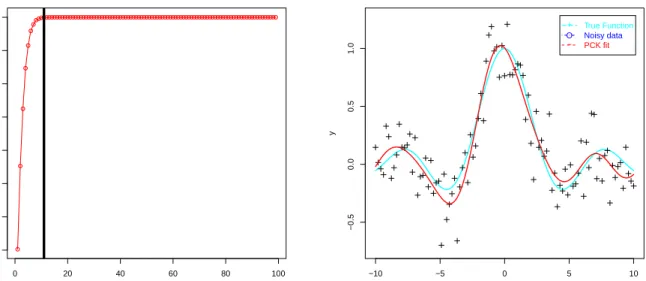
As our first illustrative example, we consider recovering the univariate sinc function from noisy observations. The choice of the sinc function is motivated by the fact that it has become the

de facto benchmark example in nearly all papers on kernel regression since its use by Vladimir Vapnik in some of the earliest computational examples of statistical learning theory.

f(x) = sin x

x x ∈[−10,+10]

We generaten = 99 points with noise varianceσ2 = 0.32_.

PCK SVM RVM

Training Error 0.0297 0.0300 0.0307 Test Error 0.2036 0.2145 0.2093

0 20 40 60 80 100 0.3 0.4 0.5 0.6 0.7 0.8 0.9 1.0 number of components Propor tion of v ar iation captured −10 −5 0 5 10 −0.5 0.0 0.5 1.0 x y + O − True Function Noisy data PCK fit

Figure 1: Results of the PCK algorithm for the hill function. The panel on the left shows

that our technique picks up around 11 relevant components. Note that this corresponding to essentially to the totality of the variation.

PCK SVM RVM

0.15

0.20

0.25

0.30

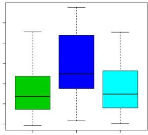
Comparative Box plots of Test Error

Figure 2: Comparison of the predictive performances. PCK seems to have a minute edge, but

clearly, the three methods are performing equally well on this data.

2.2

Second Artificial Example

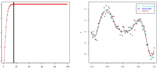
As our second artificial example, we consider exploring the hill function defined as

f(x) =₋x +√2 sin(π3/2x2) with x_∈[₋1,+1]

This function is somewhat qualitatively different from the previous one. Like before, we generate

0 20 40 60 80 100 0.2 0.4 0.6 0.8 1.0 number of components Propor tion of v ar iation captured −1.0 −0.5 0.0 0.5 1.0 −2 −1 0 1 2 x y + O − True Function Noisy data PCK fit

Figure 3: Results of the PCK algorithm for the hill function. The panel on the left shows

that our technique picks up around 16 relevant components. Note that this corresponding to essentially to the totality of the variation.

PCK SVM RVM 0.2 0.3 0.4 0.5 0.6 0.7

Comparative Box plots of Test Error

Figure 4: Comparison of the predictive performances. PCK seems to have a minute edge, but

clearly, the three methods are performing equally well on this data.

2.3

Real life example

The Boston housing data set is a well known benchmark data set often used to test the perfor-mance of regression methods.

PCK SVM RVM

Training Error 0.0002 0.0002 0.0001 Test Error 0.0174 0.0201 0.0181

For this data set, the Principal Component approach retains 49 relevant components. PCK SVM RVM 0.014 0.016 0.018 0.020 0.022 0.024

2.4

Summary of performances

Table 1: Comparison of the predictive performance of three methods based on the root mean

squared error on the test set. In this case, m = 50 replications is used each for each data set. The proposed method PCK is compared to both SVM and RVM

3

Conclusion

We have proposed a simple use of principal component analysis in feature space that allows the derivation of optimal predictive kernel regression. The proposed approach is shown to perform well on both artificial and real data. Despite its incredible simplicity, the proposed method is found to compete very well with sophisticated statistical approaches like the Relevance Vec-tor Machine and the Support VecVec-tor Machine. The proposed method merits to be considered seriously because of simplicity. An aspect worth investigating in our future work is the deriva-tion of way to trace back the relevant vectors themselves rather than settle with the relevant components.

References

[1] Tipping, M. E. (2001). Sparse Bayesian Learning and the Relevance Vector Machine.

Journal of Machine Learning Research,1, 211-244.

[2] Fokou´e, E. and Sun, D. and Goel, P.(2009). Fully Bayesian Analysis of the Relevance

Vector Machine with Consistency Inducing Priors. Statistical Methodology. Invited Paper,

to appear.

[3] Fokou´e, E.(2008). Estimation of Atom Prevalence for Optimal Prediction.Contemporary Mathematics. Vol443, pp 103-129, The American Mathematical Society.

[4] Fokou´e, E. (2008). Stabilization of Atom Selection for Optimal Prediction via Mixture

Modelling of the Sample Path.Technical Report. Number EPF-08-9-1_{. Department of}

Math-ematics, Kettering University, 1700 West Third Avenue, Flint, Michigan, USA. (2008)

Sub-mitted to Computational Statistics and Data Analysis

[5] Fokou´e, E. and P. Goel (2007). An Optimal Experimental Design Perspective on the

Relevance Vector Machine, Technical Report. Number EPF-07-12-1_{. Department of}

Mathe-matics, Kettering University, 1700 West Third Avenue, Flint, Michigan, USA.

[6] Zhang, Z., Jordan, M. I. and Yeung, D. (2008). Posterior Consistency of the

Sil-verman g-Prior in Bayesian Model Choice. Technical Report, Number xx_{, Department of}

Electrical Engineering and Computer Science, University of California, Berkeley, Califor-nia, USA.

[7] Scholkopf, B. and Smola, A.(2002). Learning with Kernels: Support Vector Machines, Regularization, Optimization and Beyond. MIT Press, 2002.

[8] Grandvalet, Y. (1998). Least absolute shrinkage is equivalent to quadratic penalization. In L. Niklasson,M. Boden, and T. Ziemske, editors, ICANN98, volume 1 of Perspectives in Neural Computing, pages 201206. Springer, 1998.

[9] Tibshirani, R. J. (1996). Regression Shrinkage and Selection via the LASSO.. J. Roy. Statist. Soc. Ser. B,58, 267-288.

[10] F. Liang and R. Paulo and G. Molina and M. Clyde and J. O. Berger(2008).

Mixtures of g-priors for Bayesian Variable Selection.J. Amer. Statist. Assoc.,103, 410-423.

[11] Wahba, G (2000). An Introduction to Model Building with Reproducing Kernel Hilbert

Spaces, Technical Report No. 1020, Department of Statistics, University of Wisconsin 1210