An Alternative System GMM Estimation in Dynamic Panel Models

Hi-Stat

Discussion Paper Series

No.217

An Alternative System GMM Estimation in Dynamic Panel Models

Hosung Jung Hyeog Ug Kwon

July 2007

Hitotsubashi University Research Unit for Statistical Analysis in Social Sciences A 21st-Century COE Program

Institute of Economic Research Hitotsubashi University Kunitachi, Tokyo, 186-8603 Japan http://hi-stat.ier.hit-u.ac.jp/

An Alternative System GMM Estimation in Dynamic

Panel Models

Hosung Jung

_{& Hyeog Ug Kwon}

July 22, 2007

Abstract

The system GMM estimator in dynamic panel data models which combines two moment conditions, i.e., for the differenced equation and for the model in levels, is known to be more efficient than the first-difference GMM estimator. However, an initial optimal weight matrix is not known for the system estimation procedure. Therefore, we suggest the use of ‘a suboptimal weight matrix’ which may reduce the finite sample bias whilst increasing its efficiency. Using the Kantorovich inequality, we find that the potential efficiency gain becomes large when the variance of indi-vidual effects increases compared to the variance of the idiosyncratic errors. (Our Monte Carlo experiments show that the small sample properties of the suboptimal system estimator are shown to be much more reliable than any other conventional system GMM estimator in terms of bias and efficiency.

Keywords: Dynamic panel data; sub-optimal weighting matrix; KI upper bound

1

Introduction

It is generally known that using many instruments can improve the efficiency of various IV and GMM estimators (Arellano and Bover, 1995; Blundell and Bond, 1998; Ahn and Schmidt, 1995; etc.). Therefore, the system GMM estimator in dynamic panel data models is more efficient than the first-difference GMM estimator.1 _{Despite the substantial}

efficiency gain, using many instruments has two important drawbacks: increased bias and unreliable inference (Newey and Smith, 2004; Hayakawa, 2005). In this paper, we investigate how to decrease bias while increasing efficiency in the system GMM estimation. Instead of adjusting the number of instrumental variables, we suggest an alternative way of improving efficiency.

In general, an asymptotically efficient estimator can be obtained through the two-step procedure in the standard GMM estimation. However, the estimated standard error can be biased downwards quite severely for moderate sample sizes, N (Windmeijer, 1998). It is obvious that the same problem persists even in the case of the two-step system GMM estimation. In practice, therefore, we often rely on an inference based on the less efficient one-step estimator, whose inference is much more reliable than that of the two-step estimator. Under this constraint, it becomes important to choose the weight matrix in the first step, especially in small samples. Unfortunately, the optimal weight matrix for the system estimator is only available when the variance of individual effects is

∗_{Samsung Economic Research Institute, e-mail:[email protected]} †_{Department of Economics, Nihon University, e-mail:[email protected]}

zero. Hence, we suggest using a suboptimal weight matrix which contains the estimated variance ratio of the individual effects to that of the idiosyncratic error term. This yields the suboptimal system GMM (SYSsub hereafter) estimation.2

To investigate the magnitude of the efficiency gain, KI upper bounds based on the Kantorovich inequality (Windmeijer, 1998) are applied. We find that the efficiency gain can potentially be large when the variance of individual effects increases. In addition, we conduct Monte Carlo studies to confirm the efficiency gain from using the SYSsub estimator when compared to the conventional system GMM estimation in Blundell and Bond (1998). While the small-sample properties of the conventional system estimators are heavily affected by the increase of the variance ratio, the SYSsubestimator is relatively reliable. As an empirical example, we estimate the Cobb-Douglas production function of a balanced panel of 1,002 Japanese manufacturing companies for the period 1991-2001.

The remainder of this paper is organized as follows. The next section presents the model and reviews the conventional system GMM estimation. In Section 2, we propose the SYSsubestimation and consider the efficiency gain against using the identity matrix as an initial weight matrix. Section 3 reports the simulation results, while Section 4 present an empirical application to a production function. Section 5 concludes. The notation is fairly standard and self-explanatory: ‘→’ denotes convergence in probability while ‘∼’ or ‘⇒’ is used for convergence in distribution. The nonstochastic limit of a sequence is also denoted by ‘→’ when the context makes the usage clear.

2

Models and the System GMM Estimator

To analyze the properties of the parameter estimators in the system GMM estimation, we consider a simple dynamic panel model with an autoregressive specification and a one-way error component, uit:

yit = αyit−1+uit, |α|<1. (1) uit = µi+vit (i= 1, . . . , N;t = 2, . . . , T), whereµi ∼iid ³ 0, σ2 µ ´

andvit ∼iid(0, σv2). To begin with, we assume thatµi andvithave the familiar error component structure in which

E(µi) = E(vit) =E(µivit) = 0 ∀ i, t (2)

and

E(vitvis) = 0. ∀ i, t6=s (3)

The yit series are assumed to be stationary and the series can alternatively be written as

yit = µi 1−α + ∞ X j=0 αj_v i,t−j (4)

We define the variance ratio,ρi = σ

2

µ

σ2

v, for later use. The system GMM estimator combines

moment conditions for the differenced equation with moment conditions for the model in levels. Adopting the standard assumptions concerning the error components (i.e., the white-noise error vit), Blundell and Bond (1998) noted the validity of the following ms = (T + 1)(T −2)/2 linear moment restrictions for each i,

E[yi,t−j∆uit] = 0 for (j = 2, . . . , t−1;t = 3, . . . , T) (5)

E[∆yi,t−1uit] = 0 for (t = 3, . . . , T). (6)

2_{As we need the first-step estimation to obtain the variance ratio, this estimation can be categorized} as a two-step GMM estimation. However, unlike the conventional two-step GMM estimation, we show that SYSsub does not suffer from a downward bias of its estimated standard error.

For convenience, the moment restrictions can be expressed more compactly as E[fi(α0)] =E(Zsi0 qi) = 0 (7) where qi = " ∆ui ui # . (8)

Zsi is a 2(T −2)×m block diagonal matrix given by

Zsi = " Zdi 0 0 Zli # (9) whereZdi and Zli refer to the instruments in the first-differenced equation and the levels equation, respectively. These are given by

Zdi=        [yi1] · · · 0 [yi1, yi2] ... . .. 0 · · · [yi1,· · ·, yiT−2]        (10) and Zli = diag[∆yi2,∆yi3, . . . ,∆yi,T−1]. (11)

Let Zs be a 2N(T −2)×ms matrix consisting of (Zs,1, . . . , Zs,N) and Y be a stacked matrixYi = (∆yi, yi). Then, the one-step system GMM estimator based on these moment conditions (7) is ˆ αs = h Y₋₁0 ZsWNZs0Y−1 i₋₁h Y₋₁0 ZsWNZs0Y i (12) for some positive weight matrix WN. The efficient two-step system GMM estimator is obtained in a similar way to the standard GMM procedure.

In panel data models, the estimated standard error can be substantially biased down-ward; therefore, we often rely on inference based on the less efficient one-step estimator. In this case, there is no one-step system GMM estimator that is asymptotically equivalent to the two-step estimator, unless σ2

µ = 0. As a natural choice for WN to yield the initial consistent estimator, Blundell and Bond (1998) used

WN = " 1 N N X i=1 Z0 siHsZsi #−1 , (13) where Hs = " Hd 0 0 IT−2 # . (14)

While the submatrix Hd–a (T −2) square matrix which has twos in the main diagonal, minus ones in the first subdiagonals, and zeros otherwise is used for the first-differenced equation, the identity matrix is used for the level estimation. This implies that the variance–covariance structure of residuals from the level estimation is not considered in the system estimation. Therefore, even if the weight matrix Hs works well for small values of σ2

3

A Suboptimal Weight Matrix

In large samples, the efficiency of the one-step system GMM estimator is not affected by the choice of the weight matrix, as long as the matrix is positive definite. Therefore, the efficiency gain for the two-step procedure may not be substantial asymptotically. However, there is no one-step system GMM estimator that is asymptotically equivalent to the two-step estimator, even in the special case of i.i.d. disturbances. Only in the case of σ2

µ= 0 is an optimal weight matrix for the system GMM estimator given by

Hs = " Hd C C IT−2 # (15) where C is a (T −2) square matrix which has ones in the main diagonal, minus ones in the first lower subdiagonals and zeros otherwise.3 _{Unless σ}2

µ = 0, the identity matrix IT−2 inHs should be replaced by the matrix JT−2 to achieve optimality, where

JT−2 =          1 +ρ ρ ρ · · · ρ ρ 1 +ρ ρ · · · ρ ρ ρ 1 +ρ · · · ρ ... ... ... . .. ... ρ ρ ρ · · · 1 +ρ          , (16)

which yields the optimal weight matrix, Hso:

Hso = " Hd C C JT−2 # . (17)

Although the system estimator in Blundell and Bond (1998) performs well as long as ρ

is reasonably small, there are always cases where the variance of the individual effects,

µi, is substantially larger than that of the classical error term,vit. The use of the weight matrixHso, therefore, can be described as inducing cross-sectional heterogeneity through ρ. Otherwise, using the matrix JT−2 can be explained as partially adopting a procedure

of GLS (generalized least squares) to the level estimation, which is not done in Blundell and Bond (1998). However, since the variance ratio,ρ, is unknown in practice, we suggest the estimate of the optimal weight matrix, Hso

c Hso = " Hd 0 0 JˆT−2 # , (18)

where a natural estimator for the variance ratio ˆρ is readily available in the initial step of the system estimation. To obtain ˆρ, we derive σ2

v from the first-difference GMM estimation, ˆ σ2 v = P_N i=1∆ˆu 0 i∆ˆui 2N(T −2) , (19) while σ2 µ is given by P_N i=1 h ˜ u0_iu˜i−∆˜u 0 i∆˜ui/2 i N(T −2) , (20)

where ∆ˆuiand ˜uiare residuals from the first difference and the level equation, respectively. Using this weight matrix, Hcso, instead of the matrix Hs, may improve the efficiency of the second-step system estimation when ρ becomes large.4

3_{Also see Windmeijer (1998) for details.}

4

Efficiency Gains

To measure the efficiency gain, we use the KI upper bounds. Using the moment condition (7), the system GMM estimator ˆαs for α0 minimizes

ˆ αs = argminα0 " 1 N N X i=1 fi(α) #0 WN " 1 N N X i=1 fi(α) # (21) whereWN is a positive definite weight matrix that satisfies N→∞WN =W. Furthermore, if we assume that

1

√

Nfi(α0)→N (0,Ψ), (22)

where the regularity conditions are in place and Fα = E(∂fi(α)/∂α), F0 ≡ Fα0, then √

N(ˆαs−α0) has a limiting normal distribution, √ N(ˆαs−α0)→N (0, VW), (23) where VW = (F 0 0W F0)−1F 0 0WΨW F0(F 0

0W F0)−1. An optimal choice for W is Ψ−1, so

the asymptotic variance matrix is given by (F₀0W F0)−1. Clearly, the following inequality

holds for any positive matrix W: (F₀0Ψ−1_F 0)−1 ≤(F 0 0W F0)−1F 0 0WΨW F0(F 0 0W F0)−1 (24)

According to Liu and Neudecker (1997), the following inequality also holds: (F₀0W F0)−1F 0 0WΨW F0(F 0 0W F0)−1 ≤ (λ1 +λp)2 4λ1λp (F₀0Ψ−1F0)−1, (25)

and the KI upper bounds – KIub = (λ1+λp)

2

4λ1λp – are calculated, where λi >0 (i = 1, . . . , p)

are the eigenvalues of the p×p matrix ΨW.5 _{If we use an initial weight matrix equal to}

ˆ Hso, Ψ is obtained by Ψ = 1 N N X i=1 h Z_i0HˆsoZi i , (26)

and the asymptotic variance matrix for using the suboptimal weighting matrix ˆHso then is (F₀0Ψ−1_F

0)−1. For T = 4, for example, with four overidentifying moment conditions,

the matrices Ψ and W1 are given by

Ψ = 1 N N X i=1 h Z_si0 HsoZsi i =          2σ2 y −σ2y −δ 0 0 −σ2 y 2σy2 2δ 0 0 −δ 2δ 2σ2 y 0 0 0 0 0 2(1+ρ)σ2v 1+α −ρ(1−α)σ2 v 1+α 0 0 0 −ρ(1−α)σv2 1+α 2(1+ρ)σ2 v 1+α          (27) and W1 = 1 N N X i=1 h Z_si0 Zsi i₋₁ =          σ2 y 0 0 0 0 0 σ2 y δ 0 0 0 δ σ2 y 0 0 0 0 0 2σ2v 1+α 0 0 0 0 0 2σ2v 1+α          −1 , (28)

where δ=σ2 y − σ 2 v 1+α. Hence, ΨW1 =          2 −1 0 0 0 −1 2 0 0 0 − δ σ2 y 0 2 0 0 0 0 0 (1 +ρ) −ρ(1−₂ α) 0 0 0 −ρ(1−₂ α) (1 +ρ)          . (29)

We easily find that the eigenvalues of the upper block matrix in (29) are 1,2 and 3, which are fixed for any values of δ andσ2

y. The eigenvalues of the lower block matrix are functions of ρ and α: λlow = " (1 +ρ)∓ −ρ(1−α) 2 # = ·_{2 + 3ρ−αρ} 2 , 2 +ρ+αρ 2 ¸ . (30)

If ρ ≤ 1.˙3, the eigenvalues of the lower block matrix in (29) are in [1,3] so that the

minimum and maximum of the eigenvalues of the whole matrix ΨW1 are 1 and 3,

respec-tively. This implies that the efficiency loss of the one-step system GMM estimator with the identity matrix is around 30% compared to the suboptimal system GMM estimator.

5

Monte Carlo Experiments

This section illustrates the small-sample performance of the various system GMM esti-mators. Monte Carlo experiments were carried out based on a data generating process following Nerlove (1971) and Blundell and Bond (1998).

yit =αyit−1+uit, (31)

for i = 1,2, . . . , N and t = 2,3, . . . , T. For the random-effects specification, we generate

uit = µi +vit, where µi ∼ iid(0, σ2µ). All the innovations are independent over time and are homoscedastic; that is, vit∼NID(0,1). We generate the initial conditions yi1 as

yi1 =

µi

1−α +wi1, (32)

where wi1 is an NID(0, σw1) random variable, independent of both µi and vit with the variance σw1 chosen to satisfy covariance stationarity.

The variance ratio,ρ, is characterized by σµ2

σ2

v, so it depends only onσ 2

µ. Throughout the experiments, eighteen parameter settings (i.e., α = 0.2,0.5,0.8 and ρ= 0,0.5,1,2,5,10) are simulated. To compare the small-sample performance, the five different system GMM estimation procedures are considered according to their weight matrix. Specifically, ISYS denotes the first-step estimator, which uses the identity matrix, while the one- and two-step system GMM estimation in Blundell and Bond (1998) are named SYS1 and SYS2,

respectively. Furthermore, SYS3 uses the alternative suboptimal weighting matrix defined

in (15). SYSsub denotes the newly proposed suboptimal weight matrix (18), which uses the estimated ρ, while TSYSsub uses the trueρ.6

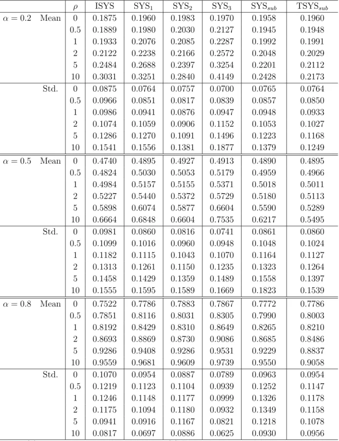
Tables 1 and 2 present the estimation results for T = 5 and 10, respectively. Clearly, the bias and the standard deviations of all the estimators are affected by the variance ratio ρ. While the biases of ISYS, SYS1, SYS2 and SYS3 are negligible whenρ≤1, they

6_{In one of the most widespread statistics programs, STATA, ISYS, SYS}

1 and SYS3 are derived by choosingh(1), h(2) andh(3), which determine the first-step weight matrix from among three options.

Table 1: Small-sample properties of various GMM estimators (T=5)

ρ ISYS SYS1 SYS2 SYS3 SYSsub TSYSsub

α= 0.2 Mean 0 0.1875 0.1960 0.1983 0.1970 0.1958 0.1960 0.5 0.1889 0.1980 0.2030 0.2127 0.1945 0.1948 1 0.1933 0.2076 0.2085 0.2287 0.1992 0.1991 2 0.2122 0.2238 0.2166 0.2572 0.2048 0.2029 5 0.2484 0.2688 0.2397 0.3254 0.2201 0.2112 10 0.3031 0.3251 0.2840 0.4149 0.2428 0.2173 Std. 0 0.0875 0.0764 0.0757 0.0700 0.0765 0.0764 0.5 0.0966 0.0851 0.0817 0.0839 0.0857 0.0850 1 0.0986 0.0941 0.0876 0.0947 0.0948 0.0933 2 0.1074 0.1059 0.0906 0.1152 0.1053 0.1027 5 0.1286 0.1270 0.1091 0.1496 0.1223 0.1168 10 0.1541 0.1556 0.1381 0.1877 0.1379 0.1249 α= 0.5 Mean 0 0.4740 0.4895 0.4927 0.4913 0.4890 0.4895 0.5 0.4824 0.5030 0.5053 0.5179 0.4959 0.4966 1 0.4984 0.5157 0.5155 0.5371 0.5018 0.5011 2 0.5227 0.5440 0.5372 0.5729 0.5180 0.5113 5 0.5898 0.6074 0.5877 0.6604 0.5590 0.5289 10 0.6664 0.6848 0.6604 0.7535 0.6217 0.5495 Std. 0 0.0981 0.0860 0.0816 0.0741 0.0861 0.0860 0.5 0.1099 0.1016 0.0960 0.0948 0.1048 0.1024 1 0.1182 0.1115 0.1043 0.1070 0.1164 0.1127 2 0.1313 0.1261 0.1150 0.1235 0.1323 0.1264 5 0.1458 0.1429 0.1359 0.1489 0.1558 0.1397 10 0.1555 0.1595 0.1589 0.1669 0.1823 0.1539 α= 0.8 Mean 0 0.7522 0.7786 0.7883 0.7867 0.7772 0.7786 0.5 0.7851 0.8116 0.8031 0.8305 0.7990 0.8003 1 0.8192 0.8429 0.8310 0.8649 0.8265 0.8210 2 0.8693 0.8869 0.8730 0.9086 0.8685 0.8486 5 0.9286 0.9408 0.9286 0.9531 0.9229 0.8837 10 0.9559 0.9681 0.9609 0.9739 0.9550 0.9058 Std. 0 0.1070 0.0954 0.0887 0.0789 0.0963 0.0954 0.5 0.1219 0.1123 0.1104 0.0939 0.1252 0.1147 1 0.1246 0.1148 0.1177 0.0999 0.1326 0.1178 2 0.1175 0.1094 0.1180 0.0932 0.1349 0.1158 5 0.0941 0.0916 0.1167 0.0821 0.1218 0.1078 10 0.0817 0.0697 0.0886 0.0625 0.0930 0.0956

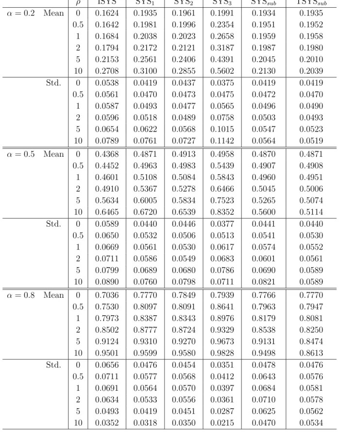
Table 2: Small-sample properties of various GMM estimators (T=10)

ρ ISYS SYS1 SYS2 SYS3 SYSsub TSYSsub

α= 0.2 Mean 0 0.1624 0.1935 0.1961 0.1991 0.1934 0.1935 0.5 0.1642 0.1981 0.1996 0.2354 0.1951 0.1952 1 0.1684 0.2038 0.2023 0.2658 0.1959 0.1958 2 0.1794 0.2172 0.2121 0.3187 0.1987 0.1980 5 0.2153 0.2561 0.2406 0.4391 0.2045 0.2010 10 0.2708 0.3100 0.2855 0.5602 0.2130 0.2039 Std. 0 0.0538 0.0419 0.0437 0.0375 0.0419 0.0419 0.5 0.0561 0.0470 0.0473 0.0475 0.0472 0.0470 1 0.0587 0.0493 0.0477 0.0565 0.0496 0.0490 2 0.0596 0.0518 0.0489 0.0758 0.0503 0.0493 5 0.0654 0.0622 0.0568 0.1015 0.0547 0.0523 10 0.0789 0.0761 0.0727 0.1142 0.0564 0.0519 α= 0.5 Mean 0 0.4368 0.4871 0.4913 0.4958 0.4870 0.4871 0.5 0.4452 0.4963 0.4983 0.5439 0.4907 0.4908 1 0.4601 0.5108 0.5084 0.5843 0.4960 0.4951 2 0.4910 0.5367 0.5278 0.6466 0.5045 0.5006 5 0.5634 0.6005 0.5834 0.7523 0.5265 0.5074 10 0.6465 0.6720 0.6539 0.8352 0.5600 0.5114 Std. 0 0.0589 0.0440 0.0446 0.0377 0.0441 0.0440 0.5 0.0650 0.0532 0.0506 0.0513 0.0541 0.0530 1 0.0669 0.0561 0.0530 0.0617 0.0574 0.0552 2 0.0711 0.0586 0.0549 0.0683 0.0601 0.0561 5 0.0799 0.0689 0.0680 0.0786 0.0690 0.0589 10 0.0890 0.0760 0.0798 0.0711 0.0821 0.0589 α= 0.8 Mean 0 0.7036 0.7770 0.7849 0.7939 0.7766 0.7770 0.5 0.7530 0.8097 0.8091 0.8641 0.7963 0.7947 1 0.7973 0.8387 0.8343 0.8976 0.8179 0.8081 2 0.8502 0.8777 0.8724 0.9329 0.8538 0.8250 5 0.9124 0.9310 0.9270 0.9673 0.9131 0.8474 10 0.9501 0.9599 0.9580 0.9828 0.9498 0.8613 Std. 0 0.0656 0.0476 0.0454 0.0351 0.0478 0.0476 0.5 0.0711 0.0577 0.0568 0.0412 0.0643 0.0576 1 0.0691 0.0564 0.0570 0.0397 0.0684 0.0581 2 0.0634 0.0533 0.0556 0.0361 0.0710 0.0578 5 0.0493 0.0419 0.0451 0.0287 0.0625 0.0562 10 0.0352 0.0318 0.0350 0.0215 0.0470 0.0534

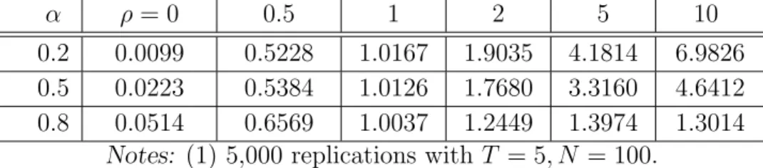
Table 3: Estimation Results of ρ

α ρ= 0 0.5 1 2 5 10

0.2 0.0099 0.5228 1.0167 1.9035 4.1814 6.9826

0.5 0.0223 0.5384 1.0126 1.7680 3.3160 4.6412

0.8 0.0514 0.6569 1.0037 1.2449 1.3974 1.3014

Notes: (1) 5,000 replications with T = 5, N = 100.

rapidly increase with ρ. The biases of SYSsub and TSYSsub show a much slower increase due to an increase inρ. Even in the case ofα = 0.8, the two estimators show the smallest increase in mean. On the other hand, SYSsub and TSYSsub in most cases have smaller variance than any of the other estimators except SYS2.7 Consequently, we conclude that

SYSsub outperforms the conventional system estimators in terms of bias and efficiency. However, the advantage of the SYSsub estimator decreases as α grows to unity because a high α leads to an unreliable estimate of ρ itself.

Table 3 presents the estimation results of ρ based on residuals from the first-step system GMM estimator. The mean of the estimated ρ has substantial bias when α is close to one, which yields no considerable improvement to using the suboptimal system procedure. Even though the suggested estimator, SYSsub, depends on the results from the first-step estimation ofρ, in most cases, SYSsubperforms better than any of the other conventional system estimators widely in use.

6

Empirical Application: Estimation of Production

Functions using Japanese Firm-level Panel Data

We apply the suboptimal system GMM estimation procedure (denoted SYSsub) to the es-timation of production functions using firm-level balanced panel data for 1,002 Japanese manufacturing firms. As highlighted by Griliches and Mairesse (1995), there are many econometric problems involved in the estimation of production functions, including un-observed heterogeneity between firms, simultaneity of the decisions about inputs and output, and measurement errors in inputs. We compare our result with the results from the different estimation approaches that have been proposed to deal with these problems, such as OLS, LSDV, GMM and system GMM.

We estimate

yit = βmMit+βlLit+βkKit+γt+ (µi+vit+mit) (33)

vit = αvi,t−1+eit |α|<1, (34)

where yit is the log of firm i’s sales in year t,Mit is the log of intermediate inputs, Lit is the log of employment, Kit is the log of capital stock, and γt is a year-specific intercept reflecting, for example, a common technology shock. As for the error components, µi is an unobserved firm-specific effect, vit is a possibly autoregressive productivity shock, and mit is measurement error. We assume that mit and eit are serially uncorrelated. As all independent variables are potentially correlated with the individual-specific effects and with productivity shocks, no valid moment conditions for specification (34) exist as long as α6= 0. However, this model has a dynamic common factor representation:

yit=αyi,t−1+βmMit−αβmMi,t−1+βlLit−αβlLi,t−1+βkKit−αβkKi,t−1 (35)

+(γt−αγt−1) + (µi(1−α) +eit+mit−αmi,t−1)

or

yit =π1yi,t−1+π2Mit+π3Mi,t−1+π4Lit+π5Li,t−1+π6Kit+π7Ki,t−1 (36)

˙

γt+ ( ˙µi+wit),

subject to the three nonlinear common factor restrictions π3 = −π1π2, π5 = −π1π4

and π7 =−π1π6. On the other hand, the error term wit =eit+mit−αmi,t−1 is serially

uncorrelated if there are no measurement errors orwit∼MA(1) if there are measurement errors in some of the series. Although consistent estimates of the unrestricted parameters,

π = (π1, . . . , π7), are possible in either case, we assume there is no measurement error,

i.e., mit = 0, for convenience. Using the suboptimal system GMM methods outlined in the previous sections, we present the consistent estimates of π and var(π).

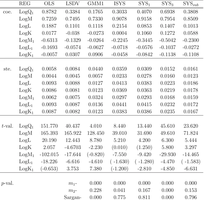
Table 4 presents the various estimation results. The key element we are interested in is the sign of the coefficient estimates and their significance. Typically, the coefficients of labor, capital, and intermediate inputs will tend to be biased upward in pooled OLS, whereas the LSDV estimator controlled for unobserved heterogeneity provides very small estimates of capital (see the survey by Griliches and Mairesse (1995)).

In the estimation results reported in Table 4, the value of the LSDV estimate of capital is negative but significant. The low coefficient on capital may be caused by measure-ment errors in the calculation of capital stocks and the difficulty of rapid adjustmeasure-ments in response to exogenous shocks like demand shifts or productivity shocks. Our result obtained by the LSDV estimator is consistent with previous findings by Blundell and Bond (1998) and Black and Lynch (2001).

In order to control for these two problems, the first differences GMM (denoted GMM1)is used in the estimation of the production function. Unfortunately, the first differences GMM does not remedy the two distortions of the LSDV estimator, showing that the esti-mated coefficient of capital is smaller than that of the LSDV estimation. Overidentifying restrictions are also rejected. These findings result from the weak instruments problem in dynamic models where regressors in first differences are weakly autocorrelated and from the exacerbation of the measurement error problem caused by the elimination of the cross-sectional variation through first differencing.

These findings indicate that the measurement error downward bias in capital is clearly in excess of the upward bias caused by simultaneity. Blundell and Bond (2000) suggest an alternative estimator that corrects these problems in the first differenced GMM estima-tors, which they called the system GMM. Blundell and Bond (2000) and Alonso-Borrego and Sanchez-Mangas (2001), using UK and Spanish data, respectively, show that the system GMM estimation performs very well. In the system GMM estimation, the equa-tion in differences is instrumented by lagged differences (while the equaequa-tion in levels is additionally instrumented by suitably lagged differences. A reason that the system GMM works better than the first differenced GMM is that the second set of moment conditions reduces weak instruments problems and the large measurement error in capital.

Table 4 also reports the coefficient estimates from three different methods of the sys-tem GMM. When applying the syssys-tem GMM using the one-step identity weight matrix (ISYS), we obtained the result that the coefficients on the lagged dependent variable and capital were larger than those of the first differenced GMM. The Sargan-statistic does not reject the validity of the instruments. However, the coefficient on capital is not still significant. Even when using SYS1, we still found a large coefficient on the lagged

depen-dent variable and an insignificant coefficient on capital, while the coefficient on labor was considerably smaller than the result of ISYS, which is an unexpected result. By contrast, the specification of SYS3 corrects for large measurement error in the differences of capital

Table 4: Results of the Estimation of the Cobb-Douglas Production Function

REG OLS LSDV GMM1 ISYS SYS1 SYS3 SYSsub

coe. LogQ1 0.8782 0.3384 0.1765 0.3033 0.4070 0.6938 0.3808 LogM 0.7259 0.7495 0.7330 0.9078 0.9158 0.7954 0.8509 LogL 0.1887 0.1101 0.1118 0.2154 0.0853 0.1407 0.1013 LogK 0.0177 -0.038 -0.0273 0.0004 0.1060 0.1272 0.0588 LogM1 -0.6313 -0.1329 -0.0264 -0.2245 -0.3445 -0.5042 -0.2300 LogL1 -0.1693 -0.0574 -0.0627 -0.0718 -0.0576 -0.1037 -0.0272 LogK1 -0.0057 0.0307 0.0906 -0.0458 -0.0842 -0.1138 -0.1108 ste. LogQ1 0.0058 0.0084 0.0440 0.0359 0.0309 0.0152 0.0161 LogM 0.0044 0.0045 0.0057 0.0233 0.0278 0.0160 0.0123 LogL 0.0093 0.0088 0.0127 0.0413 0.0383 0.0223 0.0186 LogK 0.0086 0.0081 0.0123 0.0369 0.0363 0.0219 0.0178 LogM1 0.0062 0.0075 0.0324 0.0297 0.0293 0.0168 0.0159 LogL1 0.0093 0.0087 0.0136 0.0441 0.0415 0.0232 0.0172 LogK1 0.0087 0.0082 0.0123 0.0383 0.0386 0.0235 0.0167 t-val. LogQ1 151.770 40.437 4.010 8.440 13.440 45.610 23.620 LogM 165.393 165.922 128.450 39.010 31.690 49.610 71.824 LogL 20.190 12.443 8.780 5.210 4.200 6.300 5.444 LogK 2.057 -4.6703 -2.230 (0.010) (1.250) 5.800 3.297 LogM1 -102.015 -17.644 (-0.820) -7.550 -9.420 -29.930 -14.465 LogL1 -18.226 -6.616 -4.610 ( -1.630) ( -1.280) -4.470 ( -1.583) LogK1 (-0.653) 3.753 7.380 (-1.200) -2.810 -4.850 -6.631 p-val. m1- 0.000 0.000 0.000 0.000 0.000 m2- 0.228 0.041 0.167 0.000 0.153 Sargan- 0.000 0.775 0.811 0.000 0.796

Notes: (1) The year dummy included in the estimation is not reported here. (2) 5% critical values are used in the specification tests. (3) ISYS, SYS1 and SYS3 are based

on their one-step estimation. (4) The initially estimated value, ˆρ = 3.6237, is used for SYSsub. (5) LogQ1 refers to the lagged levels at t−1.

accepted. This indicates that the system GMM estimator using SYS3 will be inconsistent

The limitation of the system GMM is that it cannot obtain consistent estimates because it does not consider the fixed effects in level equation.

The results show that the alternative estimation suggested in this paper helps to alleviate the econometric problems in the estimation of production functions such as unobserved heterogeneity, simultaneity, and measurement errors in intermediate inputs. For example, the estimate of the coefficient on capital is positive and significant, while the coefficient on inputs is quite realistic. The specification tests suggest that no second order correlation in the error terms is present and that the instruments are valid. In sum, our estimation results clearly show that the suboptimal system GMM estimator performs very well when compared with the first differences GMM or the three other system GMM estimators.

7

Conclusion

The weak instruments problem may cause substantial small-sample biases when using the first-difference GMM procedure to estimate autoregressive models for moderately persistent series from short panels. (Also see Blundell and Bond,1998). However, these biases could be reduced by incorporating more informative moment conditions that are valid under quite general stationarity restrictions on the initial conditions. To this end, the system GMM estimation using lagged first differences as instruments for equations in addition to the usual lagged levels as instruments for the first differences equations is suggested as an alternative in Blundell and Bond (1999).

To go one step further, we considered a suboptimal system GMM estimation in the analysis of dynamic panel data sets with large cross-sectional variance. Since the small-sample properties of the first-difference GMM estimators depend on the initial weighting matrix, the performance of various system estimators with different weight matrices was investigated. Our Monte Carlo results indicate that the conventional system estimators are vulnerable to an increase inρ.One of the most distinguishing features in these experi-ments was that biases and standard deviations increase withρin most cases. To overcome this deficiency, by inducing the variance of individual effects, µi, into the weight matrix, the SYSsub estimation successfully weakens the increase of its biases and variances. Con-sequently, we expect that the SYSsub estimation will provide useful parameter estimates for the practitioner.

In the estimation of the Cobb-Douglas production function for the 1,002 Japanese manufacturing firms, the suggested estimator provides the best parameter estimates in terms of precision.

Acknowledgement

The first author would like to thank Professor Katsuto Tanaka, Professor Taku Yamamoto and Doctor Kyongwon Kim for suggestions and valuable comments. We gratefully ac-knowledge the Grant-in-Aid from New Energy and Industrial Technology Development Organization (grant no. 0624006)

Appendix

The source of our data on Japanese manufacturing firms for the empirical application is the DBJ database compiled by the Development Bank of Japan

Output: Firms’ total sales are used as a proxy for gross output. Total sales are deflated by output deflators obtained from the SNA (System of National Accounts).

Intermediate inputs: Intermediate inputs are defined as (Cost of sales + Operating costs) - (Wages + Depreciation costs) and are provided in the SNA.

Labor input: As labor input, we used the average of man hours between year t and year t-1. Man hours are computed as each firms’ total number of workers multiplied by the sectoral working hours obtained from the JIP.

The JIP 2006 Database was compiled as part of a RIETI research project. The detailed results of this project are reported in Fukao et al. (2006). The database contains annual information on 108 sectors, including 56 non-manufacturing sectors, from 1970 to 2002. These sectors cover the whole Japanese economy. The database includes detailed information on factor inputs, annual nominal and real input-output tables, as well as some additional statistics, such as capacity utilization rates, Japan’s international trade by trade partner, inward and outward FDI, etc., at the detailed sectoral level. An Excel file version of the JIP2006 Database is available on RIETI’s web site.

References

[1] Ahn, S.C and P. Schmidt, 1995, Efficient estimation of models for dynamic panel data, Journal of Econometrics 68, 29-52.

[2] Amemiya, T., 1976, The maximum likelihood, the minimum chi-square and the non-linear weighted least squares estimator in the general qualitative response model,

Journal of the American Statistical Association 71, 347-351.

[3] Alonso-Borrego, C. and R. Sanchez-Mangas, 2001, GMM Estimation of a Production Function with Panel Data: An Application to Spanish Manufacturing Firms,Statistics

and Econometrics Working Papers ws015527, Universidad Carlos III.

[4] Anderson, T.W. and C. Hsiao, 1981, Estimation of dynamic models with error com-ponents, Journal of the American Statistical Association 76, 598-606.

[5] Anderson, T.W. and C. Hsiao, 1982, Formulation and estimation of dynamic models using panel data, Journal of Econometrics 18, 47-82.

[6] Arellano, M. and S. Bond, 1991, Some tests of specification for panel data: Monte Carlo evidence and an application to employment equations, Review of Economic Studies 58, 277-297.

[7] Arellano, M. and O. Bover, 1995, Another look at the instrumental variable estimation of error-components models, Journal of Econometrics 68, 29-52.

[8] Balestra, P. and M. Nerlove, 1966, Pooling cross-section and time series data in the estimation of a dynamic model: the demand for natural gas, Econometrica 34, 585-612.

[9] Baltagi, B.H. and Q. Li, 1995, Testing AR(1) against MA(1) disturbances in an error component model, Journal of Econometrics 48, 385-393.

[10] Bhargava, A., L. Franzini and W. Narendranathan, 1982, Serial Correlation and Fixed effects model, Review of Economic Studies 49, 533-549.

[11] Bhargava, A. and J.D. Sargan, 1983, Estimating dynamic random-effects models from panel data covering short time periods, Econometrica51, 1635-1659.

[12] Black, S. E. and L. M. Lynch, 2001, How to Compete: The Impact of Work-place Practices and Information Technology on Productivity,Review of Economics and Statistics 83, 435-445.

[13] Blundell, R. and R.J. Smith, 1991, Conditions Initiales et Estimation Efficace dans les Modeles Dynamiques sur Donnees de Panel: une Application au Comportement d’Invetissement des Enterprises,Annales d’Economie et de Statistique20/21, 109-123. [14] Blundell, R. and S. Bond, 1998, Initial conditions and moment restrictions in

dy-namic panel data models, Journal of Econometrics 87, 115-143.

[15] Bowsher, G. 2002, On testing overidentifying restrictions in dynamic panel data models, Economics Letters 77, 211-220.

[16] Fukao, K., S. Hamagata, T. Inui, K. Ito, H.U. Kwon, T. Makino, T. Miyagawa, Y. Nakanishi, and J. Tokui, 2006, Estimation Procedures and TFP Analysis of the JIP Database 2006 Provisional Version, paper presented at the EU KLEMS 3rd Consor-tium Meeting, May 7-9, 2006, Valencia (Spain).

[17] Harris, M.N. and Laszlo Matyas, 2001, The Robustness of Estimators for Dynamic Panel Data Models to Misspecification, (Monash University, Dept. of Econometrics), Working Paper no. 9/96.

[18] Griliches Z. and Mairesse, 1995, Production Functions: The Search for Identification, NBER Working Paper No.8075.

[19] Hausman, J.A. and W. E. Taylor, 1981, Panel Data and Unobservable Individual Effects, Econometrica49, 1377-1398.

[20] Hayakawa, K, 2005, Small Sample Bias Properties of the System GMM Estimators in Dynamic Panel Data Models, Hi-Stat Discussion Paper Series No.82, Hitotsubashi University, Tokyo.

[21] Hsiao, C., 1986, Analysis of Panel Data ( Cambridge University Press, Cambridge). [22] Keane, M.P. and D.E. Runkle, 1992, On the estimation of panel data models with serial correlation when instruments are not strictly exogenous, Journal of Business and Economic Statistics 10, 1-9.

[23] Kiviet, J.F, 1995, On bias, inconsistency and efficiency in various estimators of dynamic panel data models, Journal of Econometrics 68, 53-78.

[24] Liu, S. and H. Neudecker, 1997, Experiments with Mixtures: Optimal Allocations for Becker’s Models, Metrika 45, 53-66.

[25] Nerlove, M., 1971a, Further evidence on the estimation of dynamic economic rela-tions from a time series of cross-secrela-tions, Econometrica39, 359-382.

[26] Newey, W. K. and R.J. Smith, 2004, Higher Order Properties of GMM and Gener-alized Empirical Likelihood Estimators, Econometrica 72, 219-255.

[27] Nickell, S., 1981, Biases in dynamic models with fixed effects , Econometrica 49, 1399-1416.

[28] Wansbeek, T.J. and P. Bekker, 1996, On IV, GMM and ML in a dynamic panel data model, Economics Letters 51, 145-152.

[29] Windmeijer, F., 2004, A finite sample correction for the variance of linear efficient two-step GMM Estimator, Journal of Econometrics, Forthcoming.