Quantile Forecasting of Commodity Futures' Returns: Are Implied Volatility Factors Informative?

(1)

QUANTILE FORECASTING OF COMMODITY FUTURES’ RETURNS: ARE IMPLIED VOLATILITY FACTORS INFORMATIVE?

A Thesis by

MIGUEL EDUARDO DORTA

Submitted to the Office of Graduate Studies of Texas A&M University

in partial fulfillment of the requirements for the degree of MASTER OF SCIENCE

May 2012

(2)

Quantile Forecasting of Commodity Futures’ Returns: Are Implied Volatility Factors Informative?

(3)

QUANTILE FORECASTING OF COMMODITY FUTURES’ RETURNS: ARE IMPLIED VOLATILITY FACTORS INFORMATIVE?

A Thesis by

MIGUEL EDUARDO DORTA

Submitted to the Office of Graduate Studies of Texas A&M University

in partial fulfillment of the requirements for the degree of

MASTER OF SCIENCE

Approved by:

Co-Chairs of Committee, Ximing Wu Joshua Woodard Committee Member, Jamis Perrett Head of Department, John P. Nichols

May 2012

(4)

ABSTRACT

Quantile Forecasting of Commodity Futures’ Returns: Are Implied Volatility Factors Informative? (May 2012) Miguel Eduardo Dorta, B.S., Universidad Central de Venezuela;

M.S., University of Illinois at Urbana-Champaign Co-Chairs of Advisory Committee: Dr. Ximing Wu Dr. Joshua Woodard

This study develops a multi-period log-return quantile forecasting procedure to evaluate the performance of eleven nearby commodity futures contracts (NCFC) using a sample of 897 daily price observations and at-the-money (ATM) put and call implied volatilities of the corresponding prices for the period from 1/16/2008 to 7/29/2011. The statistical approach employs dynamic log-returns quantile regression models to forecast price densities using implied volatilities (IVs) and factors estimated through principal component analysis (PCA) from the IVs, pooled IVs and lagged returns. Extensive in-sample and out-of-in-sample analyses are conducted, including assessment of excess trading returns, and evaluations of several combinations of quantiles, model

specifications, and NCFC’s. The results suggest that the IV-PCA-factors, particularly pooled return-IV-PCA-factors, improve quantile forecasting power relative to models using only individual IV information. The ratio of the put-IV to the call-IV is also found to improve quantile forecasting performance of log returns. Improvements in quantile

(5)

forecasting performance are found to be better in the tails of the distribution than in the center. Trading performance based on quantile forecasts from the models above

generated significant excess returns. Finally, the fact that the single IV forecasts were outperformed by their quantile regression (QR) counterparts suggests that the

(6)

TABLE OF CONTENTS

Page

ABSTRACT ... iii

TABLE OF CONTENTS ... v

LIST OF FIGURES ... vi

LIST OF TABLES ...vii

1. INTRODUCTION ... 1 1.1 Motivation ... 1 1.2 Literature Review ... 3 1.3 Objectives ... 8 2. METHODOLOGY ... 10 2.1 General Strategy ... 10 2.2 Methods ... 12 3. EMPIRICAL ANALYSIS ... 21

3.1 Description of the Data ... 21

3.2 Quantile Regressions Model Specifications ... 21

3.3 Quantile Regressions Estimations and In-Sample Analysis ... 26

3.4 Out-of-Sample Quantile Forecasting Performance ... 34

4. CONCLUSION ... 43

REFERENCES ... 45

APPENDIX ... 49

(7)

LIST OF FIGURES

Page

Figure 1. Corn: put-IV (CCCP) and call-IV (CCCC) ... 22

Figure 2. Corn: log-return (rCCCS) and IV-ratio (RCCC) ... 23

Figure 3. Light crude oil: put-IV (CLNCP) and call-IV (CLNCC) ... 23

(8)

LIST OF TABLES

Page Table 1. Summary Statistics (selected commodities) ... 22 Table 2. Quantile Regressions of Log-Returns by Type of Period. Relative

Frequencies of Statistical Significance (5% level) of Explanatory Variables. Combined Commodities and Quantiles. ... 27 Table 3. Quantile Regressions of Daily Returns by Density Region. Relative

Frequencies of Statistical Significance (5% level) of Explanatory Variables. Combined Commodities and Quantiles. ... 29 Table 4. Quantile Regressions of Weekly Returns by Density Region. Relative

Frequencies of Statistical Significance (5% level) of Explanatory Variables. Combined Commodities and Quantiles. ... 30 Table 5. Quantile Regressions of Monthly Returns by Density Region. Relative

Frequencies of Statistical Significance (5% level) of Explanatory Variables. Combined Commodities and Quantiles. ... 31 Table 6. Quantile Regressions of Daily Returns. Relative Frequencies of Statistical

Significance (5% level) of Explanatory Variables. Top Commodities and Models Specifications. ... 32 Table 7. Quantile Regressions of Weekly Returns. Relative Frequencies of Statistical

Significance (5% level) of Explanatory Variables. Top Commodities and Models Specifications. ... 32 Table 8. Quantile Regressions of Montly Returns. Relative Frequencies of Statistical

Significance (5% level) of Explanatory Variables. Top Commodities and Models Specifications. ... 33 Table 9. Out-of-Sample Performance of Quantile Regressions, Black-Scholes, and

GARCH models. Hit% Deviations and Dynamic Quantile Test Relative Frequency of Rejection. By Model Specification and Type of Own-Implied Volatility. ... 35 Table 10. Out-of-Sample Performance of Quantile Regressions, Black-Scholes, and

GARCH. Hit% Deviations and Dynamic Quantile Test Relative Frequency of Rejection. By Distribution Region, Model Specification, and Type of Own-Implied Volatility. ... 37

(9)

Page Table 11. Out-of-Sample Performance of Quantile Regressions, Black-Scholes, and

GARCH models. Hit% Deviations and Dynamic Quantile Test Relative Frequency of Rejection. By Commodity Future Contract and Model

Specification. ... 39 Table 12. Out-of-Sample Excess Returns Generated by Long Trading Rules Based on

Some of the Quantiles Forecasted by Quantile Models. Equally Weighted Portfolio of Commodities. Average Daily Percentages. ... 41 Table A1. Eigenvalues of the Correlation Design Matrices (selected commodities) ... 50

(10)

1. INTRODUCTION

1.1 Motivation

This study develops a multi-period log-return quantile forecasting procedure to evaluate the performance of eleven nearby commodity futures contracts (NCFC) using a sample of 897 daily price observations and at-the-money (ATM) put and call implied volatilities of the corresponding prices for the period from 1/16/2008 to 7/29/2011. The motivation for focus on quantiles and quantile regressions is based on the observation that the typical Gaussian distribution assumption for log-returns is likely to be inadequate to describe the distributions of real prices changes. If the true distribution of asset log-returns has excess kurtosis or skewness, Gaussian based forecast could overexpose investors to financial risk. GARCH-class models, extensively used for log-returns density forecasting, have a somewhat limited ability to allow higher moments to be time-varying; and, they are not well suited for incorporating forward-looking expectations as they are all derived from information on historical prices. In contrast, forward-looking expectations of volatility are likely to be better captured from the futures and options markets, particularly through implied volatilities (IVs). In the context of non-parametric density forecasting, one approach for directly forecasting quantiles without assuming a particular theoretical model for the density is quantile regression (QR). However, nearly all existing studies have applied this idea in single commodity frameworks. Also, to our ____________

(11)

knowledge, this method has not been sufficiently investigated for adoption in commodity futures markets.

Principal component analysis (PCA) and similar factor extraction methods are used as independent variables in the QR model, as changes in volatilities among multiple markets may contain information that can improve density forecasting in related

markets. To our knowledge no studies have attempted to combine information from multiple markets extracted from PCA factors for use in QR density forecasts. The Black-Scholes (BS) (1973) option pricing model, which is based on the assumption of a log-normal density and risk-neutrality, would coincide with the true only if the underlying price process is a Brownian motion. Hence, differences between BS-derived put-IVs versus BS-derived call-IVs, may contain information about skewness and kurtosis of the log-returns.

Undertaking these issues, this study develops a QR model to forecast log-return quantiles of NCFC’s. The proposed statistical strategy for the return density forecasting is based on specifying and fitting QR models of log-returns using IVs and factors estimated through PCA from IVs. Augmenting the QR model by conditioning on information contained in IVs can be viewed as a way of accommodating forward-looking expectations of volatility, and is likely to outperform the use of historical prices alone. This approach to density forecasting of NCFC’s log-returns may serve as a

complementary tool for risk management purposes in the trading industry, to agricultural businesses, as well as in finance.

(12)

1.2 Literature Review

Numerous studies in finance have investigated density characteristics of asset returns, in light of the consistent empirical evidence that the normal distribution seems to be inadequate to describe their mechanics. Many empirical investigations have used non-normal distributions in order to model the density of stocks, foreign exchange, and commodity futures (CF) log-returns (Bollerslev 1987; Jorion 1988; Baillie and Bollerslev 1989; Nelson 1991; Giot and Laurent 2003; Kuester et al. 2006; Fuss et al. 2010), giving special consideration to the excess kurtosis and skewness.

The demand for accurate distributional forecasts in risk management has grown rapidly in recent years. Corporations such as J. P. Morgan, Reuters, and Bloomberg regularly engage in the estimation of density forecasts in order to value tailored

portfolios and derivatives. In this context, the focus of attention is typically on the tail of the density. In this sense, if distributional assumptions are incorrect, VaR forecasts will be misleading. For instance, if the true distribution of an asset's log-returns has excess kurtosis, then VaR’s computed under the assumption of normality will be overestimated. Hedgers and regulators are also concerned about forecasting the density of asset returns. For example, the Bank for International Settlements requires a bank to hold capital to cover losses on its trading portfolios in times of financial distress. Furthermore, the interest in density forecasting is also great in other financial applications such as portfolio optimization and option pricing. For example, Simkowitz and Beedles (1978) analyze the impacts of skewness preference on the degree of diversification. Cotner (1991) finds evidence that the skewness in the return distribution affects investors’ risk

(13)

perceptions of option contracts, and that this impacts the prices that the investor are willing to pay for them.

Extensive literature exists on the density forecasting of asset returns using

univariate parametric ARCH (Engle 1982) and GARCH-class models (Bollerslev 1986). This approach to density forecasting has received increased attention in recent years due to the fact that it can accommodate the estimation of higher distributional moments to some extent. However, in almost all studies to-date, the proposed models do not allow the higher moments to be time-varying. One exception can be found in Hansen (1994). Hansen specifies an autoregressive conditional density model based on a skewed student’s t-distribution which allows higher order moments to change over time, and finds evidence for the existence of time-varying higher order moments for yields on U.S. Treasury and the US/Swiss Franc exchange rate. Nevertheless, all GARCH-type studies present one important caveat: they are not well suited for incorporating forward-looking expectations as they are all derived from information on historical prices. In contrast, forward-looking expectations of volatility are likely to be better captured from the futures and options markets, particularly through implied volatilities (IVs).

Another widely used approach for density forecasting is based on information recovered from options prices. This approach was enabled by the Black-Scholes (BS) (1973) option pricing model, which is based on the assumption of a log-normal density and risk-neutrality. Fackler and King (1990) used the BS model to derive implied density forecasts of U.S. agricultural commodity prices. A similar investigation was performed by Jackwerth and Rubinstein (1990) using options on the S&P 500 index.

(14)

Other studies have been subsequently performed in this direction of research, some of which have investigated differences between prices implied by the BS model and market prices by applying non-lognormal distributions for the underlying asset (see e.g.,

Sherrick and Garcia 1996). In this sense, it is important to point out that the risk-neutral densities coincide with the true only in the absence of risk premia. Thus, differences between BS-derived put-IVs versus BS-derived call-IVs may contain information about skewness and kurtosis of the risk-neutral distribution, and could also be indicative of agent risk aversion or agent uncertainty aversion in constructing risk-neutral hedges. The concept of quantile forecasting is closely connected to the idea of density forecasting. In fact, inference regarding the density is implicitly necessary before

particular quantiles can be forecasted. For example, forecasts of confidence intervals are typically estimated assuming a Gaussian density with previously forecasted

parameters—mean and variance. In the context of non-parametric density forecasting, one approach for directly forecasting quantiles without assuming a particular theoretical model for the density is quantile regression (QR) (Koenker and Basset, 1978). QR methods can be used to estimate conditional empirical densities by fitting a sufficient number of individual QRs to approximate the density.

Several studies exist which apply QR methods to density forecasting by successive estimation of forecasted quantiles. However, nearly all are developed in univariate frameworks. Also, to our knowledge, this method has not been sufficiently investigated for adoption in commodity futures markets. For example, using daily exchange rates, Taylor (1999) employs a QR approach to estimate the distribution of

(15)

multiperiod returns. According to Taylor, estimating the location of the tail of a

distribution—as in a Value-at-Risk calculation—can be very difficult. Taylor employed QR to estimate tail-quantiles for three exchange rates, and found it to offer substantial improvements over exponential smoothing and GARCH approaches. Ma and Pohlman (2005) present a general interpretation of QR in the context of financial markets and propose two general methods for return forecasting. They show that under mild theoretical assumptions, these methods provide more accurate forecasts than classical conditional mean methods. Adrian and Brunnermeir (2008) investigate Conditional Value-at-Risk (CoVaR) models using QR, where the conditioning information is based on whether other institutions are under distress or not. Chen and Chen (2002) show that forecasts of 1% and 5% Nikkei 225 VaR’s under a QR approach outperform those estimated under conventional variance-covariance approaches. Engle and Manganelli (2004) introduce the Conditional Autoregressive Value at Risk or (CAViaR) class of models which specify the evolution of the quantile over time via a special type of autoregressive process using quantile regression. They also introduce the Dynamic Quantile test to evaluate the performance of quantile models.

On the other hand, while the QR approaches have the ability to adapt to new risk environments and cases of non-normality, Kuester et al. (2006) find that CAViaR models are outperformed by hybrid methods which combines a heavy-tailed GARCH filter with an extreme value theory-based approach in the forecasting of the NASDAQ Composite Index. Gaglianone et al. (2011) propose a new backtest to assess the

(16)

risk exposure. This was corroborated through a Monte Carlo simulations based on daily S&P 500 prices. Jeon and Taylor (forthcoming) propose a CAViaR time-series model which incorporates information from IVs, and finds it to have superior forecasting power for S&P 500 daily returns relative to the standard CAViaR model.

Within the literature of commodity markets, Fuss et al. (2010) found that

CAViaR and GARCH-type VaR models outperformed traditional VaRs when applied to S&P GSCI long-only excess return indices for agricultural, energy, industrial metals, livestock, and precious metals. Huang et al. (2009) apply the Engle and Manganelli’s (2004) approach to forecast oil price risk using an exponentially weighted moving average CAViaR model. Isengildina-Massa et al. (2010) use QR to estimate historical forecast error distributions for WASDE forecasts of corn, soybean, and wheat prices and obtain confidence intervals based on the empirical distribution derived from QRs.

A related strand of literature also exists which employs principal component analysis (PCA) and similar factor extraction methods for option valuation. Most studies employ PCA methods to either estimate models for single commodities over the term structure or to estimate conditional mean models (see e.g., Stock 2002; Stock and Watson 2002; Alexander 2002; Forni et al. 2005; Bernanke et al. 2004; Panigirtzoglou and Skiadopoulos 2004; Artis et al. 2005; Matheson 2005; Connor 2006; Marcelino and Schumacher 2010), however, to our knowledge no studies have attempted to combine information from multiple markets extracted from PCA factors for use in QR density forecasts.

(17)

1.3 Objectives

This study develops a QR model to forecast multi-period log-return quantiles of nearby commodity futures contracts (NCFC). The proposed statistical strategy for the return density forecasting is based on specifying and fitting QR models of log-returns using IVs and factors estimated through principal component analysis (PCA) from IVs, and lagged returns. Specifically, it is investigated if common factors of volatility expectations— recovered through PCA —from the set of corresponding put and call option IVs provides any extra predictive power for forecasting quantiles.1 The study employs daily time series data from commodity futures and options markets. Under the Black-Scholes assumption, ATM put and call IV’s should be identical, however, empirically, this is not always the case, presumably due to violation of the non-normality assumption of log-returns or other market imperfections. Thus, it is also investigated whether the differences between put and call IV’s contain any predictive power in forecasting densities.

The state-of-the-art in computing and statistical software allows for the relatively fast forecasting of many quantiles –for example, all 99 percentiles—using quantile regression. A kernel density graph from these could empirically capture some of the density shape. However, for tractability, more attention is focused on quantiles located in the tails. For that purpose, both in-sample analyses as well as out-of-sample evaluations of forecast performance are carried out under several QR-PCA model specifications.

(18)

This approach is flexible, robust, and suitable for forecasting both non-normal and time-varying densities of NCFC’s log-returns. The flexibility and robustness are intrinsic features of the QR method given that it can adapt to virtually any distribution shape (Koenker and Xiao, 2006). Also, in general, option market IV’s have been found to outperform models based on historical futures volatility alone.2 Thus, augmenting the QR model by conditioning on information contained in IV’s can be viewed as a more defensible way of accommodating forward-looking expectations of volatility from CF markets’ agents than the use of historical prices alone. Additionally, the fact that PCA factors of IV’s estimated from several NCFCs are employed allows the model to capture cross-market dependencies in a manner that is both flexible but still parsimonious. This approach to density forecasting of NCFC’s log-returns may serve as a complementary tool for risk management purposes in the CF trading industry, agricultural businesses, finance, as well as other fields.

2_{Evidence about the predictive power of implied volatilities are documented in many articles for different}

commodities. For example, Egelkraut et al. (2007) construct the term structure of volatility implied by corn futures options with differing maturities and find that the implied volatilities predict realized volatility more accurately than historical volatility. Using oil market data, Malz (2000) finds statistical evidence that implied volatilities can improve prediction of market turmoil in the near future.

(19)

2. METHODOLOGY

2.1 General Strategy

The central goal of this study is forecasting through QR the one-step-ahead time varying density of NCFCs’ multiperiod log-returns (daily, weekly, and monthly), using daily time series about CF prices and their corresponding ATM put-IVs and call-IVs assuming the BS model.

QR is a relatively simple yet potentially effective technique due to its flexibility, robustness, and that it is free of theoretical distributional assumptions. However,

obtaining good results with this procedure will also rely on the quality of the predictors. In this sense, the proposed key predictors to be used are: the own-IVs, which are known to be good predictors of realized volatility, and also, estimations of the rest of the IVs’ common factors. In this sense, the relevant information from the IVs of all the NCFCs considered in this study are summarized in a reduced number of predictors through the application of the PCA method which optimally exploits the information contained in a large set of variables.3 In general, these predictors could be considered estimates of the unobservable common factors about volatility expectations. In addition, the location of the distributions may be explained by lagged own-returns and possibly by the rest of the NCFCs’ returns which is considered by extracting their PCA-factors.

3_{In this study, daily time series data on prices for the nearby future contract of 11 commodities and their}

(20)

For tractability, relatively simple specifications of the forecasting QR models of the individual NCFCs’ log-returns are maintained. Given a NCFC k-th period return as a dependent variable, simple dynamic QRs of the NCFCs are the less restrictive models to be specified and estimated. The possible predictors are the k-th lag of the following variables: the own-return, the own-IV4, the ratio between the put-IV and the call-IV, and the IV-factors estimated by PCA 5. We also investigate more restricted versions of the models.

Next, the dynamic QR models are specified and fitted for a large number of quantiles. For making possible a meaningful analysis and giving more importance to the risk management motive, particular attention is focused on the tails.

Three out-of-sample (OS) quantile forecasting performance analyses are also carried out, including some excess returns trading performance analysis based on the quantile forecasts. Where applicable, as a benchmark for comparisons, quantiles

forecasts from the normal BS model are derived by imputing, as the mean, the one-step-ahead forecast of the k-period log-return using an AR(k) model, and the k-th lag of the IV (expressed in k-periods return scale), as the standard deviation. Similarly, quantiles from two GARCH(1,1) models (normal and t-student) are forecasted for further benchmarking reference.

4_{For own-IV we understand the implied volatility corresponding to the same commodity used as}

dependent variable. The case for the own-return is analogous. Notice that this could be either a put-IV or a call-IV. Given one commodity, these two are highly correlated so that we include only one of them as predictor. However, to account for possible predictive information from the difference between the two, we include the ratio of the put-IV to the call-IV.

5_{In addition to using PCA-factors from IVs, employment of PCA-factors from returns alone and from the}

combination of IVs and returns was also considered. Further improvements might be achieved by adding more lags but we did not include that in this project to facilitate the analysis.

(21)

2.2 Methods

2.2.1 Quantile Regression

Suppose that Q(rt|Xt,q) is the q-th quantile of a dependent variable rt (the k-th period

log-return) conditional on a vector Xt. If Q(rt|Xt,q) is a linear function of the component of Xt

then

(2.1) ( | ) ( ) ∑ ( ) .

The estimation of β(q) is commonly performed following Koenker and Bassett (1978) whose method is the generalization of the median regression case (q=0.5) also known as least absolute deviations LAD which was developed by Laplace. Koenker and Bassett (1978) define the estimator of the q-th QR by

(2.2) ̂( ) _{( )}[∑ _{( )} | ( ) | ∑ _{( )}( )| ( ) |] . Equation 2.2 is solved using linear programming techniques. Koenker and Basset (1978) proved the consistency and asymptotic normality assuming i.i.d. error terms, nonrandom regressors, and

(2.3) ( ) ( | ) .

No additional assumptions are necessary, which makes this method very convenient for cases where assuming normality or other parametric distributions is not appropriate. The estimator’s variance-covariance matrix is obtained using a procedure suggested by Koenker and Bassett (1982). Another possibility is using bootstrap resampling (see Efron and Tibshirani, 1993).

(22)

2.2.2 Principal Component Analysis

The economy is a complex system of markets, institutions, and agents that generates both observable and unobservable variables. Some examples of unobservable variables are equilibrium prices and quantities, expectations, structural shocks, macroeconomic equilibriums, and perhaps other unknown factors. Some of these unobservable factors can be the common driving forces of many other observable variables at the same time. In economics, exogenous structural factors are often considered to be uncorrelated. In this sense, one way to extract unobservable information from a set of correlated variables in a system is by recovering its orthogonal factors. In the context of many variables, one appealing approach is PCA since it precisely extracts, with optimal statistical criteria, orthogonal linear combination of variables—the scores or PCA-factors.

PCA is a statistical method that finds uncorrelated linear combinations (PCA-factors) of a set of variables such that the first PCA-factor has the maximal variance. The second PCA-factor has maximal variance among all linear combinations that are

uncorrelated with the first PCA-factor, etc. The last PCA-factor has the smallest variance among all linear combinations of the variables that are uncorrelated with all of the previous PCA-factors.6

6_{The precursor of this method was Pearson (1901) and later Hotelling (1933) developed the PCA method}

following Pearson’s foundations. For some recent work see Mardia, Kent, and Bibby (1979, chap. 8) and Rencher (2002, chap. 12)

(23)

Suppose that X is a T p matrix containing T observations of p variables from which the p p C matrix of correlations is computed. The C matrix, can be factorized in its eigenvectors (di) and eigenvalues (wi) such as

(2.4) ∑ ,

where and ( ) ∑ .

The F matrix of scores (PCA-factors) is obtained by where Z is the matrix of the standardized columns of the X matrix.

PCA is typically used for condensing the information content of many variables in a much smaller number of new variables (PCA-factors) that may facilitate posterior analyses. These methods are often used for the purpose of improving macroeconomic and financial forecasting, suggesting that indeed some unobservable information is empirically recovered. For example, by using PCA it is possible to fit regression models with just a few of the top PCA-factors. This enables one to perform predictions or forecasts using a large number of variables. Moreover, in many applications, it has been found that forecasts can be improved over using predetermined subsets of variables (Stock, 2002; and Stock and Watson, 2002; Forni et al., 2005; Bernanke et al. 2004; Artis et al. 2005; Matheson, 2005; Marcelino and Schumacher, 2010; and Connor, 2006). This is related to the fact that PCA can be represented as a fixed effect factor analysis similar to a regression model with a limited number of unknown independent variables (common factors). For more details on these and other properties of PCA see Jackson (2003) and Jollife (2002).

(24)

2.2.3 Out-of-Sample Quantile Forecast Evaluation

Three methods of out-of-sample quantile forecasting performance are conducted. Two of them are based on pure statistical criteria and the third method is a financial criterion that tests whether a number of trading rules, based on the quantile forecasts, can generate excess returns. The first and second statistical criteria (Engle and Manganelli, 2004) are: the “hit percentage index,”—an unconditional measure of coverage correctness of the forecasted quantiles relative to the realized returns— and the “dynamic quantile” (DQ) test of the independence of hits.

2.2.3.1 Benchmark Quantile Forecasts

The main benchmark reference for the out-of-sample performance evaluations for the quantile forecasts are derived using the Black-Scholes (BS) log-normal option pricing model. Since this model assumes a lognormal distribution of asset prices, the distribution of the k-period log-returns is normal. Only the forecast of the mean is needed because the last available IV (the k-th lag) can be employed as to estimate the variance. Thus, let

̂ be the sequence of recursive forecasts using a particular AR(k) model fitted by OLS to the k-period log-returns: ̂ ̂ ̂ where . Then, the next period log-return can be assumed to be distributed as ( ̂ ) where vt-k is the last

real-time available IV in daily scale. Therefore, the BS-quantile forecast QBS,t(q)

satisfies:

(2.5) [( ( ) ̂) √ ⁄ ] ,

(25)

(2.6) ( ) ̂ √ ( ) .

Another class of models that are important in the literature of density forecasting is the GARCH class (Bollerslev 1986) as a generalization of the ARCH model proposed by Engle (1982). As additional benchmark models, two simple GARCH(1,1) models are adopted for the out-of-sample analyses. Both models are specified as:

,

.

The only difference is that in the first model (n-GARCH) the error term is assumed to follow the normal distribution whereas the error term of the second model (t-GARCH) follows the t-student distribution with δ degrees of freedom. These two models are estimated recursively with daily returns only7. The corresponding quantile forecasts are then generated with a very similar procedure as that employed above for the Black-Scholes quantiles. In the n-GARCH case, quantiles are generated using the ̂ sequence of recursive forecasts described above. Then the next period log-return is assumed to be distributed as ( ̂ ) where ht-k is the forecasted variance from the n-GARCH

model. Consequently, the n-GARCH quantile forecast QnG,t(q) satisfies:

(2.7) [( ( ) ̂) √ ⁄ ] ,

where is the standard normal cumulative distribution. Consequently, (2.8) ( ) ̂ √ ( ) .

7_{Attempts were made to compute GARCH models from multiperiod returns but the algorithms presented}

massive problems for achieving convergence. Hence, the recursively forecasted standard deviations are multiplied by the square root of k to generate quantiles of k-period returns. In the case of the t-GARCH model, the degrees of freedom are also recursively estimated.

(26)

The case of the t-GARCH quantiles is similar but the cumulative distribution is the t-student. Following Hamilton (1994, p. 662) and performing some derivations the t-GARCH quantiles are obtained by

(2.9) ( ) ̂ √ _{( )}_,

where st-1 is the forecasted standard deviation from the t-GARCH model and is the

cumulative t-student distribution function with δ degrees of freedom.

2.2.3.2 Recursive Quantile Forecasting

Before any OS method can be applied, recursive quantile forecasts should be generated. Given a q-th quantile, a NCFC k-th period log-return, and a particular model

specification; recursive forecasts for the last M observations are generated (M<T). Typically, M is chosen to be between 20% and 40% of T (the original sample size). In step 1, the model is fitted using the sample from 1 to T−M−k and the quantile for observation T−M+1, say QT−M+1 is forecasted. Similarly, in step 2, the model estimated

parameters are updated by adding one observation (sample from 1 to T−M−k +1) and the quantile QT−M+2 is forecasted. This process continues recursively until the M

forecasts are completed. This stage is done only once and the results are stored head to head with the realized observations to be used as the inputs by each one of the OS methods.

(27)

2.2.3.3 Out-of-Sample Hit Percentage Index

From the sequence Qt (t = T−M+1, T−M+2, … , T) of recursive quantile forecast (given

quantile q-th, a NCFC, and a model) the sequence Hitt is generated such that Hitt = 1 if

rt<Q t, otherwise Hitt = 0. Then, the hit percentage index is defined as

(2.10) _∑

.

Hence, the closer the Hit% to 100q, the better the QR(q) model forecasting performance. This measure is important as an unconditional criteria but it does not evaluate

independence properties of the QR(q) model which is treated next.

2.2.3.4 Out-of-Sample Dynamic Quantile Test

If a quantile forecasting model is well specified, forecasting the next value of Hit

(quantile asserted or not) based on the previous forecasted assertions or violations should not be possible. In this sense, Engle and Manganelli (2004) suggested a test that can detect the presence of serial correlation (in the sequence Ht = Hitt - q) with more power

against misspecifications than the test by Christoffersen (1998). The dynamic quantile (DQ) test, as named by Engle and Manganelli (2004), is implemented by the following test statistic:

(2.11) [ ] _{( )}_⁄ _→ _{( )}_,

where the null hypothesis is the absence of serial correlation. In most empirical applications the used instruments for X are a constant, the forecasted quantile, and the first four lags of Ht. We use the same instruments in this study.

(28)

Notice that this, as well as the Hit% index, can be tested for as many quantiles as desired given a QR model for a NCFC. Thus, we may have situations in which a

particular specification performs better for some quantiles but not so well for others. For example, a model could be good for forecasting just one of the tails.

2.2.3.5 Out-of-Sample Trading Performance

Commodity futures markets are used by investors with a variety of trading strategies, “buy and hold” being the simplest benchmark. Short term investors buy and sell commodity futures with different frequencies and strategies. Since the out-of-sample performance is carried out with daily data, relatively simple daily trading rules, based on the forecasted quantiles, are designed and tested. Profits are calculated and excess returns computed subtracting profits that would be obtained with a buy and hold strategy.

The data consist of 11 NCFCs and a variety of quantile forecasting models. The analysis evaluates three quantiles forecasts (0.1, 0.5, and 0.9). The objective is to

determine which model generates the greatest excess returns with the set of trading rules to be tested. Given a particular NCFC and a model specification, every rule is applied over the realized returns with trading decisions indicated by their quantile forecasts. The following notation is employed:

r(i,t): log-return of the i-th NCFC in period t.

q(i,j,t;0.1): forecasted 0.1 quantile by model j-th corresponding to r(i,t). q(i,j,t;0.5): forecasted 0.5 quantile by model j-th corresponding to r(i,t).

(29)

q(i,j,t;0.9): forecasted 0.9 quantile by model j-th corresponding to r(i,t).

After executing a particular trading rule, average profits are computed over a subset of r(i,t) only for days where a particular trading rule gives a buy signal.

Therefore, all average profits are daily averages which make easier the comparisons. The benchmark rule is the “buy and hold” strategy. In this case the corresponding relative profit is just the average of r(i,t) across t given commodity i.

Rule 1:

Buy if ∆q(i,j,t;0.1)>0. Notice that these quantiles are almost always negative. The intuition is: “buy whenever the left tail is moving towards zero.”

Rule 2:

Buy if q(i,j,t;0.5)>0. In this case differentiation is not applied because this is the median. The intuition is: “if the forecasted median return is positive, then buy.”

Rule 3:

Buy if ∆q(i,j,t;0.9)>0. Since this is the 0.9 quantile (right tail), its values would be almost always positive. Therefore, it seems more reasonable to differentiate and buy if positive. In other words, “buy if the right tail is getting away from zero.”

Rule 4:

Buy if q(i,j,t;0.5)>0 and ∆q(i,j,t;0.1)>0 and ∆q(i,j,t;0.9)>0. These three simultaneous conditions mean that the whole distribution is forecasted to move up.

Rule 5:

Buy if q(i,j,t;0.5)>0 and ∆q(i,j,t;0.9)- ∆q(i,j,t;0.1)< ∆q(i,j,t-1;0.9)- ∆q(i,j,t-1;0.1). If the forecasted median is positive and the range is shrinking faster, then buy.

(30)

3. EMPIRICAL ANALYSIS

3.1 Description of the Data

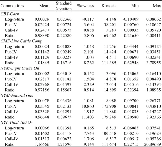
Commodity futures and options data was obtained from Thomsom-Reuters Datastream. The following commodities are included for analysis: corn, soybeans, soybean oil, wheat, live cattle, lean hogs, light crude oil, heating oil, natural gas, PJM electricity, and gold. Put and call IV’s are collected for ATM options for each contract and are also obtained from Datastream. The data period is 1/16/2008 to 7/29/2011 (T = 897 trading days). Table 1, contains summary statistics of daily log returns, put and call IV’s, and the put-call-IV ratios for selected commodities. Figures 1 through 4 display (for selected commodities) a graph of the corresponding log-return, put-IV, call-IV, and the ratio between the latter two.

3.2 Quantile Regressions Model Specifications

The general QR model from which particular specifications are to be derived is defined by equation (2.1). Given prices Pt corresponding to a NCFC, let the dependent variable

be the k-period log-return

.

As previously mentioned, the general possible predictors are the k-th lag of the

following: the own-return, the own-IV, the ratio between the put-IV and the call-IV, and factors estimated by PCA using several combinations of the complementary IVs and

(31)

Table 1. Summary Statistics (selected commodities)

Commodities Mean Standard

Deviation Skewness Kurtosis Min Max

CBT-Corn

Log-return 0.00029 0.02366 -0.117 4.148 -0.10409 0.08662

Put-IV 0.02424 0.00724 3.604 38.201 0.00760 0.10647

Call-IV 0.02477 0.00575 0.838 5.287 0.00935 0.05720

Ratio 0.98890 0.22580 5.806 69.462 0.21650 4.00411

CME-Live Cattle Comp

Log-return 0.00024 0.01088 1.048 11.256 -0.03444 0.09124

Put-IV 0.01142 0.00249 2.101 14.424 0.00671 0.03451

Call-IV 0.01129 0.00227 1.003 4.511 0.00690 0.02241

Ratio 1.01845 0.16716 8.262 111.385 0.62948 3.70955

NYM-Light Crude Oil

Log-return 0.00002 0.03018 0.152 7.096 -0.13065 0.16410 Put-IV 0.02817 0.01182 1.504 4.878 0.01352 0.08490 Call-IV 0.02968 0.01397 2.329 12.014 0.01516 0.14394 Ratio 0.97156 0.15567 0.914 14.899 0.32394 1.98935 NYM-Natural Gas Log-return -0.00078 0.03436 1.081 8.988 -0.09700 0.26771 Put-IV 0.03345 0.02133 10.860 175.908 0.00841 0.43810 Call-IV 0.03528 0.01291 1.917 11.860 0.01835 0.14227 Ratio 0.96648 0.39675 11.403 179.249 0.20580 7.92366 NYL-Gold 100 Oz Log-return 0.00066 0.01398 0.165 6.513 -0.06063 0.07541 Put-IV 0.01602 0.01118 7.743 100.518 0.00210 0.19623 Call-IV 0.01513 0.00672 1.708 6.512 0.00517 0.05268 Ratio 1.16666 1.21596 9.144 111.674 0.22715 20.89689

Figure 1. Corn: put-IV (CCCP) and call-IV (CCCC)

0 .0 2 .0 4 .0 6 .0 8 .1 C C C P 1/1/2008 7/1/2008 1/1/2009 7/1/2009 1/1/2010 7/1/2010 1/1/2011 7/1/2011 DATE .0 1 .0 2 .0 3 .0 4 .0 5 .0 6 C C C C 1/1/2008 7/1/2008 1/1/2009 7/1/2009 1/1/2010 7/1/2010 1/1/2011 7/1/2011 DATE

(32)

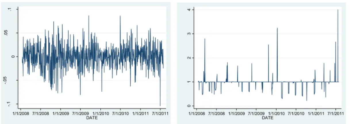
Figure 2. Corn: log-return (rCCCS) and IV-ratio (RCCC)

Figure 3. Light crude oil: put-IV (CLNCP) and call-IV (CLNCC)

Figure 4. Light crude oil: log-return (rNCLCS) and IV-ratio (RCLNCC)

-. 1 -. 0 5 0 .0 5 .1 rC C C S 1/1/2008 7/1/2008 1/1/2009 7/1/2009 1/1/2010 7/1/2010 1/1/2011 7/1/2011 DATE 0 1 2 3 4 R C C C 1/1/2008 7/1/2008 1/1/2009 7/1/2009 1/1/2010 7/1/2010 1/1/2011 7/1/2011 DATE .0 2 .0 4 .0 6 .0 8 .1 C L N C P 1/1/2008 7/1/2008 1/1/2009 7/1/2009 1/1/2010 7/1/2010 1/1/2011 7/1/2011 DATE 0 .0 5 .1 .1 5 C L N C C 1/1/2008 7/1/2008 1/1/2009 7/1/2009 1/1/2010 7/1/2010 1/1/2011 7/1/2011 DATE -. 2 -. 1 0 .1 .2 rN C LC S 1/1/2008 7/1/2008 1/1/2009 7/1/2009 1/1/2010 7/1/2010 1/1/2011 7/1/2011 DATE 0 .5 1 1. 5 2 R C LN C 1/1/2008 7/1/2008 1/1/2009 7/1/2009 1/1/2010 7/1/2010 1/1/2011 7/1/2011 DATE

(33)

returns corresponding to the rest of NCFCs. This may lead to many different arrays of relevant QR model specifications to be fitted for in-sample properties and OS

forecasting performance comparisons. The specifications described below have the same general form given by (2.1) so that different set of predictors included in the Xt

vector suffices to determine different specifications.

All of the models include an intercept (c) and a dummy variable (d) for Mondays and holidays in the vector Xt.8 The simplest model used for in-sample benchmarking is

specified by9 Model Q:

Xt-k’ = (c, d, rt-k) .

This specification can be considered an autoregressive version of QR. Then, we add own-IVs to the previous model using

Model QIV:

Xt-k’ = (c, d, rt-k, ivt-k) ,

where iv is an own-IV derived from ATM nearby put or call options. This model could be considered as the closest QRs counterpart of the Black-Scholes model. Next, we explore if relative differences between put-IVs and call-IVs could contain additional predictive information by

8_The_d_{variable is used to control for possible information differentials in markets due to distinct amounts}

of inactivity times between two consecutive trading days.

9_{Black-Scholes and GARCH models are not suitable for in-sample comparisons so that they are only}

(34)

Model QIVR:

Xt-k’ = (c, d, rt-k, ivt-k, Rt-k) ,

where Rt-k is the ratio of the put-IV to the call-IV. Up to this point, only single

commodity information has been considered. Now, other commodities IVs are incorporated using

Model QF(IV):

Xt-k’ = (c, d, rt-k, ivt-k, Rt-k, ft-k) ,

where f is a vector of top PCA-factors extracted from the rest of NCFCs put or call IVs. Similarly, the rest of NCFCs’ returns could contain forecasting information, most likely about the distribution location, via markets interactions. This is specified bt

Model QF(r):

Xt-k’ = (c, d, rt-k, ivt-k, Rt-k, frt-k) ,

where fr is a vector of top PCA-factors extracted from the rest of NCFCs log-returns. Furthermore, the combination of put and call IVs, and returns information from the rest of NCFCs could prove to be even more efficient for forecasting the return quantiles than previous models. Hence, we consider

Model QF(IV*,r):

Xt-k’ = (c, d, rt-k, ivt-k, Rt-k, fxt-k) ,

where fx is a vector of top PCA-factors obtained from pooling the rest of NCFCs IVs’ (put and call) and log-returns. Finally, we also study an augmented version of the previous model by

(35)

Model QF(IV*,r,L):

Xt-k’ = (c, d, rt-k, ivt-k, Rt-k, fzt-k) ,

where fz is a vector of top PCA-factors recovered from appending to the previous variables their corresponding first lags.

Many more specifications could be studied such as including more lags of the variables, trying other factor models, or adapting CAViaR-type specifications to our strategy. However, the OS analysis performed in this study, with the QR models sketched above, already exhausted the computer resources available for this project; therefore, such specifications are left for future research.

3.3 Quantile Regressions Estimations and In-Sample Analysis

QR models are estimated for each model combination, as outlined previously.10 This is performed in three separated blocks depending on the type of return periods, i.e., daily, weekly, and monthly. Given one type of return period, a large number of QRs have to be independently fitted.11 Hence, In order to manage the in-sample analysis, the relative frequencies of significant explanatory variables at the 5% level are determined for QR groups of particular interest via statistical software programming. In the case of PCA-factors, the relative frequency of significance (RFS here after) is referred to a Wald test about joint factors significance. Consequently, the RFS is the key measure used for most of the in-sample analysis.

10_{Details about the PCA estimation used for the QRs models are in the Appendix.}

(36)

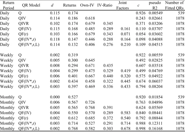
Table 2. Quantile Regressions of Log-Returns by Type of Period. Relative Frequencies of Statistical Significance (5% level) of Explanatory Variables. Combined Commodities and Quantiles.

Return

Period QR Model d Returns Own-IV IV-Ratio

Joint Factors c pseudo R2 Number of Fitted QRs Daily Q 0.115 0.174 0.926 0.00549 539 Daily QIV 0.114 0.186 0.618 0.243 0.02661 1078 Daily QIVR 0.102 0.174 0.679 0.345 0.371 0.03206 1078 Daily QF(IV) 0.115 0.168 0.485 0.289 0.161 0.110 0.03707 1078 Daily QF(r) 0.103 0.166 0.679 0.343 0.071 0.054 0.03602 1078 Daily QF(IV*,r) 0.118 0.147 0.446 0.288 0.164 0.098 0.04088 1078 Daily QF(IV*,r,L) 0.114 0.132 0.406 0.276 0.210 0.109 0.04515 1078 Weekly Q 0.002 0.319 0.922 0.00559 539 Weekly QIV 0.005 0.300 0.645 0.492 0.02825 1078 Weekly QIVR 0.008 0.294 0.671 0.435 0.607 0.03518 1078 Weekly QF(IV) 0.004 0.299 0.475 0.329 0.419 0.499 0.04769 1078 Weekly QF(r) 0.006 0.401 0.667 0.440 0.320 0.575 0.04922 1078 Weekly QF(IV*,r) 0.002 0.434 0.458 0.322 0.445 0.674 0.06037 1078 Weekly QF(IV*,r,L) 0.003 0.397 0.469 0.336 0.433 0.794 0.08204 1078 Monthly Q 0.000 0.527 0.920 0.01854 539 Monthly QIV 0.006 0.567 0.726 0.763 0.04896 1078 Monthly QIVR 0.005 0.565 0.768 0.391 0.624 0.05569 1078 Monthly QF(IV) 0.004 0.550 0.570 0.289 0.583 0.840 0.08441 1078 Monthly QF(r) 0.002 0.612 0.685 0.372 0.540 0.792 0.08844 1078 Monthly QF(IV*,r) 0.003 0.714 0.527 0.291 0.714 0.988 0.12311 1078 Monthly QF(IV*,r,L) 0.002 0.768 0.582 0.303 0.678 0.998 0.16168 1078

The analysis strategy consists of beginning with general groups of results about the QR model specifications and then breaking them down in distribution regions, and commodities. In order to obtain some return distributional information about the models RFSs, attention is focused on three regions of the density: the left and right tails, and the central area.12

12_{The quantiles considered for the left tail are 0.02, 0.04, …, and 0.24. For the right tail are 0.76, 0.78, …,}

(37)

The most general results are presented in table 2 which contains the explanatory variables’ RFSs by return period and QR model specifications. As the return period moves up from daily to weekly, and then to monthly; it is immediately clear that the RFSs become considerably higher for all of the explanatory variables (except the d variable). Regardless of return period, the models that present the highest factors’ RFSs tend to be those that pool IVs with returns. This is probably an indication that

information about distribution location and scale is better conveyed in this way. Focusing on the own-IVs, in general, they tend to have the highest RFS among all explanatory variables, an expected result since this resembles the Black-Scholes model. The RFSs become slightly lower; however, when factors are included in the models, suggesting that the information in other markets, summarized in factors, contains supplementary explanatory power. Another important fact is that the factor’ RFSs start lower than the own-IVs’ RFSs and the IV-ratios’ RFSs for daily returns; but then, they become stronger as the return period is higher. In fact, for monthly returns, the factors RFSs end up actually higher than own IVs’ and IV-ratios’ RFSs. A similar behavior can be observed about the own-returns. Finally, the IV ratios have higher RFSs when

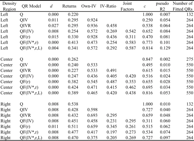
combined with factors for all return periods maintaining similar levels among them. Tables 3, 4, and 5 are very similar to table 2 but, in addition, they show the distribution regions for daily, weekly, and monthly returns respectively. As can be observed, table 3 shows that factors’ RFSs are stronger in the tails than in the center. More precisely, factors’ RFSs are highest in the left tail, followed by the right tail, and lowest in the center. However, this pattern changes in table 4 (weekly) and 5 (monthly).

(38)

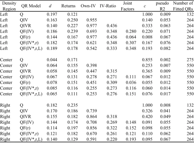
Table 3. Quantile Regressions of Daily Returns by Density Region. Relative Frequencies of Statistical Significance (5% level) of Explanatory Variables. Combined Commodities and Quantiles.

Density

Region QR Model d Returns Own-IV IV-Ratio

Joint Factors c pseudo R2 Number of Fitted QRs Left Q 0.197 0.121 1.000 0.009 132 Left QIV 0.163 0.250 0.955 0.140 0.053 264 Left QIVR 0.140 0.227 0.977 0.436 0.333 0.063 264 Left QF(IV) 0.186 0.239 0.693 0.348 0.280 0.220 0.071 264 Left QF(r) 0.144 0.167 0.977 0.436 0.064 0.008 0.067 264 Left QF(IV*,r) 0.182 0.174 0.621 0.348 0.307 0.167 0.076 264 Left QF(IV*,r,L) 0.189 0.178 0.542 0.333 0.348 0.193 0.082 264 Center Q 0.044 0.171 0.855 0.002 275 Center QIV 0.064 0.155 0.398 0.253 0.007 550 Center QIVR 0.058 0.145 0.447 0.315 0.365 0.009 550 Center QF(IV) 0.067 0.131 0.278 0.271 0.111 0.067 0.012 550 Center QF(r) 0.078 0.151 0.451 0.309 0.036 0.055 0.012 550 Center QF(IV*,r) 0.085 0.116 0.255 0.273 0.116 0.060 0.014 550 Center QF(IV*,r,L) 0.065 0.111 0.253 0.276 0.151 0.076 0.017 550 Right Q 0.182 0.235 1.000 0.008 132 Right QIV 0.170 0.186 0.739 0.326 0.041 264 Right QIVR 0.155 0.182 0.864 0.318 0.420 0.049 264 Right QF(IV) 0.144 0.174 0.708 0.269 0.148 0.091 0.055 264 Right QF(r) 0.114 0.197 0.856 0.322 0.152 0.098 0.055 264 Right QF(IV*,r) 0.121 0.182 0.670 0.261 0.121 0.110 0.062 264 Right QF(IV*,r,L) 0.140 0.129 0.591 0.220 0.193 0.095 0.067 264

In table 4, the factors’ RFSs corresponding to the center become higher than the right tail, with the left tail still leading the RFSs levels. Table 5, suggests that skewness shape varies with the return period. Regarding the own-IVs’ RFSs (see table 3), they are much stronger in the tails than in the center. These results are expected since the own-IV’s represent the market’s expectations about future volatility (second moment) and can be considered further evidence that IVs are good predictors of realized volatility.

(39)

Table 4. Quantile Regressions of Weekly Returns by Density Region. Relative

Frequencies of Statistical Significance (5% level) of Explanatory Variables. Combined Commodities and Quantiles.

Density

Furthermore, notice that for models that do not include factors, most own-IVs’ RFSs in the tails are very high (more than 0.90) which; on one hand, reinforces the previous comment; on the other hand, it may be an indication that the inclusion of factors in the QR models provides important predictive information that causes own-IVs’ RFSs to become lower.

(40)

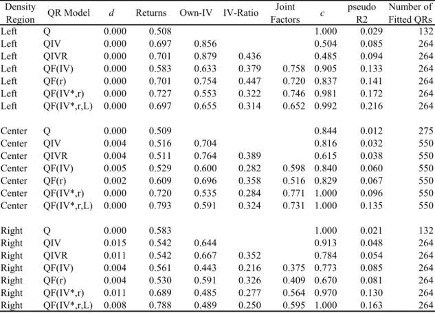
Table 5. Quantile Regressions of Monthly Returns by Density Region. Relative

Frequencies of Statistical Significance (5% level) of Explanatory Variables. Combined Commodities and Quantiles.

Density

In table 4 (weekly), the results about own-IVs still show similar behavior to table 3 (daily) , but in table 5 (monthly), they change in a puzzling way. First, as was stated earlier, for models that include factors, their RFSs completely dominate not only the own-IVs’ RFSs but also they become the strongest predictors of all. And second, for models that do not include factors, the own-IVs’ RFSs are now strongest in the left tail, followed by the center, and then by the right tail. This could be interpreted as factors taking over much of the tail distribution prediction ability for monthly returns, probably

(41)

as a result of IVs best reflecting shorter horizons expectations of volatility. Regarding the IV-ratios, in addition to what was stated previously, their RFSs are lowest in the right tail and about the same on the center and left; pattern that is maintained for all horizons.

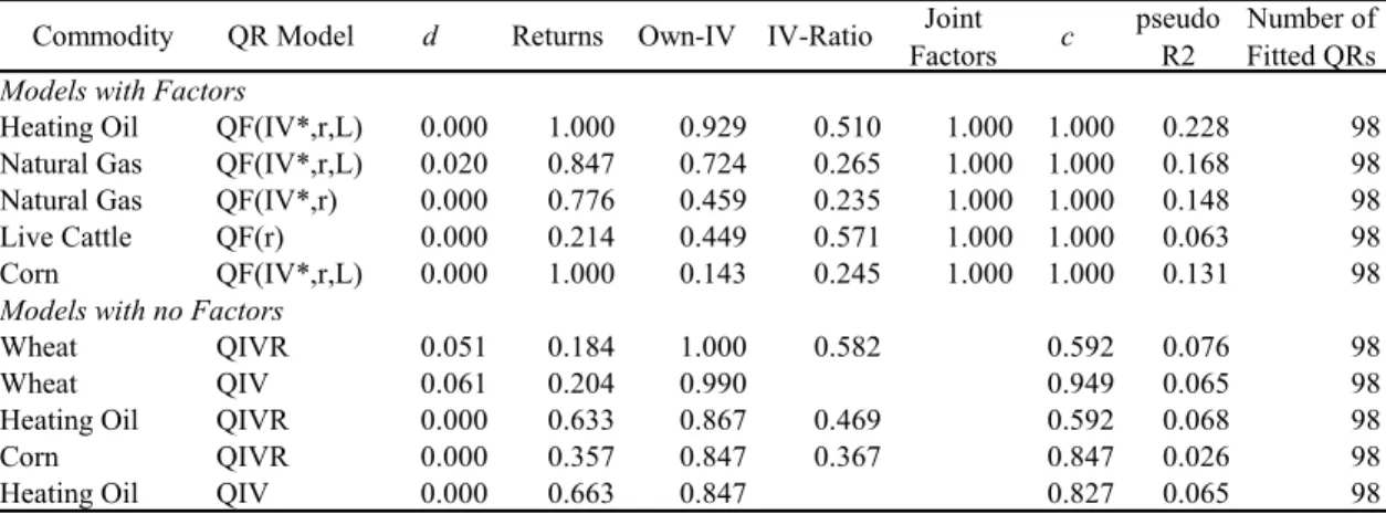
Table 6. Quantile Regressions of Daily Returns. Relative Frequencies of Statistical Significance (5% level) of Explanatory Variables. Top Commodities and Models Specifications.

Commodity QR Model d Returns Own-IV IV-Ratio Joint

Factors c

pseudo R2

Number of Fitted QRs Models with Factors

Heating Oil QF(IV*,r,L) 0.000 0.020 0.561 0.561 0.684 0.469 0.057 98

Heating Oil QF(IV*,r) 0.000 0.020 0.459 0.510 0.673 0.357 0.050 98

Heating Oil QF(IV) 0.000 0.061 0.469 0.388 0.469 0.367 0.046 98

Soybeans QF(r) 0.133 0.276 0.786 0.235 0.378 0.286 0.037 98

Gold QF(IV*,r,L) 0.000 0.051 0.480 0.143 0.357 0.061 0.056 98

Models with no Factors

Light Crude Oil QIV 0.000 0.214 0.847 0.051 0.061 98

Light Crude Oil QIVR 0.000 0.173 0.847 0.173 0.163 0.064 98

Soybeans QIVR 0.112 0.153 0.827 0.276 0.194 0.031 98

Gold QIVR 0.000 0.143 0.816 0.388 0.663 0.043 98

Heating Oil QIVR 0.010 0.031 0.816 0.408 0.418 0.038 98

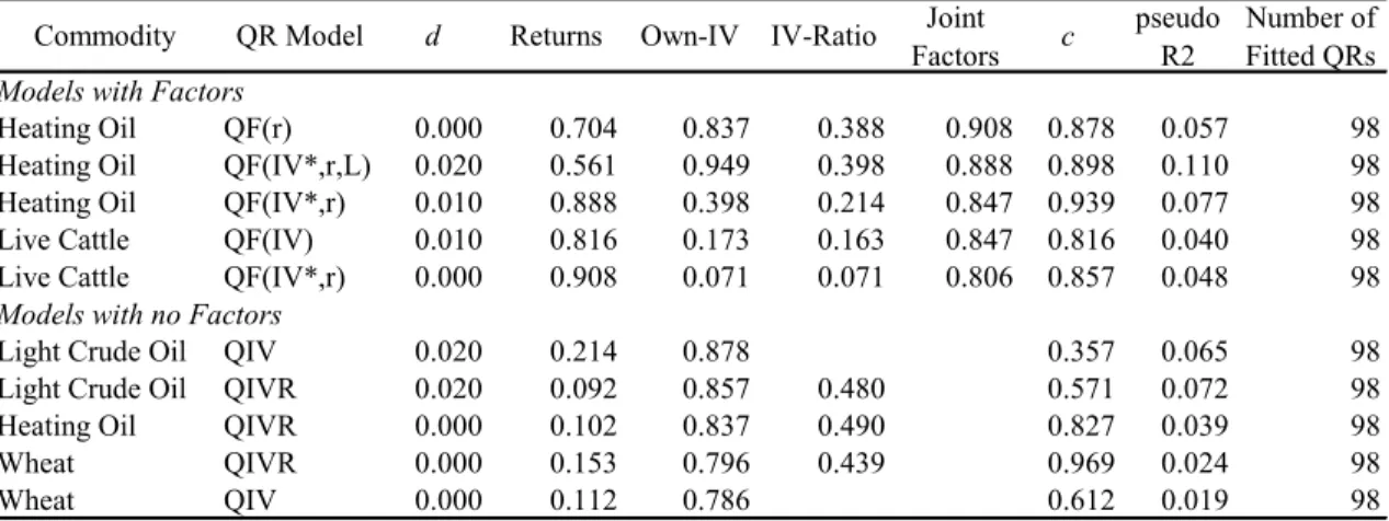
Table 7. Quantile Regressions of Weekly Returns. Relative Frequencies of Statistical Significance (5% level) of Explanatory Variables. Top Commodities and Models Specifications.

Factors c

pseudo R2

Heating Oil QF(r) 0.000 0.704 0.837 0.388 0.908 0.878 0.057 98

Heating Oil QF(IV*,r) 0.010 0.888 0.398 0.214 0.847 0.939 0.077 98

Live Cattle QF(IV) 0.010 0.816 0.173 0.163 0.847 0.816 0.040 98

Live Cattle QF(IV*,r) 0.000 0.908 0.071 0.071 0.806 0.857 0.048 98

Light Crude Oil QIV 0.020 0.214 0.878 0.357 0.065 98

Light Crude Oil QIVR 0.020 0.092 0.857 0.480 0.571 0.072 98

Heating Oil QIVR 0.000 0.102 0.837 0.490 0.827 0.039 98

Wheat QIVR 0.000 0.153 0.796 0.439 0.969 0.024 98

(42)

Table 8. Quantile Regressions of Montly Returns. Relative Frequencies of Statistical Significance (5% level) of Explanatory Variables. Top Commodities and Models Specifications.

Factors c

pseudo R2

Natural Gas QF(IV*,r,L) 0.020 0.847 0.724 0.265 1.000 1.000 0.168 98

Natural Gas QF(IV*,r) 0.000 0.776 0.459 0.235 1.000 1.000 0.148 98

Live Cattle QF(r) 0.000 0.214 0.449 0.571 1.000 1.000 0.063 98

Corn QF(IV*,r,L) 0.000 1.000 0.143 0.245 1.000 1.000 0.131 98

Wheat QIVR 0.051 0.184 1.000 0.582 0.592 0.076 98

Wheat QIV 0.061 0.204 0.990 0.949 0.065 98

Heating Oil QIVR 0.000 0.633 0.867 0.469 0.592 0.068 98

Corn QIVR 0.000 0.357 0.847 0.367 0.847 0.026 98

Heating Oil QIV 0.000 0.663 0.847 0.827 0.065 98

Table 6, 7, and 8 (daily, weekly, and monthly returns) present the 5-top NCFC-models combinations with factors (sorted from largest to smallest factors’ RFSs) and the 5-top NCFC-models with no factors (sorted from largest to smallest by own-IVs’

RFSs).13 Hence, now we can examine which NCFCs correspond to the top models (by RFSs particular variables). Notice the very high values of most RFSs. Merging all return periods for models with factors; heating oil, natural gas, live cattle, soybean, gold, and corn comprise the highest factors’ RFSs. Analogously, for models with no factors, light crude oil, heating oil, wheat, gold, corn, and live cattle present the greatest own-IVs’ RFSs.

In summary, the previous in sample analyses presents evidence that PCA-factors that pool IVs (put and call) with returns used as QR’s predictors are likely to provide an

(43)

important contribution for forecasting the conditional return distribution of some

NCFCs, in addition to the own-IVs, IV-ratios, and own-returns. It was also observed that the own-returns RFSs increased considerably for returns with longer horizons. However, it is difficult to establish, with in-sample analysis which of the QR-models, here

specified, are actually the best for quantile forecasting purposes. This issue is often elucidated using out-of sample performance analysis.

3.4 Out-of-Sample Quantile Forecasting Performance

3.4.1. Out-of Sample Hit Percentage Deviations and the Dynamic Quantile Test The recursive forecasting method described above (section 2.2.3.2) was applied to the numerous QR models specifications using the last 200 out of the 897 observations. Accordingly, the Hit% (2.10) and the DQ test-statistics (2.11) were obtained for the previously considered QR model specifications; and now, for the Black-Scholes quantile forecasts obtained by equation (2.6); and the n-GARCH and t-GARCH quantile forecast generated using equations (2.8) and (2.9) respectively. Similar to al QR models that include own-IVs (QIV, QIVR, and QFs); notice that the Black-Scholes quantile forecasts and their corresponding Hit% indices as well as the DQ statistics are generated for as many as 1078 items (11 commodities 2 IV-types 49 quantiles). Having this large number of Hit% indices and DQ statistics requires a similar examination strategy to the in-sample analysis.

(44)

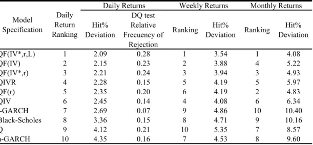
Table 9. Out-of-Sample Performance of Quantile Regressions, Black-Scholes, and GARCH models. Hit% Deviations and Dynamic Quantile Test Relative Frequency of Rejection. By Model Specification and Type of Own-Implied Volatility.

Hit% Deviation DQ test Relative Frecuency of Rejection Ranking Hit% Deviation Ranking Hit% Deviation QF(IV*,r,L) 1 2.09 0.28 1 3.54 1 4.08 QF(IV) 2 2.15 0.23 2 3.88 4 5.22 QF(IV*,r) 3 2.21 0.24 3 3.94 3 4.93 QIVR 4 2.28 0.15 5 4.19 5 5.97 QF(r) 5 2.35 0.20 6 4.19 2 4.83 QIV 6 2.45 0.14 4 4.08 6 6.34 t-GARCH 7 2.69 0.07 9 4.86 10 10.40 Black-Scholes 8 3.36 0.15 8 4.71 9 10.16 Q 9 4.12 0.21 10 5.35 7 8.57 n-GARCH 10 4.35 0.16 7 4.53 8 9.60 Daily Returns Model Specification Daily Return Ranking

Weekly Returns Monthly Returns

Table 9 presents the most aggregated results. Notice that there are three groups of two columns, each group belonging to daily, weekly, and monthly returns. For daily returns, the first column, titled “Hit% Deviations” (HD), shows the average of the absolute difference (in percent points) between the Hit% index and 100q.14 The lower the HD is, the better the unconditional quantile forecasting coverage correctness. For daily returns, the second column contains the relative frequencies that the DQ tests were rejected (DQR). Since the null hypothesis is that the hits are independent, the lower the DQR is, the less autocorrelated are the hits.

Based on the daily HDs, the top two models are three models are QF(IV*,r,L), QF(IV), and QF(IV*,r). Notice that the best model is the one that pooled the

complementary IVs (put and call) with complementary returns and their first lag for

(45)

obtaining the PCA-factors. Interestingly, for weekly and monthly returns this model is also the best. However, its DQR is also the worst (.28). Yet this number by itself does not look very high since it also means that in 72% of occurrences the corresponding individual QRs models were not rejected by the DQ test. Remarkably, notice that the top three models include factors as predictors, whereas the worst performers tend to be GARCH and Black-Scholes models. This pattern is fairly stable for weekly and monthly returns at this level of aggregation. Furthermore, observe that Black-Scholes and

GARCH models, being the worst ones according to HD, have among the lowest DQRs. This suggests that, combining models may be an important direction for future research, in addition to including more lags of the explanatory variables in QRs. Finally, all of the top five models include the IV-ratio which is a strong indication that differences from put-IVs and call-IVs are quite relevant in forecasting the returns distribution.

Apparently, the weekly and monthly HDs appear to be deceptively greater than daily HDs. However this comparison is not straight forward at all. One aspect that could interfere is that weekly and monthly returns standard deviations are considerably higher than daily. Although the IVs forecasted standard deviations were carefully rescaled to the number of return periods considered, the agents’ horizon expectations may make a difference. A more clear reason is that when large unexpected jumps occur (IVs would not reflect it until they realize or are closed to it), forecasted k-period returns will maintain large and correlated forecast errors for nearly k periods until the innovation become real data and models correct for it. The situation is analogous for density forecast that will be failing to correctly cover realizations for a while. Forecasting a

(46)

monthly return is equivalent to forecast the price level a month from present time which is much more difficult than forecasting the one-day-ahead price. The higher monthly and weekly HDs might actually be relatively lower than the daily ones considering that the HD increase may be less than the climb in forecasting difficulty.

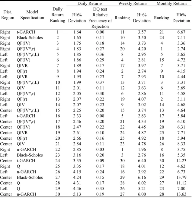
Table 10. Out-of-Sample Performance of Quantile Regressions, Black-Scholes, and GARCH. Hit% Deviations and Dynamic Quantile Test Relative Frequency of Rejection. By Distribution Region, Model Specification, and Type of Own-Implied Volatility.

Hit% Deviation DQ test Relative Frecuency of Rejection Ranking Hit% Deviation Ranking Hit% Deviation Right t-GARCH 1 1.64 0.00 11 3.57 21 6.67 Right Black-Scholes 2 1.65 0.11 10 3.50 24 7.11 Right QF(IV) 3 1.75 0.18 14 3.73 4 3.36 Right QF(IV*,r) 4 1.83 0.27 20 4.20 1 2.74 Left QF(IV*,r,L) 5 1.85 0.36 8 2.95 5 3.65 Left QF(IV) 6 1.86 0.29 4 2.81 15 4.72 Right QIVR 7 1.89 0.17 17 3.97 7 3.71 Left QF(r) 8 1.94 0.24 2 2.74 9 4.15 Left QIVR 9 1.95 0.23 7 2.93 10 4.44 Right QF(IV*,r,L) 10 1.99 0.37 13 3.71 3 3.31 Right QIV 11 2.01 0.11 12 3.63 6 3.69 Left QF(IV*,r) 12 2.05 0.30 6 2.86 11 4.58 Right QF(r) 13 2.07 0.22 19 4.07 2 3.11 Left QIV 14 2.07 0.23 9 3.02 14 4.68 Center QF(IV*,r,L) 15 2.25 0.20 15 3.74 13 4.64 Left t-GARCH 16 2.33 0.08 5 2.83 17 5.84 Center QF(IV*,r) 17 2.46 0.20 21 4.33 19 6.10 Center QF(IV) 18 2.47 0.22 22 4.45 20 6.31 Center QIVR 19 2.61 0.10 24 4.87 25 7.71 Center QF(r) 20 2.66 0.16 25 4.92 18 5.94 Center QIV 21 2.84 0.11 23 4.78 26 8.33 Right n-GARCH 22 2.85 0.03 1 1.96 8 3.75 Left Black-Scholes 23 3.16 0.20 3 2.76 16 5.35 Center t-GARCH 24 3.35 0.09 30 6.40 30 14.23 Right Q 25 3.35 0.17 18 4.01 12 4.62 Left n-GARCH 26 4.15 0.24 16 3.92 22 6.73 Center Black-Scholes 27 4.24 0.15 29 6.16 29 13.79 Center Q 28 4.31 0.17 28 6.02 27 11.12 Left Q 29 4.46 0.35 26 5.21 23 7.00 Center n-GARCH 30 5.13 0.19 27 6.00 28 13.63 Monthly Returns Dist. Region Model Specification Daily Return Ranking

(47)

Table 10 is very similar to table 9 but the models are broken down by

distributions regions. The most outstanding fact is that all of the region-models ranked above the 15th position corresponds to the tails (there are 30 possible items). Although the top region-model is right-t-GARCH, this model is also a poor performer for the center and left distributions regions, ranked 24th and 16th respectively. An even more extreme behavior is shown by the second best (right-Black-Scholes) which is ranked 27th and 23th for the center and left regions respectively. Notice that these models are based on log-returns symmetric distributions; therefore, their poor performance in one of the tails is evidence of excess skewness. Finally, although the rankings changed for weekly and monthly returns, the previous findings still hold up to some extent. For example, on a weekly basis, the t-GARCH model is ranked 5th in the left, 30th in the center, and 11th on the right.

Table 11 is analogous to tables 9 and 10 except that now the models are grouped by NCFCs. The table contains the top 30 items (out of 110) by daily HD. This table allows to identify, among the top items, those with the serial correlation problems. For example, the best model on the average was, according to table 9, the QF(IV*,r,L) specification; but, it had a high DQR. Now we can see that the greatest DQR belongs to light crude oil (0.60) followed by wheat (0.56), and soybeans (0.30). Notice that the top daily HD item is corn t-GARCH (1.10 HD and 0.04 DQR). However, this is not the best model when other return periods are considered. The actual lowest HD is 1.02

corresponding to lean hogs QF(IV*,r). We let the readers finding other near top items by weekly or monthly HD that performe better than others daily HD items in this list.

(48)

Table 11. Out-of-Sample Performance of Quantile Regressions, Black-Scholes, and GARCH models. Hit% Deviations and Dynamic Quantile Test Relative Frequency of Rejection. By Commodity Future Contract and Model Specification.

Hit% Deviation DQ test Relative Frecuency of Rejection Ranking Hit% Deviation Ranking Hit% Deviation Corn t-GARCH 1 1.10 0.04 35 2.82 77 8.81 Corn QIV 2 1.12 0.06 10 1.80 18 3.45 Corn QF(IV) 3 1.15 0.08 3 1.40 19 3.47 Wheat t-GARCH 4 1.17 0.08 7 1.68 35 4.92 Corn Q 5 1.32 0.08 2 1.32 33 4.51 Corn QF(r) 6 1.36 0.04 22 2.36 25 3.88 Wheat Q 7 1.41 0.24 16 2.11 42 5.54

Lean Hogs QF(IV) 8 1.42 0.10 32 2.77 56 6.62

Lean Hogs QF(IV*,r,L) 9 1.47 0.04 4 1.47 65 7.45

Lean Hogs QIVR 10 1.50 0.02 85 5.70 86 9.62

Corn QIVR 11 1.51 0.06 20 2.29 16 3.44

Soybeans QF(IV) 12 1.53 0.32 37 2.92 13 2.86

Soybeans QF(IV*,r) 13 1.56 0.32 25 2.55 29 4.12

Wheat Black-Scholes 14 1.57 0.08 9 1.76 34 4.65

Natural Gas QF(IV*,r,L) 15 1.57 0.18 87 5.82 60 6.83

Natural Gas QF(IV) 16 1.61 0.08 93 6.28 90 10.06

Soybeans QF(IV*,r,L) 17 1.64 0.30 34 2.81 30 4.22

Natural Gas QF(IV*,r) 18 1.66 0.10 91 6.24 53 6.41

Lean Hogs QF(IV*,r) 19 1.66 0.08 1 1.02 44 5.71

Wheat QF(IV*,r,L) 20 1.67 0.56 14 2.04 5 1.92

Wheat QF(IV) 21 1.67 0.40 31 2.73 10 2.46

Lean Hogs QIV 22 1.67 0.00 90 5.99 83 9.48

Light Crude Oil QF(IV*,r,L) 23 1.70 0.60 18 2.21 9 2.43

Light Crude Oil QIV 24 1.73 0.10 5 1.53 20 3.59

Soybeans QIVR 25 1.74 0.32 38 2.97 28 4.07 Corn QF(IV*,r,L) 26 1.77 0.12 23 2.47 2 1.56 Corn QF(IV*,r) 27 1.78 0.10 12 1.85 12 2.76 Lean Hogs QF(r) 28 1.81 0.04 81 5.33 74 8.16 Live Cattle Q 29 1.83 0.16 41 3.22 72 7.91 Corn n-GARCH 30 1.83 0.04 39 3.15 73 8.03

Daily Returns Weekly Returns Monthly Returns Nearby Commodity Future Contract Model Specification Daily Return Ranking

In general, the evidence can be considered strong and robust that factors can contribute with additional quantile forecasting power to the individual commodities IVs information. It seems also important that the ratios of the put-IV to the call-IV can contribute to improving the log-returns quantile forecasting performance, in addition to