Effect size estimation and robust classification for irregularly sampled functional data

(1)

c

(2)

EFFECT SIZE ESTIMATION AND ROBUST CLASSIFICATION FOR IRREGULARLY SAMPLED FUNCTIONAL DATA

BY

YEONJOO PARK

DISSERTATION

Submitted in partial fulfillment of the requirements for the degree of Doctor of Philosophy in Statistics

in the Graduate College of the

University of Illinois at Urbana-Champaign, 2017

Urbana, Illinois

Doctoral Committee:

Professor Douglas Simpson, Chair Professor Jeffrey Douglas

Associate Professor Feng Liang Professor Xiaofeng Shao

(3)

Abstract

Functional data arise frequently in numerous scientific fields with the development of modern technology. Accordingly, functional data analysis to extract information on curves or functions is an important area for investigation. In this thesis, we address two key issues: measuring an effect size of variable of the interest in functional analysis of variance (fANOVA) model and the development of robust probabilistic classifier in functional response model. We especially consider irregular functional data in our study, where curves are collected over varying or non-overlapping intervals.

First, we develop an approach to quantify the effect size on functional data, per-form functional ANOVA hypothesis test, and conduct power analysis. We develop an approach to quantify the effect size on functional data, perform functional ANOVA hypothesis test, and conduct power analysis. We introduce the functional signal-to-noise ratio (f SN R), visualize the magnitude of effects over the interval of interest, and perform bootstrapped inferences. It can be applicable when the individual curves are sampled at irregularly spaced points or collected over varying intervals. The pro-posed methods are applied in the analysis of functional data from inter-laboratory quantitative ultrasound measurements, and in a reanalysis of Canadian weather data. Moreover, we represent the asymptotic power of functional ANOVA test as a function of proposed measure. The agreement between the asymptotic and empirical results is examined and found to be quite good even for small sample sizes. The asymptotic lower bound of power can be reasonably used to determine sample size in planning

(4)

experimental design.

Secondly, we build a robust probabilistic classifier for functional data, which pre-dicts the membership for given input as well as provides informative posterior prob-ability distribution over a set of classes. This method combines Bayes formula and semiparametric mixed effects model with robust tuning parameter. We aim to make the method robust to outlying curves especially in providing robust degree of certainty in prediction, which is crucial in medical diagnosis. It can be applicable to various practical structures, such as unequally and sparsely collected samples or repeatedly measured curves retaining between-curve correlation, with very flexible spatial co-variance function. As an illustration we conduct simulation studies to investigate the sensitivity behaviors of probability estimates to outlying curves under Gaussian assumption and compare our proposed classifier with other functional classification approaches. The performance is evaluated by imposing more penalty for being con-fident but false prediction. The value of the proposed approach hinges on its simple, flexible, and computational efficiency. We illustrate the issues and methodology in ultrasound quantitative ultrasound, backscatter coefficient vs. frequency functional data, commonly obtained as irregular form and public dataset with artificial contam-ination. We also show how to implement proposed classifier in R.

(5)

This dissertation is dedicated to

my parents, for yours steadfast support and love, and my husband, for being an amazing partner and friend

(6)

List of Figures

1.1 Backscatter functions for one of the scanned tumors . . . 3 2.1 Approximated (“A”) and simulated (“S”) power curves as a function

of effect size on each scenario. . . 31 2.2 Power functions under d = 0.1, 0.4 and 0.9 for (a) Gf SN R = 0.2, (b)

Gf SN R= 0.4 and (c) Gf SN R = 0.8 . . . 32

2.3 (Top) Pointwise estimate of the difference in magnitude of the BSC es-timates between two tumors, noise error, and random effect for ‘setup’ from pointwise mixed ANOVA. (Bottom) pointwise tumor effect and marginal error from pointwise 1-way ANOVA . . . 32 2.4 Transducer L14-5. (a) The average and SD curves of 4T1 and MAT,

(b) Pointwise and smoothed f SN R . . . 33 2.5 The smoothedf SN R and bootstrapped 90 % confidence intervals . . 33 2.6 The smoothed f SN R and bootstrapped 90% confidence intervals of

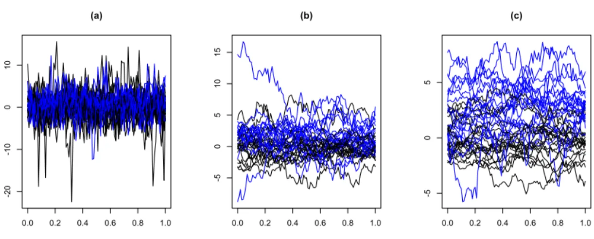
(a) Temperature and (b) Precipitation . . . 34 3.1 Illustration of heavy-tailed sample curves under different magnitudes

of within-curve dependency. (a) weak (b) moderate (c) strong. . . 65 3.2 Posterior probabilities from RSMM and GSMM. Red dots denote

mis-classifiction rates . . . 66 3.3 Test error (left) and LogLoss (right) under weak (top), moderate

(mid-dle), strong (bottom) within-curve dependency structure . . . 67 3.4 Test error and LogLoss under sparse data . . . 68 3.5 Test error and LogLoss under Cauchy (top), t distribution with 5 df

(middle) and Gaussian simulated data with different robust tuning parameter ν . . . 69 3.6 Phantom data. A1A2. . . 70 3.7 A sample of 10 contaminated log-periodograms within each phoneme

class. 5 black curves on frequency [1 : 128] and 5 green curves on frequency [129 : 256] . . . 71 3.8 Test error and LogLoss in contaminated phoneme example from 50

(9)

List of Tables

2.1 Simulation 1: approximated and empirical sizes and powers of the

F- and F∗_{-test under stationary process model (G} ₌ _G

f SN R, G∗ =

G∗_{f SN R}) . . . 35 2.2 Simulation 2: approximated and empirical sizes and powers of F- and

F∗_{-test under the model with cyclic marginal error function} _{. . . . .} ₃₆

2.3 Simulation 3: approximated and empirical sizes and powers of F- and

F∗_{-test under heteroscedisticity model} _{. . . .} ₃₆

F∗_{-test under the model with non-parallel mean functions} _{. . . .} ₃₇

F∗_{-test under non-stationary process model} _{. . . .} ₃₇

2.6 Estimates of tumor effect size (bootstrappedp-values in parentheses) 38 2.7 Tumor type effect size for each transducer . . . 38 2.8 Transducer effect size for each tumor type and frequency range . . . . 38 2.9 The regional effect size for the Canadian daily temperature and

pre-cipitation data (with bootstrap p-values in parentheses) . . . 39 3.1 Test error and LogLoss under moderate within-curve dependency . . 73 3.2 Test error and LogLoss under Gaussian data . . . 73 3.3 leave-one-out cv error and LogLoss for phantom A1A2 data. . . 73 3.4 10-fold cross validated error and LogLoss for mammary data . . . 73 3.5 Mean test errors and LogLoss for contaminated (original) phoneme

(10)

Chapter 1 Introduction

With continual developments in instrumentation and advanced computing, there has been an increasing need for modeling and analyzing functional data that are col-lected nearly continuously over fine grids or regions of interest. In accordance with this growth, there is an extensive literature on methods for functional data analysis (Ramsay and Silverman, 2005). Less well developed, to our knowledge, are studies on irregularly sampled curves which are collected on varying or non-overlapped intervals. Our studies focus on the analysis of irregularly sampled functional data, especially the estimation of effect size to quantify the magnitude of the relationship between functional response and variable of interest in fANOVA and construction of robust classifier providing degree of certainty for diagnosis purpose.

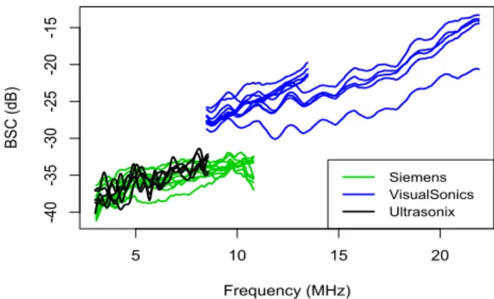
This research is motivated by quantitative ultrasound (QUS) data which aim to extract diagnostically useful information from the ultrasound radio frequency sig-nals, in particular the backscatter (BSC) and attenuation properties of the scanned material along different scan lines (Wirtzfeld et al., 2013). Wirtzfeld et al. (2015) presented data and results from diagnostic ultrasound studies using multiple trans-ducers to scan mammary tumors and fibroadenomas (benign fibrous masses) in rats and mice. The frequency dependent BSC curves derived from the power spectra of these scans took the form of functional measurements spanning the frequency range of the ultrasound transducer.

(11)

widely used in medical applications. However, for BSC measurements to translate to the clinic, the detection of differences in the features of the BSC curves for different tumors needs to be statistically assessed. Beyond statistical inference, variation due to tumor effect needs to be compared with variation due to background noise to study the precision in diagnosis. In such settings it is worth examining tumor effect sizes on BSC curves both locally and globally. For example, clinicians might be interested in the overall effect size over the frequency range of interest to make sure about the precision in diagnosis, otherwise, the pointwise effect size evaluated at each grid is of interest for researchers to develop the measurement system achieving the most effective separation. Furthermore, by examining confidence intervals of local effect size, we can infer whether the change of effect size over frequencies is statistically significant or not.

As a next stage, if statistically distinct behaviors in BSC functions over different types of tumor are proved, then an immediate question we may have correspondingly is, whether the functional data classification method can diagnose the future obser-vations into the correct classes. Especially providing stable and informative posterior probabilities to be assigned to each class is of interest in terms of diagnostic purpose. However motivating data has a challenging structure as in Figure 1.1. It is irregu-larly collected over frequencies, seemingly heavy-tail distributed with large noise and has dependence structure between multiple curves. In experiment, functional BSC are collected in several laboratories using different transducers covering different ranges of frequency, scanning the target tumor in living animal multiple times. Thus curves retaining between-curve correlation have varying grid points and intervals. In addi-tion, noninvasive scan causes potential outlying behaviors suffered from unexpected contamination by scanning neighboring other tissues or noise in environment.

(12)

5 10 15 20 -4 0 -3 5 -3 0 -2 5 -2 0 -1 5 Frequency (MHz) BSC (d B) Siemens VisualSonics Ultrasonix

Figure 1.1: Backscatter functions for one of the scanned tumors

local effect size along the entire functional domain. It provides not only graphical visualization but also valuable information about which ranges have the largest effect size. Secondly, we define a globalized effect size that summarizes effect size over region of interest. Third, we represent the asymptotic power of fANOVA test as a function of proposed global measure. The agreement between the asymptotic and empirical results is examined via simulation studies under different scenarios and found to be quite good even for small sample sizes. This agreement and asymptotic lower bound of power enable to derive sample size estimation tool for planning experimental design. In Chapter 3, we build a robust probabilistic classifier for functional grouped data, which provides a predicted class label as well as a probability distribution over a set of classes. It is based on spline based mixed-model with robust tuning parameter and Bayes rule, and especially mixed effects model approach enables to approximate covariance function in a flexible and efficient way. The key of our method is to impose heavy-tail distribution assumption with robustness parameter ν on random coefficients to yield robust result. We focus on the evaluation of functional data classifier in terms of accuracy for predicted posterior probability to be assigned to the

(13)

correct class.

In Chapter 4, we sketch the foundation of asymptotic analysis for unbalanced functional data, for large sample inference and theoretic basis for use of the bootstrap.

(14)

Chapter 2 Effect Size and Power Analysis for

Functional ANOVA

2.1 Introduction

Functional data in which the response measurements consist of functions observed continuously over a fine grid occur in many different fields more often in recent years. In accordance with this growth, there is an extensive literature on methods for functional data analysis. Ramsay and Silverman (2005) provide a comprehensive treatment. Also a number of authors have developed global testing and inference for k-group functional response data including the functional analysis of variance (fANOVA) methods of Cuevas et al. (2004), Shen and Faraway (2004), and Zhang and Liang (2014).

Less well developed, to our knowledge, are studies on the estimation of effect size to quantify the magnitude of the relationship between functional response and vari-able of interest. Indeed, characterizing an effect size is prominent in practical studies, because research findings can be clearly presented by this measure. It also facilities interpretation and performs a fair comparison among variables due to its robustness in scale and measurement units. Additionally, effect size is closely related to statis-tical power of a hypothesis test, which can be used for sample size determination in experimental design or for interpretation of test result.

In related work Yao, Muller and Wang (2005a) proposed the coefficient of deter-mination in functional linear regression to define a global measure of the association.

(15)

They proposed two types of functionalR2 _{by integrating the pointwise}_R2₍_s_{) over the}

domain s and by integrating the numerator and the denominator separately. Those measures estimate global effect size overs, however, further statistical inference based on them was not concerned. PartialR2 _{proposed by Edwards}_{et al.} _{(2008) measures}

such magnitude in mixed effect structure, especially for the longitudinal linear mixed model. However, some restrictive parametric assumptions are required and the con-nection between an effect size and statistical inference received less attention in the study.

We propose a general approach to estimate the effect size of the variable of interest and further analysis for the functional data. While many developed methodologies are restricted to regular structure where curves are collected over common grids and interval, our proposed analysis can be applicable to irregular structure where collec-tions of curves are unequally and sparsely sampled over varying intervals. In this paper, the measures quantifying local and global effects of the variable are developed. A key idea is to extend the signal-to-noise ratio (SN R), a widely used measure in engineering defined as the ratio of the variance of the target signal to the variance of noise, to functional structure. Indeed, closely related concepts have developed in the statistics literature as well, for example, noncentrality parameter of theF-statistic in ANOVA. It is often used as a measure of effect size or as a planning tool in power analysis. The extensions developed in the present paper are designed to provide anal-ogous types of analysis for functional response data. Specifically, the use of estimated global measure as an inferential statistic to detect significant effect over the domain is studied. We discuss the use of the proposed local measure for visualization and derivation of confidence intervals to find which parts of the function domain are most informative.

(16)

with little attention paid to power analysis under finite-sample. Although Zhang (2011) and Zhang and Liang (2014) studied asymptotic powers of functional F-type tests in fANOVA model, the main goal was to show root-n consistency of tests. Shen and Faraway (2004) estimated power and size of test via simulation studies, but the purpose was to compare existing test methods. In this paper, we represent asymptotically approximated statistical power as a function of proposed effect size and study the agreement between the asymptotic and empirical powers under finite sample sizes. We also derive asymptotic lower bounds of the power of fANOVA tests based on the proposed effect size. The accuracy of the asymptotic approximation is found to be good for moderate sample sizes, which implies approximated lower bounds can be used for sample size determination. It enables sample size estimation in the design of experiment.

The rest of the paper is organized as follows. In Section 2, we introduce the functional SN R to measure the local effect size and extend it to fANOVA model. We define global measure over the interval of interest and present estimation of pro-posed measures. Also statistical inferences based on local and global effect sizes are introduced. In Section 3, the agreement between the asymptotic and empirical pow-ers under finite sample size are investigated on various scenarios. Also it provides asymptotic approximation of lower bounds of power as a tool for sample size deter-mination and its numerical implementation. We return to quantitative ultrasound data in Section 4 with an application to real data. The Canadian weather data ex-ample illustrates the usefulness of the proposed methods and it is relegated to the supplementary file. Discussions and concluding remarks are in Section 4.

(17)

2.2 Functional Signal-to-Noise Ratio

Lety(s) denote functional response over a given interval of interestS. The individual curve can be decomposed into the systematic signal and random noise components,

y(s) =µ(s) +(s), s∈ S, (2.1) where µ(s) is a functional mean and (s) is a stochastic process with mean zero and covariance function γ(s, t), s, t ∈ S. If γ(s, t) is strictly positive definite and

R

sγ(s, s)ds < ∞, the spectral decomposition of γ(s, t) leads to γ(s, t) =

P∞

j=1

λjφj(s)φj(t), where λj ≥ 0 are the eigenvalues in descending order and φj(s) the

corresponding orthonormal eigenfunctions. Letting σ2₍_s_{) =} _γ₍_{s, s}_{), it will be}

as-sumed that µ(·) and σ(·)−1 _{are continuous, Riemann square-integrable functions on}

S so that integrals over the continuous domain can be approximated by summations over a fine grid.

Within this framework we focus on measuring the deviation of µ(·) from a func-tional null space, Θ0, of no effect, in comparison to the noise level. Thus we define

the functional signal-to-noise ratio (f SN R),

f SN R(s) =p{|µ(s)−µ0(s)|/σ(s)}2, s∈ S, (2.2)

where

µ0(·) = arg min

η∈Θ0

kη(·)−µ(·)k, (2.3)

for an appropriate norm k · ksuch as a weighted L2 norm over S.

If the no-effect hypothesis implied by Θ0 imposes only point-wise constraints, for

example, Θ0 = {µ : µ(st) = µ0(st), for a known fixed function µ0, where {st;t =

(18)

the other hand, if Θ0 imposes constraints defined across s, then f SN R(s) is not

necessarily equal to the pointwise signal to noise ratio. Consider, for example, Θ0 =

{µ: µ(s) = c, s ∈ [a, b], c unspecified}, and suppose we measure the distance from Θ0using the normkfkσ ={_(b₋1_a)

Rb

af

2₍_s₎_/σ2₍_s₎_ds_}1₂_{. The solution}_µ

0(s) is a constant

function equal to the weighted mean of µ(s) over s ∈ [a, b], and is given by ¯µσ :=

R

{µ(s)/σ2(s)}ds/R{1/σ2(s)}ds. Another example is a smoothing constraint, such as Θ0 ={µ:

R

(µ00)2(s)ds < c, s∈[a, b]}.Each of these cases,µ0 is jointly specified over

s rather than pointwise.

In the remainder of this article, we focus on settings in which the no-effect hy-pothesis can be specified pointwise, which is the case in our motivating application.

2.2.1 Missing data framework for irregular functional data

In this section, we construct a missing data interval sampling framework for irregularly collected data motivated by our collaborative research (Wirtzfeld et al. 2015); cf. Figure 1.1. We differentiate two stochastic processes; the complete random process

yc₍_s_{) on}_{S, and the observed incomplete random process}_y₍_s_{) denoting}_yc₍_s_{) observed}

only on a random sub-interval inS. The irregular functional data can be understood to be a collection of realizations of y(s).

Letyc

i(s), i= 1, ..., ndenote the complete-data random functions defined over the

full rangeS = [a, b], and letIi, i = 1, ..., ndenote random intervals inS. LetSP(µ, γ)

denote a stochastic process with mean function µ(s), s∈ S and covariance function

(19)

bounds satisfying P(L < U) = 1. We consider the following model assumptions:                yc 1(s), ..., ync(s) i.i.d. ∼ SP(µ, γ), Li i.i.d. ∼FL, Ui i.i.d. ∼FU with P([Li, Ui]⊂ S) = 1, infs∈SP(s∈[Li, Ui])>0, (2.4)

for i = 1, . . . , n. Then yi(s) = yic(s)1[Li,Ui](s) for s ∈ [Li, Ui] and is undefined

else-where. Letyi(s), i= 1, ..., ndenote random functional samples under this framework.

Then for eachs∈ S, the weak law of large numbers and the continuous mapping the-orem imply that

¯ y(s) = Pn i=1y c i(s)1[Li,Ui](s) Pn i=11[Li,Ui](s) p →µ(s), ˆ σ2(s) = Pn i=1(y c i(s)−y¯(s))21[Li,Ui](s) Pn i=11[Li,Ui](s)−1 p →σ2(s). (2.5)

See supplementary materials for proof. For eachs, sample mean and variance converge to mean and variance ofyc₍_s_{). This result can be used to estimate consistent pointwise}

effect size for each s in section 2.3.

As an example, suppose L = min(V1, V2), U = max(V1, V2) with Vh i.i.d.

∼ FV, h=

1,2. The coverage probability is positive and bounded away from zero with random variable V defined on S satisfying infs∈SFV(s){1−FV(s)}>0. By doing so, each s

has rich information as samplenincreases and the unobserved parts of each individual curve on S can be understood as Missing Completely at Random (MCAR).

(20)

2.2.2 Application to functional ANOVA Model

We now consider a functional ANOVA model with the goal of measuring the effect size of the grouping variable. Let yg(s), s ∈ S, denote the functional response data

and g = 1, ..., k, be a group factor. The individual curve can be decomposed into overall mean, group mean and noise parts similar to ANOVA model as follows.

yg(s) = µ0(s) +βg(s) +(s), s∈ S, (2.6)

where µ0(s) is a group-independent mean function, βg(s) represents the group

de-pendent effect with constraint P

gngβg(s) = 0, and (s) denotes a stochastic process

in (2.1). Under the null hypothesis of no group-effect, βg(s) = 0, g = 1, ..., k. We

measure functional deviations from the null by extending f SN R to fANOVA model as,

f SN R(s) =

q

W AV E{|βg(s)/σ(s)|2}, s∈ S, (2.7)

where W AV E{xg} := N−1P_gngxg denotes the weighted average. Here ng, g =

1, ..., k, denote the number of curves in each group andN =P

gng.

In order to develop test statistic as well as global measure of effect size over the interval of interest, we may summarize the effect size using various functions off SN R. Assuming that both µ and σ−1 _{are square-integrable functions on} _{S, we define the}

summary measure as,

Gf SN R=kf SN R(·)k, (2.8)

where kf(·)k := { 1

|S|

R

Sf

2₍_s₎ _ds_}1/2 _and _|S| _{is the length of an interval. We can}

measure more refined effects by calculating values from subintervals of S. Another way, not considered here, is to replace the L2 norm by a sup norm.

(21)

global measure as,

G∗_{f SN R} = 1

kσ(·)k

q

W AV E{kβg(·)k2}, (2.9)

It compares the norm of the functional deviation in mean curve with the norm of the standard deviation curve.

2.2.3 Pointwise and smoothed estimates of

f SN R

Let ygi(s) = ygi1[Ugi,Lgi]c (s), g = 1, ..., k, i = 1, ..., ng be observed functional data

under irregular sampling framework. In order not to overload notation, through-out this paper we will write ng(s) =

Png

i=11[Ugi,Lgi](s), g = 1, ..., k, and N(s) =

Pk

g=1

Png

i=11[Ugi,Lgi](s). And we keep ng and N to denote the number of curves in

group g and total number of samples over G groups, respectively. Then the consis-tent and unbiased estimator of f SN Rcan be derived via F-statistic f unctionas,

ˆ f SN R2(s) =      (k−1)(F(s)−1)/N(s) if F(s)≥1, 0 elsewhere (2.10) whereF(s) = M SB(s)/M SW(s), with M SB(s) =Pk g=1ng(s){¯yg·(s)−y¯··(s)}2/(k− 1) and M SW(s) = Pk g=1 Png(s)

i=1 {ygi(s)−y¯g·(s)}2/(N(s)−k) denote the functions

of weighted mean square deviations between groups and the mean square deviations within groups for each s. Here ¯yg·(s) and ¯y··(s) are group mean and overall mean

curves averaged overng(s) andN(s) for eachs. It is derived analogous to group-effect

size estimation in Wirtzfeld et al. (2013) and indeed, if F(s) ≥ 1, it is a consistent estimator off SN R2₍_s_{) by (2.5) as bias correction term (}_k₋₁₎_/N₍_s₎_→p _{0. If}_F₍_s₎_<_1,

we will replacef SN Rˆ 2(s) by 0. In practice, functional curves are recorded over finite number of grid points rather than being observed continuously. Suppose that we observe ygi(sgit), g= 1, ..., k, i= 1, ..., ng, t= 1, ..., Tgi, in a discretized fashion with

(22)

∪g,i{sgi1, ..., sgiTgi} ={s1 < s2 < ... < sT} ∈ S. Then discretized f SN R is estimated

for each st, t= 1, ..., T.

This approach can track the data better in the pointwise aspect, however, it ignores the within-curve dependence, such as temporal or spatial nature. Especially when each functional sample is not smooth enough due to big noise or being collected over irregular grids under moderate sample size, estimated f SN R might have unrealistic jumps or rapid oscillation within a short interval that leads to hard interpretation. It is therefore plausible to assume smoothness of f SN R and obtain it by estimating mean and deterministic standard deviation functions via smoothing. For example, a natural approach is to regress ygi(st) on st, t = 1, ..., T non-parametrically using

kernel or spline smoothing.

The nonparametric regression allows to estimate smooth f SN Rthrough regular-ization and replication by borrowing strength from nearby observations within as well as between functions. Via one of the smoothing techniques, such as cubic B-splines, smoothing splines (Wahba, 1990) and local polynomial smoothing (Wand and Jones, 1995), M SB(s) and M SW(s) can be replaced by M SBs₍_s_{) and} _{M SW}s₍_s_{), where}

M SBs₍_s_{) =}Pk

g=1ng{ˆµg·(s)−µˆ··(s)}

2_/₍_k₋_{1) and} _{M SW}s₍_s_{) is the smoothed mean}

square deviation curve within groups. Here ˆµg·(s) and ˆµ·· are smoothed group and

overall mean functions andM SWs₍_s_{) is a smoothed regression line fitted from square}

of residualsr2

gi(st) = {ygi(st)−µˆg·(st)}2, g= 1, .., k, i= 1, ..., ng, t = 1, ..., Tgi. Then

we choose an equally spaced grid of m points in S to calculate the ratio. The use of absolute value of rgi(st) to fit the smoothed marginal error curve and replacing

denominator by square of it is another possible approach, but experimental studies show that it underestimates the scale of deviation. Details about various nonpara-metric smoothing techniques can be found in Zhang and Liang (2014, section 2.4). Note that we use a unified modeling approach that estimates group effect and reflects

(23)

inherent smooth structure simultaneously. It is different from two-step approach in Shen and Faraway (2004) and Zhang and Liang (2014) where reconstructed individual curves via smoothing are used to get the estimated mean functions. However, under irregular data frame two-step approach may lead unreliable reconstruction especially when fitting missing parts. Morris (2015) reviews cases with evidence of benefits of unified modeling.

Among various smoothing methods, we employ the natural cubic splines with equally spaced L interior knots in the rest of this paper. This method is not only easy to be implemented but relieves edge effect by adding constraints beyond the boundary knots (Hastie et al., section 5.2.1, 2009) so that result may stable even when sample size is not large enough. The optimal number of knots is selected via Bayesian information criterion (BIC) which is empirically proven to perform well under irregularly sampled functional structure (Rice and Wu, 2001). Other model selection techniques, Akaike information criterion (AIC) or cross-validation, can be another possibility.

To estimate proposed global measures, two types of functional F-test statistics can be extended and used. (Shen and Faraway, 2004, Cuevas et al., 2004, and Zhang and Liang, 2014) Those statistics are originally proposed for regular structure and developed according to how mean squared functions are integrated over under regular structure. Firstly, we define F as the integration of F-statistic f unction over the interval, F = 1 |S| Z M SB(s) M SW(s) ds≈ 1 T T X t=1 F(st), (2.11)

where M SB(s) and M SW(s) in section 2.3. We can also define smoothed ver-sion by using Fs(s) = M SBs(s)/M SWs(s), and approximate the integration as

Pm

(24)

The second type, say F∗_{, is defined as the ratio of two respectively integrated} mean sums-of-squares, F∗ = M SBf unc M SWf unc = R M SB(s) ds/|S| R M SW(s) ds/|S| ≈ PT t=1M SB(st)/T PT t=1M SW(st)/T , (2.12)

similarly we can define smoothed version and approximates it as Pm

t=1 M SB s₍_s t)/ Pm t=1M SW s₍_s t).

Then the global group-effect size can be estimated by extending Wirtzfeld et al. (2013),

ˆ

Gf SN R=

p

(k−1)(F −1)/N . (2.13)

Let ˆGf SN R be zero when F is less than one. If F ≥ 1, under regular structure,

ˆ

Gf SN R

p

→Gf SN R via continuous mapping theorem and dominated convergence

theo-rem under certain conditions. The bias correction term (k−1)/N goes to zero asN

increases.

Analogously the G∗_{f SN R} can be estimated by replacing F with F∗_{. Under The}

value of using functional F-statistics in estimating effect size hinges on its simple computation. Analogously theGf SN Rcan be estimated by replacing F∗ withF. The

value of using functional F-statistics in estimating effect size hinges on its simple computation.

2.2.4 Large sample approximation and bootstrap testing

Next we consider hypothesis testing based on f SN Rstatistics for global hypotheses of the form:

(25)

or

H0 :G∗f SN R = 0 versus HA:G∗f SN R >0.

For balanced functional sampling structures, the test via global measure Gf SN R is

equivalent to the GPF test proposed by Zhang and Liang (2014). Specifically, un-der condition A and null hypothesis, F = (d k −1)−1Pm

r=1λωrAr, Ar i.i.d. ∼ χ2 k−1, where γw(s, t) = γ(s, t)/ p γ(s, s)γ(t, t), and λw

r are the decreasing-ordered eigenvalues of

γw(s, t), with associated eigenfunctions φwr(s) . All conditions are reported in the

online Appendix. Similarly test with G∗_{f SN R} is corresponding to the F-type test de-veloped by Shen and Faraway (2004) and Cuevas et al. (2004). Under condition B and null hypothesis, F∗ _{= (}d _k ₋₁₎−1Pm

r=1λrAr, Ar

i.i.d.

∼ χ2

k−1, where λr denoted in

Section 2.1. Hereinafter we will call hypothesis inference testing null effect of Gf SN R

and G∗_{f SN R} as F-test and F∗_{-test, respectively.}

Under irregular structures or small sample sizes the aforementioned asymptotic null distributions are not valid. In such cases we rely on bootstrap resampling meth-ods both for global testing and for construction of pointwise confidence intervals of

f SN R(s). The latter application is useful for visualization and detecting subinter-vals that achieve the most effective separation, as illustrated in Section 4 below. For regular functional data in which all curves span the same domain, Cuevas et al. (2006) considered both a generic nonparametric bootstrap and Gaussian parametric bootstrap, finding no distinct advantage for the parametric bootstrap.

We extend the application of the nonparametric functional bootstrap under sam-pling framework assumption described in section 2.1. The nonparametric bootstrap method is able to yield consistent result under irregular structure with independence assumption between stochastic process and random interval. In practice, medical or biological data are often collected with repetition from distinct subjects or clusters

(26)

which have different characteristics. Accordingly, functional data may have corre-lation structure between observed curves from the same subject. In this case, all multiple curves from the same subject should be resampled together when imple-menting nonparametric bootstrap method, so that correlation between replicates is preserved.

2.3 Power Analysis

In order to perform power analysis for the fANOVA tests via F and F∗_{, we obtain}

approximate power functions under local alternatives along with a simplifying lower bound. As will be demonstrated in a simulation study, these can be used for plan-ning purposes with moderate to large samples. For smaller samples, we provide a simulation-based power analysis to complement the large sample approximations.

We first show the functional dependence of the asymptotic power on the limiting behavior of the effect size measuresGf SN R and G∗f SN R of Section 2, and then derive

asymptotic lower bounds that simplify calculations. We also investigate the agreement between approximation based and simulation based estimation of power for moderate sample sizes, and demonstrate sample size analysis for target effect sizes.

2.3.1 Asymptotic power approximation

We first obtain the approximate power functions for local alternatives as the overall sample size N increases. Thus we consider sequences of alternatives of the form,

(27)

where, as N increases,

βN g(s) = N−1/2ηg(s)∼agn−g1/2ηg(s), (2.15)

where limN→∞ng/N = ag ∈(0,1), and the functions ηg(s) are non-zero and

square-integrable forg = 1,2, . . . , kwithPk

g=1agηg(s) = 0. Under these conditions the effect

sizes decrease at the same N−1/2 _rate:

Gf SN R ∼N−1/2G0 and G∗f SN R∼N −1/2_G∗ 0 (2.16) where G2₀ = k X g=1 ag Z S η2 g(s) σ2₍_s₎ds and (G ∗ 0) 2 ₌ Pk g=1ag R Sη 2 g(s)ds R Sσ2(s)ds .

Under condition A, the power of F-test under regular design can be written as,

P(F0+ 2(k−1)−1δλZ ≥ F0(α)−(k−1)−1|S|G20) +o(1), (2.17)

whereZ ∼N(0,1), F0 and F0(α) denote null distributions ofF presented in Section

2.3 and its (1−α) quantile, respectively. δ2

λ= Pm r=1λrδ2r, where δ2r= || R S(Ik−1,0), UTh(s)φr(s)ds||2, h(s) = [ √ a1η1(s), ..., √

akηk(s)]T/σ(s) and the columns of U are

the eigenvectors ofIk−bbT with b= [

√

a1, ...,

√

ak].

Along similar lines, assuming Condition B of the appendix, Zhang (2011) derived an asymptotic power approximation forF∗_{. Now for the data after subtracting grand}

mean function, we improve the approximation slightly by modifying the proof to obtain the local asymptotic power approximation:

(28)

whereZ ∼N(0,1),F∗

0 andF

∗

0(α) denote null distribution ofF

∗ _{presented in Section}

2.3 and its (1−α) quantile, respectively. δ∗2

λ ={tr(γ)} −2Pm r=1λ ∗ rδ ∗2 r , whereδ ∗2 r =|| R S Ω1/2_d₍_s₎ _φ∗

r(s)ds||2, with d(s) = [η1(s), ..., ηk(s)]T and Ω = diag(a1, ..., ak). Further

details are in the appendix.

To further simplify the power analysis we obtain lower bounds for the local asymp-totic power functions of (2.17) and (2.18). These lower bounds can be used to cal-culate the minimum sample size to achieve a target level of statistical power as a function of effect size based on the approximations:

Proposition 2.1. The asymptotic lower bounds of the power of F- and F∗_{- test can}

be approximated under local alternative by,

P ower(F |H1N)≥P(F0+W ≥ F0(α)) +o(1), (2.19)

P ower(F∗|H1N)≥P(F0∗+W

∗ _{≥ F}∗

0(α)) +o(1), (2.20)

where P ower(F |H1N) and P ower(F∗|H1N) denote powers of F- and F∗- test,

re-spectively, under H1N, F0,F0(α),F0∗ and F

∗ 0(α) denoted in (2.17), (2.18). W ∼ N(ξ, 4(k−1)−1_|S| _ξ₎ _where _ξ _{= (}_k₋₁₎−1_|S| _G2 0, and W ∗ _∼ _N₍_ξ∗_, ₄₍_k₋₁₎−1_ξ∗₎ where ξ∗ = (k−1)−1(G∗₀)2.

Remark. The Welch-Satterthwaiteχ2-approximation can be applied to approximate null distributions, and it helps to conduct sample size estimation in a simpler way. F0 can be approximated to R, where R ∼ θχ2d, with θ =

tr(γw⊗2) (k−1)|S| and d = (k−1)|S|2 tr(γ⊗w2) , where γ⊗2 w = R Sγw(s, u)γw(u, t)du. Similarly, F ∗ 0 can be approximated to R ∗_{, where} R∗ ∼ θ∗χ2 d∗, with θ∗ = tr(γ ⊗2₎ (k−1)tr(γ) and d = (k−1)tr(γ)2 tr(γ⊗2₎ , where γ ⊗2 ₌R Sγ(s, u)γ(u, t)du.

(29)

2.3.2 Asymptotic versus simulated power on moderate

sample size

Before adopting approximated lower bounds of power in sample size determination, we need examine the accuracy of power approximations under finite sample size. The performance is investigated by comparing approximated and empirical powers via simulation studies under three different scenarios; (i) the model with stationery pro-cess, (ii) the model with cyclic marginal error having the minimum variance close to zero, and (iii) the model with heteroscedastic error process, where σ(s) propor-tional to exp(s). Throughout the examples, we fix k = 3 and specify three cases of

n= [n1, n2, n3] as ng = 20,50,and 100, g= 1,2,3, representing small, moderate and

large sample size in balanced design. We simulated 1500 sets of discrete response curves over equally spaced grid points st ∈ [0,1], t = 1, ...,80, to calculate empirical

sizes and p-values forF- andF∗_{-test, with type I error fixed at} _α_{= 0}_._{05. Two more}

scenarios and corresponding results are reported in online supplementary material.

Simulation 1 (stationary process)

We generate discrete functional samples from exponentially correlated process,

ygi(st) = µ0(st) +βg(st) +gi(st), where gi(j, k) =σe2·exp(−|j−k|/d),

β1(s) = −δ, β2(s) = 0, β3(s) =δ, with δ >0, g= 1,2,3, i= 1, ..., n.

We specify µ0(s) using 3 degrees of freedom B-spline basis functions. Note that the

parameterddetermines the dependency structure within a curve. Functional samples with values of 0.1,0.4 and 0.9 of d implying low, moderate, and high spatial correla-tion within curve, respectively, are generated. Here δ controls the deviation between

(30)

mean curves. We set σe = 1 and sequence of δ is applied to study the power under

different effect sizes.

Simulation 2 (non-stationary process: cyclic marginal deterministic variance)

Now we consider the model with fluctuating marginal variance function under parallel mean functions as in simulation 1. The discretized response curves under exponen-tially correlated process with d = 0.4 and the following marginal deterministic vari-ance function is simulated; σe(s) =cos(8πs) + 1.005. The period and amplitude are

4 and 1. The minimum marginal variance at each cycle is 0.005, that is very close to 0.

Simulation 3 (non-stationary process: heteroscedastic model)

We consider the model in Simulation 1, but with exponentially extreme deterministic marginal variance rather than constant σe over s. Specifically, we fix d = 0.4 and

σ_e2(s) is set to be proportional to exp(2.4s), s ∈ [0,1]. It leads the heteroscedastic error that has the range of variance as [1,11].

Simulation 4 (non-parallel mean functions)

The stationary functional data samples with group mean functions having one point of intersection are generated,

β1(s) =−ϕ(s−0.5), β2(s) = 0, β3(s) =ϕ(s−0.5), for ϕ >0.

The exponentially correlated functional process with d = 0.4 and constant σe over s

as in Simulation 1 is considered and simulated.

(31)

The model simulated in Zhang and Liang (2014, section 3) will be used with little modification to generate discretized functional curves:

ygi(st) =µ0(st) +βg(st) +gi(st), gi(s) =bTgiΨ(s), i= 1, ..., n, g= 1,2,3,

bgi = [bgi1, bgi2, ..., bgiq]T, bgir d

=pλrzgir, r= 1, ..., q,

where zgir are i.i.d. standard normal random variables. The common covariance

function is γ(j, k) = Pq

r=1λrψr(j)ψr(k) with the orthonormal basis vector Ψ(s) =

[ψ1(s), ..., ψq(s)]T and the q decreasing-ordered variance components λr. In our

ex-ample, we set µ0(s) = 1 + 2.3s + 3.4s2 + 1.5s3, βg(s) = −δ,0 and δ, with δ > 0,

λr = aηr, r = 1, ..., q, with η = 0.1, 0.5 or 0.9, representing high, moderate and

low within-curve correlation, and q = 7. For each value of η, we set a = 9.5,1.02 or 0.21, respectively, to make the overall average of marginal variance to be equal to 1. The orthonormal basis functions are set as ψ1(s) = 1, ψ2r(s) =

√

2sin(2πrs),

ψ2r+1(s) =

√

2cos(2πrs), s∈[0,1],r= 1, ...,3.

Figure2.1 reports approximated and empirical sizes and powers of fANOVA tests under various scenarios. For Simulation1 and 2, only F-test results are displayed on (a), because both tests give similar results. The lower panels in (b) show the results from two types of test on Simulation 3 to compare performance between them. We present specific powers according to different scales of effect size for both types of test in Table 2.1-2.5, but interpret them with Figure2.1 for easier comparison.

First of all, we see that the agreement between approximation and empirical esti-mation is quite good even under small sample size for all scenarios. Second, we find the interesting fact that strong within-curve correlation leads less statistical power.

(32)

Apparently, strong dependency structure, larger din top panels of (a), shows smaller power and it can be inferred that the amount of information at each grid decreases as within-curve correlation becomes stronger. Indeed it results in lack of power. Thus the data with strong within-curve correlation needs larger sample size to achieve the same level of power as we will see in section 3.3. Third, the agreement is rather good for the model with weak within-curve correlation, smaller din top panels of (a). The rich information at each grid leads less deviations in power estimation. Fourth, slight difference between F∗ and F∗-test is found in Simulation 3. It demonstrate that F-test is powerful over F∗_{-test under extreme marginal error behaviors. Although}

difference is likely to be larger than discrepancies between two tests from other sim-ulations, it is not a huge difference as seen in Table 2.3. Lastly, the comparison between Simulation1 and 3 shows that the test under stable marginal error model is more powerful compared to the test from unstable fluctuating σe(s). For last two

simulations, Table2.4 shows that the shape of mean functions does not affect on the accuracy of asymptotic power. Also we can infer from Table 2.5 that the agreement is not affected by covariance function as well.

2.3.3 Sample size determination

The good accuracy of asymptotic power implies that lower bounds of power in (2.19) and (2.20) can be reasonably used to estimate sample size in practice. Note that two expressions are based on local alternative, thus we slightly modify formulas for practical use under H1 :µg(s) = µ0(s) +βg(s), where βg(s), g= 1, ..., k, are non-zero

and square-integrable functions withP

gngβg(s) = 0. Specifically ξ= (k−1)−1N·G20

for (2.19), and ξ∗ = (k−1)−1kσ(·)k2_N_·₍_G∗

0)2 for (2.20). Now the power is a function

(33)

working covariance function γ(s, t) is assumed and certain level of effect size, say it G, is set, then a Monte Carlo procedure for F-test is implemented as follows: (i) Consider a sequence of sample size {N1 < N2 < ... < Nm} and specify the sequence

of distributions of W for given G and Nj. Let denote it as WG,Nj, j = 1, ..., m. (ii)

Generate a large sample ofF0 and WG,Nj, and compute the empirical lower bound of

power from empirical distributions. (iii) Obtain the sequence of lower bounds of power as a function of N and choose the sample size that achieves the desired power. A Monte Carlo procedure forF∗-test can be implemented in a similar way. As noted in Zhang and Liang (2014), the Welch-Satterthwaite χ2_{-approximation can be applied}

to approximate F0. However, we prefer not to use this approximated distribution

in this paper, because our experiment shows that this approach yields less accurate result than generating Monte Carlo samples from original F0.

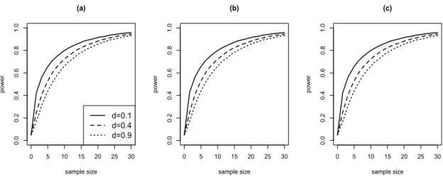
To illustrate the sample size approximation, we consider the models in Simulation 1 withd= 0.1, 0.4 and 0.9. We derive the power ofF-test as a function of sample size under global effect size Gf SN R = 0.2, 0.4 and 0.8, representing small, medium and

large effect size, with type I error at α = 0.05. Here sample size means the number of observations in each group for balanced experiment. The powers from F-test are presented and F∗_{-test gives almost the same result.}

Figure 2.2 displays the power curves from three global effect sizes under three magnitudes of dependency. First of all, it can be seen that the power of F-test achieves 0.8 or more even with moderate sample size, around 20, under medium effect size. Secondly, we can see the effect of within-curve dependency in sample size estimation. Obviously, the covariance structure with strong within-curve correlation needs more sample to achieve the same level of power compared to others. It is corresponding to what we found in Figure 2.1 (a).

(34)

2.4 Real Data Analysis

2.4.1 Analysis of Mouse and Rat Mammary Tumor Data

We now return to the quantitative ultrasound study. The experiment was conducted with two types of mammary tumors, 13 induced 4T1 tumors on mice and 8 induced MAT tumors on rats. The features of tumor tissues, such as length, height and volume vary across subjects. As mentioned in the introduction, the tumor in each animal is invasively scanned by 5 different transducers from three systems (Siemens, Ultrasonix and VisualSonics) which cover different range of frequency bandwidths. Two transducers, 9L4 and 18L6, from Siemens, L14-5 from Ultrasonix, and MS200 from VisualSonics cover frequencies around 3-13.5 MHz, meanwhile MS400 from Vi-sualSonics covers higher frequencies greater than 13.5 MHz. Different from Wirtzfeld et al. (2015), we use the subset of data composed of subjects having large tumor (greater than 70mm3) in the analysis. The data pertain to 5 4T1 and 6 MAT large tumors. Large tumor enables transducer to scan the target without much being affected by surrounding normal tissues, so that noise error has been substantially reduced (Wirtzfeld et al., 2015). From here on, we distinguish 55 combinations of animals and transducers by defining variable called as ‘setup’. For each setup, there are 4 or 5 multiple functional records by shifting scan lines within each tumor. The frequency dependent backscatter (BSC) functions were calculated in decibel scale (dB) for each scan based on the collected ultrasound radio frequency signals using a reference phantom technique. More details can be found in Wirtzfeld et al. (2015).

The aims of this experiment are as follows: Firstly we want to analyze how well BSC records can separate two tumor types by measuring effect size beyond significance test. Secondly, we are interested in finding the frequencies which achieve the most sufficient precision to distinguish two tumors. Lastly, inter-transducer variation in

(35)

BSC is of interest.

Prior to proceeding, note that the repeated measures for each ‘setup’ lead corre-lation structure between multiple curves. The mixed ANOVA result with ‘setup’ as random effect and tumor type as fixed effect is presented in Figure 2.3. They are smoothed from pointwise result via natural cubic splines for comprehensible visual-ization. The smoothed classic 1-way ANOVA result is shown as well for comparison. We see that the magnitude of marginal error in 1-way ANOVA mostly includes both subject and noise random errors.

The collected BSC curves from Ultrasonix L14-5 are summarize in Figure 2.4. The mean values and standard errors at each grid are presented in (a). Both tumors seem to have nearly constant standard deviation over frequencies. The pointwise and smoothed f SN R are illustrated in (b). This indicates that higher frequencies seem more effective in distinguishing tumors than lower frequencies do.

To make a formal inference, now we apply thef SN Ranalysis. As the transducers all have different bandwidths, 3 frequency ranges are selected to carry out subsequent analyses. The lower frequency range (3-8.5 MHz) includes data from Ultrasonix and Siemens transducers, middle frequency (8.5-13.5 MHz) includes two VisualSonics transducers, and the higher frequency range (13.5-21.9 MHz) includes one transducer MS400, from VisualSonics. Table 2.6 displays estimated global measures and boot-strapped p-values over each range. We use 1500 non-parametric bootboot-strapped samples to performf SN Ranalysis hereafter. As discussed in section 2.4, all scans for a given animal and transducer combination were sampled together to preserve correlation between replicates from the same ‘setup’

We see in Table 2.6 that two types of proposed global measures give almost the same significant tumor effect size with small p-value. The estimated measures at each range suggest that higher frequencies are more effective in separating two different

(36)

tu-mors. Figure2.5presents the estimate of smoothedf SN Rusing natural cubic splines with six interior knots selected from BIC, and its 90% pointwise confidence intervals via bootstrapping.(Efron and Tibshirani, 1993). It can yield valuable information about which interval can distinguish two tumors with the most sufficient precision. It demonstrates a trend in increasing separation between MAT and 4T1, which is in agreement with what we found in Table 2.6 and this trend can be explained by the inverse relationship between frequency and wavelength. Higher frequency with short wavelength might collect more information when penetrating a tissue rather than lower frequency with long wavelength can do. Also higher frequencies have relatively wide widths of confidence interval due to small number of curves collected over there. As a next step, we can compare the efficacy of transducers by comparing estimates of effect size. Table 2.7 presents that transducers covering frequencies less than 13.5 MHz have similar significant effect size around 0.8-0.9 with small p-values except Siemens 9L4. The different behavior in Siemens 9L4 seems to be due to influential observations from 4T1 tumor. For relatively higher frequency range, VisualSonics MS400 apparently shows significantly greater separation with larger effect size, which is corresponding to our finding through Table 2.6 and Figure2.5.

The last goal is to examine consistency across systems. For this purpose, we use lower and middle frequency ranges that include at least two transducers, and calculate the global measures to investigate the existence of transducer effect for each tumor type. Specifically, Ultrasonix and Siemens are compared over 3-8.5 MHz and VisaulSonics are compared over 8.5-13.5 MHz. Table 2.8 shows that all estimated measures are less than 0.3 with bootstrapped p-values greater than 0.2, thus the claim of consistency across systems is statistically supported. A key observation is that the magnitudes of transducer effect size are much less than those of tumor effect size.

(37)

2.4.2 Canadian Weather Data

We analyze the Canadian weather data to illustrate the usefulness of our methodology. The data are the daily temperature and precipitation records of 35 weather stations over a year, 365 days, among which 15 in Atlantic, 12 in Continental, 5 in Pacific and 3 in Arctic. The weather information from each station is collected every day with no missing. The dataset is available through R-package ‘fda’. Various functional data analysis methods were already applied by many authors, including statistical inferences to test significant region effect on temperature. Ramsay and Silverman (2005) characterized the typical temperature pattern and investigated when regional temperature effect is substantial by examining F-ratio f unction. However, although pointwise F-ratio can be used to infer an effect size, the sample size or the number of groups should be known in order to be interpreted. Accordingly, it is hard to compare two statistics in general if they are computed from different designs. Also they did not discuss whether the change of regional effect over a year is statistically significant. Zhang and Liang (2007) assessed the significant differences in temperature between climate zones and investigated its pattern over seasons. However, the change in the magnitude of region effect over seasons was just inferred by comparing the magnitude of p-values, not from precise statistical inference. Here our goals are to quantify region effect on temperature and precipitation by applying proposed f SN R analysis, and see when substantial difference between regions is observed. We will also study if the change of effect size over time is significant via bootstrapped confidence intervals of f SN R. Additionally we will see which variable is more affected by geographical factor, among temperature and precipitation.

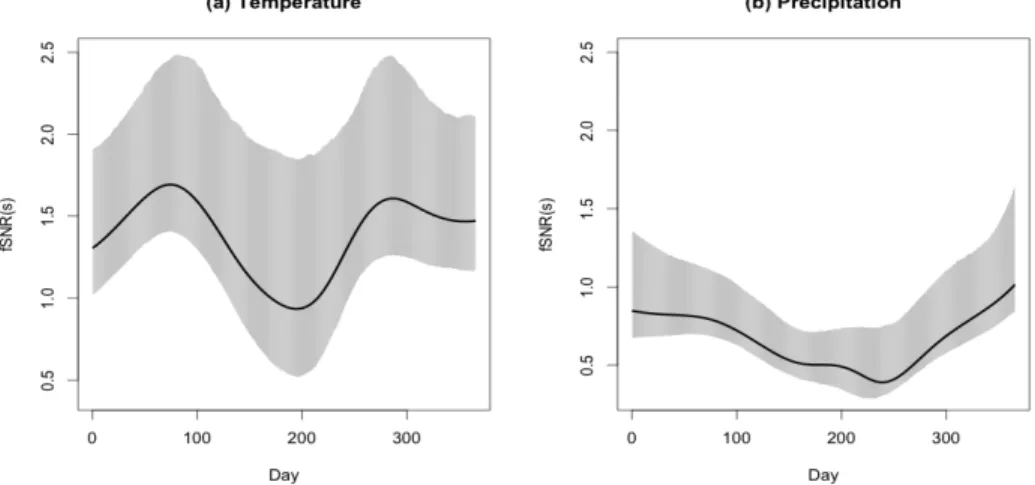
Figure 2.6 presents the estimated f SN R and its bootstrapped 90% confidence intervals over a year based on 1500 bootstrapped samples. Natural cubic splines with

(38)

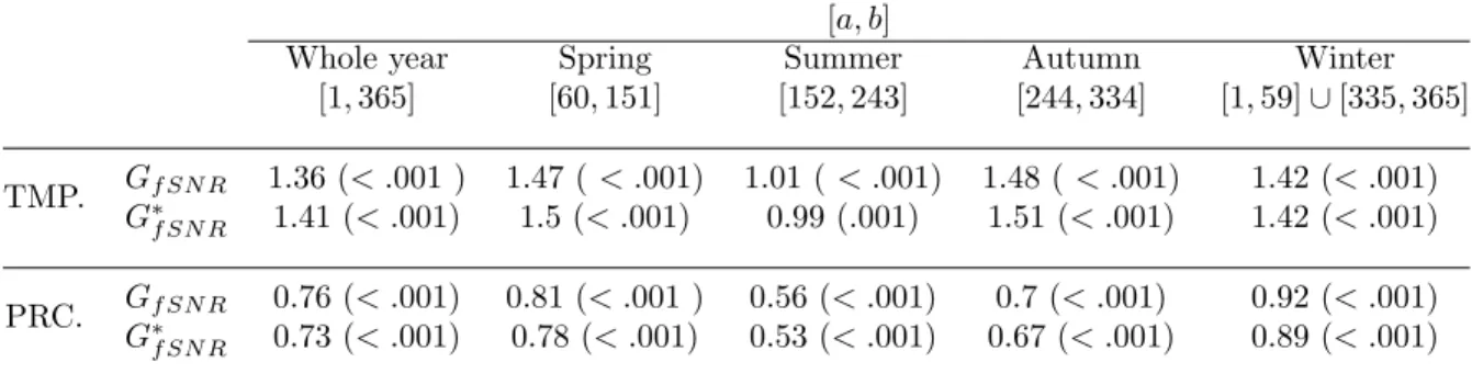
9 interior knot are used to smooth group mean and marginal error curves. It is seen that the difference of temperature between regions is larger than the difference of precipitation with larger estimated effect sizes over the whole year ([a, b] = [1,365]). Although fANOVA or other proposed test result can give the same conclusion of rejection, f SN R enables to present distinct behaviors over time. Specifically, we observe that magnitudes of region effect are different over seasons. In terms of tem-perature, the difference between climate zones is less during the summer (June, July and August or [a, b] = [152,243]) than the difference during the spring (March, April and May or [a, b] = [60,151]) or the autumn (September, October and November or [a, b] = [244,334]), which is in agreement with what Ramsay and Silverman (2005) ob-served from F-ratiof unction. However, we can make further conclusion that seasonal change of region effect in temperature is not statistically significant. The straight horizontal line can be drawn over a year within bootstrapped confidence intervals at around between 1.5 and 2. From (b), it is seen that the region effect on precipitation is large during the winter and early spring. Different from temperature data, we can conclude that this seasonal change is statistically significant.

Table2.6shows the estimated global measures and bootstrappedp-values. Firstly, we can see the consistency of two measures for each time period. Secondly, as ex-pected, estimated regional effect sizes for temperature data are around twice larger than those for precipitation data for the whole year as well as during each season. Lastly, the magnitudes of the regional differences in temperature and precipitation during the summer are less than the magnitudes during the spring and autumn. Again, all associatedp-values are very close to 0, but the proposed measure provides additional information about an effects size and enables to compare to each other.

(39)

2.5 Discussion

The advantages of f SN R analysis are as follows: The effect size of the variable of interest is simply computed through F-ratio f unctionor functional F-statistics. Via visualization of local information and its corresponding confidence intervals, the most informative domain of the function can be found. The asymptotic lower bound of power can be used as an handy tool for sample size estimation in planning purpose.

In future works, we aim to provide asymptotic null distribution of functional F-statistics under irregular sampling framework. To do this, central limit theorem in Hilbert space for i.i.d. stochastic precess with random interval should be demon-strated. Another goal is to extend f SN Ranalysis to 2-dimensional data to quantify the effect size retaining inherent spatial smoothness, to visualize the local effect size in 2-dimensional space and to derive confidence region. It will enable to implement statistical inferences for ultrasound image data for tumor margin assessment as well as spatial data.

(40)

2.6 Figures and Tables

0.0 0.1 0.2 0.3 0.4 0.5 0.6 0.2 0.4 0.6 0.8 1.0 n=20 simulation1 effect size power d=0.1, A d=0.1, S d=0.4, A d=0.4, S d=0.9, A d=0.9, S 0.0 0.1 0.2 0.3 0.4 0.5 0.6 0.2 0.4 0.6 0.8 1.0 n=50 simulation1 effect size power 0.0 0.1 0.2 0.3 0.4 0.5 0.6 0.2 0.4 0.6 0.8 1.0 n=100 simulation1 effect size power 0.0 0.1 0.2 0.3 0.4 0.5 0.6 0.2 0.4 0.6 0.8 1.0 n=20 simulation2 effect size power d=0.4, A d=0.4, S 0.0 0.1 0.2 0.3 0.4 0.5 0.6 0.2 0.4 0.6 0.8 1.0 n=50 simulation2 effect size power 0.0 0.1 0.2 0.3 0.4 0.5 0.6 0.2 0.4 0.6 0.8 1.0 n=100 simulation2 effect size power

(a) Approximated and simulated power curves of F-test on Simulation 1 and 2

0.0 0.1 0.2 0.3 0.4 0.5 0.6 0.2 0.4 0.6 0.8 1.0 n=20 simulation3 effect size power F-test, d=0.4, A F-test, d=0.4, S F*-test, d=0.4, A F*-test, d=0.4, S 0.0 0.1 0.2 0.3 0.4 0.5 0.6 0.2 0.4 0.6 0.8 1.0 n=50 simulation3 effect size power 0.0 0.1 0.2 0.3 0.4 0.5 0.6 0.2 0.4 0.6 0.8 1.0 n=100 simulation3 effect size power

(b) Approximated and simulated power curves of F and F∗-test on Simulation 3 Figure 2.1: Approximated (“A”) and simulated (“S”) power curves as a function of effect size on each scenario.

(41)

0 5 10 15 20 25 30 0.0 0.2 0.4 0.6 0.8 1.0 (a) sample size power d=0.1 d=0.4 d=0.9 0 5 10 15 20 25 30 0.0 0.2 0.4 0.6 0.8 1.0 (b) sample size power 0 5 10 15 20 25 30 0.0 0.2 0.4 0.6 0.8 1.0 (c) sample size power

Figure 2.2: Power functions under d = 0.1, 0.4 and 0.9 for (a) Gf SN R = 0.2, (b)

Gf SN R= 0.4 and (c) Gf SN R= 0.8 5 10 15 20 0 2 4 6 8 Frequency (MHz) tumor effect noise error subject effect 5 10 15 20 0 2 4 6 8 Frequency (MHz) tumor effect marginal error

Figure 2.3: (Top) Pointwise estimate of the difference in magnitude of the BSC esti-mates between two tumors, noise error, and random effect for ‘setup’ from pointwise mixed ANOVA. (Bottom) pointwise tumor effect and marginal error from pointwise 1-way ANOVA

(42)

3 4 5 6 7 8 -4 0 -3 5 -3 0 (a) Frequency (MHz) BSC (d B) 4T1 MAT 3 4 5 6 7 8 0.0 0.5 1.0 (b) Frequency (MHz) fSN R (s) Pointwise fSNR Smoothed fSNR

Figure 2.4: Transducer L14-5. (a) The average and SD curves of 4T1 and MAT, (b) Pointwise and smoothed f SN R

(43)

Figure 2.6: The smoothedf SN R and bootstrapped 90% confidence intervals of (a) Temperature and (b) Precipitation

(44)

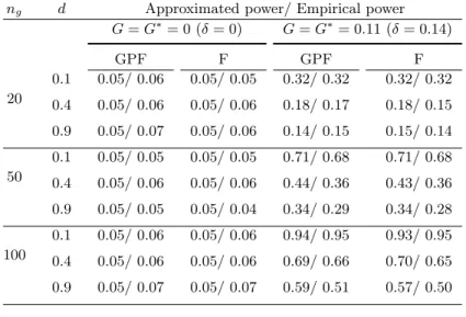
Table 2.1: Simulation 1: approximated and empirical sizes and powers of the F- and F∗_{-test under stationary process model (}_G₌_G

f SN R, G∗ =G∗f SN R)

ng d Approximated power/ Empirical power

G=G∗= 0 (δ= 0) G=G∗= 0.11 (δ= 0.14) GPF F GPF F 20 0.1 0.05/ 0.06 0.05/ 0.05 0.32/ 0.32 0.32/ 0.32 0.4 0.05/ 0.06 0.05/ 0.06 0.18/ 0.17 0.18/ 0.15 0.9 0.05/ 0.07 0.05/ 0.06 0.14/ 0.15 0.15/ 0.14 50 0.1 0.05/ 0.05 0.05/ 0.05 0.71/ 0.68 0.71/ 0.68 0.4 0.05/ 0.06 0.05/ 0.06 0.44/ 0.36 0.43/ 0.36 0.9 0.05/ 0.05 0.05/ 0.04 0.34/ 0.29 0.34/ 0.28 100 0.1 0.05/ 0.06 0.05/ 0.06 0.94/ 0.95 0.93/ 0.95 0.4 0.05/ 0.06 0.05/ 0.06 0.69/ 0.66 0.70/ 0.65 0.9 0.05/ 0.07 0.05/ 0.07 0.59/ 0.51 0.57/ 0.50

ng d Approximated power/ Empirical power

G=G∗= 0.19 (δ= 0.23) G=G∗= 0.26 (δ= 0.32) GPF F GPF F 20 0.1 0.76/ 0.72 0.74/ 0.72 0.95/ 0.97 0.95/ 0.97 0.4 0.47/ 0.44 0.48/0.41 0.73/ 0.68 0.72/ 0.66 0.9 0.37/ 0.34 0.36/ 0.32 0.62/ 0.55 0.62/ 0.52 50 0.1 0.98/ 0.99 0.98/ 0.99 1.00/ 1.00 1.00/ 1.00 0.4 0.81/ 0.81 0.81/ 0.80 0.96/ 0.99 0.96/ 0.98 0.9 0.71/ 0.65 0.70/ 0.64 0.90/ 0.92 0.90/ 0.92 100 0.1 1.00/ 1.00 1.00/ 1.00 1.00/ 1.00 1.00/ 1.00 0.4 0.95/ 0.99 0.96/ 0.98 1.00/ 1.00 1.00/ 1.00 0.9 0.91/ 0.95 0.91/ 0.94 0.99/ 1.00 0.99/ 1.00

(45)

Table 2.2: Simulation 2: approximated and empirical sizes and powers of F- and F∗_{-test under the model with cyclic marginal error function}

ni Approximated power/ Empirical power

G=G∗= 0 (δ= 0) G=G∗=.18 (δ= 13) G=G∗=.28 (δ= 19) G=G∗=.41 (δ= 29)

GPF F GPF F GPF F GPF F

20 0.05/ 0.05 0.05/ 0.05 0.25/ 0.24 0.26/ 0.22 0.54/ 0.48 0.53/ 0.46 0.82/ 0.83 0.83/ 0.81

50 0.05/ 0.04 0.05/ 0.04 0.57/ 0.50 0.59/ 0.49 086/ 0.87 0.86/ 0.87 0.98/ 1.00 0.98/ 1.00

100 0.05/ 0.04 0.05/ 0.04 0.82/ 0.82 0.82/ 0.82 0.97/ 1.00 0.97/ 1.00 1.00/ 1.00 1.00/ 1.00

Table 2.3: Simulation 3: approximated and empirical sizes and powers of F- and F∗_{-test under heteroscedisticity model}

ng Approximated power/ Empirical power

G=G∗= 0 (δ= 0) G=.14, G∗=.11 (δ=.27)

GPF F GPF F

20 0.05/ 0.05 0.05/ 0.05 0.26/ 0.24 0.14/ 0.14

50 0.05/ 0.07 0.05/ 0.06 0.59/ 0.53 0.37/ 0.31

100 0.05/ 0.05 0.05/ 0.05 0.85/ 0.84 0.66/ 0.60

ng Approximated power/ Empirical power

G=.21, G∗=.16 (δ=.41) G=.25, G∗=.20 (δ=.50)

GPF F GPF F

20 0.55/ 0.51 0.34/ 0.28 0.72/ 0.67 0.49/ 0.40

50 0.88/ 0.90 0.69/ 0.64 0.95/ 0.97 0.85/ 0.87

(46)

Table 2.4: Simulation 4: approximated and empirical sizes and powers of F- and F∗_{-test under the model with non-parallel mean functions}

ni Approximated power/ Empirical power

G=G∗= 0 (ϕ= 0) G=G∗=.11 (ϕ=.45) G=G∗=.24 (ϕ= 1) G=G∗=.22 (ϕ=.91)

GPF F GPF F GPF F GPF F

20 0.05/ 0.07 0.05/ 0.06 0.13/ 0.15 0.13/ 0.14 0.38/ 0.38 0.39/ 0.36 0.73/0.74 0.74/ 0.71

50 0.05/ 0.05 0.05/ 0.05 0.38/ 0.36 0.38/ 0.34 0.85/ 0.87 0.86/ 0.86 0.99/ 1.00 0.99/ 0.99

100 0.05/ 0.06 0.05/ 0.06 0.75/ 0.74 0.75/ 0.73 0.99/ 1.00 0.99/ 1.00 1.00/ 1.00 1.00/ 1.00

Table 2.5: Simulation 5: approximated and empirical sizes and powers of F- and F∗_{-test under non-stationary process model}

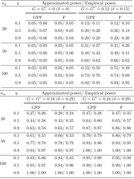
ng η Approximated power/ Empirical power

G=G∗= 0 (δ= 0) G=G∗= 0.12 (δ= 0.15) GPF F GPF F 20 0.1 0.05/ 0.06 0.05/ 0.05 0.13/ 0.11 0.12/ 0.10 0.5 0.05/ 0.07 0.05/ 0.05 0.20/ 0.20 0.20/ 0.18 0.9 0.05/ 0.06 0.05/ 0.04 0.29/ 0.28 0.28/ 0.26 50 0.1 0.05/ 0.05 0.05/ 0.05 0.31/ 0.27 0.31/ 0.26 0.5 0.05/ 0.06 0.05/ 0.06 0.48/ 0.42 0.49/ 0.41 0.9 0.05/ 0.05 0.05/ 0.04 0.68/ 0.62 0.66/ 0.62 100 0.1 0.05/ 0.05 0.05/ 0.05 0.53/ 0.50 0.55/ 0.49 0.5 0.05/ 0.05 0.05/ 0.04 0.73/ 0.70 0.74/ 0.69 0.9 0.05/ 0.05 0.05/ 0.05 0.92/ 0.95 0.93/ 0.95

ng η Approximated power/ Empirical power

G=G∗= 0.18 (δ= 0.22) G=G∗= 0.24 (δ= 0.29) GPF F GPF F 20 0.1 0.27/ 0.26 0.28/ 0.24 0.47/ 0.38 0.47/ 0.35 0.5 0.44/ 0.38 0.43/ 0.35 0.64/ 0.60 0.63/ 0.57 0.9 0.63/ 0.58 0.63/ 0.57 0.87/ 0.87 0.86/ 0.86 50 0.1 0.61/ 0.55 0.60/ 0.53 0.79/ 0.79 0.80/ 0.79 0.5 0.77/ 0.78 0.78/ 0.78 0.93/ 0.96 0.93/ 0.95 0.9 0.94/ 0.97 0.95/ 0.97 1.00/ 1.00 1.00/ 1.00 100 0.1 0.83/ 0.86 0.84/ 0.85 0.95/ 0.98 0.95/ 0.98 0.5 0.95/ 0.97 0.94/ 0.96 0.99/ 1.00 0.99/ 1.00 0.9 1.00/ 1.00 1.00/ 1.00 1.00/ 1.00 1.00/ 1.00

(47)

Table 2.6: Estimates of tumor effect size (bootstrappedp-values in parentheses) Low (3-8.5 MHz) Middle (8.5-13.5 MHz) High (13.5-21.9 MHz) ˆ

Gf SN R 0.56 (< .001) 0.99 (< .001) 1.06 (0.005)

ˆ

G∗_{f SN R} 0.55 (< .001) 0.99 (< .001) 1.06 (0.008)

Table 2.7: Tumor type effect size for each transducer

Transducer _ˆ Gf SN R / ˆG∗f SN R p-value Bandwidth Ultrasonix L14-5 0.78/ 0.73 0.005∗/0.008∗ (3-8.5 MHz) Siemens 9L4 0.17/ 0.13 0.49/0.57 (3-10.8 MHz) Siemens 18L6 0.99/ 0.91 0.004∗/0.007∗ (3-10.8 MHz) VisualSonics MS200 0.87/ 0.84 0.02∗/0.02∗ ( 8.5-13.5 MHz) VisualSonics MS400 1.14/ 1.12 0.004∗/0.004∗ ( 8.5-21.9 MHz)

Table 2.8: Transducer effect size for each tumor type and frequency range Tumor type Frequency range Gˆf SN R / ˆG∗f SN R p-value

4T1 3 -8.5 MHz 0.31/ 0.31 0.34/0.34 8.5 -13.5 MHz 0.27/ 0.26 0.16/0.17 MAT 3 -8.5 MHz 0.28 /0.28 0.25/0.24 8.5-13.5 MHz 0.21/ 0.18 0.44/ 0.50

(48)

Table 2.9: The regional effect size for the Canadian daily temperature and precipi-tation data (with bootstrap p-values in parentheses)

[a, b]

Whole year Spring Summer Autumn Winter

[1,365] [60,151] [152,243] [244,334] [1,59]∪[335,365]

TMP. Gf SN R 1.36 (< .001 ) 1.47 (< .001) 1.01 ( < .001) 1.48 (< .001) 1.42 (< .001)

G∗_{f SN R} 1.41 (< .001) 1.5 (< .001) 0.99 (.001) 1.51 (< .001) 1.42 (< .001)

PRC. Gf SN R 0.76 (< .001) 0.81 (< .001 ) 0.56 (< .001) 0.7 (< .001) 0.92 (< .001) G∗_{f SN R} 0.73 (< .001) 0.78 (< .001) 0.53 (< .001) 0.67 (< .001) 0.89 (< .001)

(49)

2.7 Technical conditions, proof and numerical

algorithm

2.7.1 Condition A

(A.1) µ0(s) andβi(s), i= 1, ..., k ∈L2(S) and tr(γ)<∞.

(A.2) The marginal error processi(s), i= 1, ..., k are i.i.d.

(A.3) As n→ ∞, the k sample sizes satisfyni/N →ai ∈(0,1), i= 1, ..., k.

(A.4) The marginal error process1(s) satisfies Ek1k4 =E[

R

S

2

1(s)ds]2 <∞.

(A.5) For any s ∈ S, γ(s, s) > 0. In addition, the maximum variance m = maxs∈S

γ(s, s)<∞

(A.6) The expectationE[2₁(s)2₁(t)] is uniformly bounded. That is, for any (s, t)∈ S2_,

we haveE[2

1(s)21(t)]< C <∞, whereC is some constant independent of (s, t).

2.7.2 Condition B

(B.1) δ2

r 6= 0 for at least one r ∈ {1, ..., m}

2.7.3 Missing data frame work for irregular functional data

(

2.5 )

Let ¯y(s) = Pn i=1yic(s)1[_Li,Ui](s)/n Pn i=11[_Li,Ui](s)/n 4 = W_W1₂. For each s∈ S, W1 p →E[(y_ic(s)₁[Li,Ui](s)] =E[yci(s)]P(s∈[Li, Ui]),

(50)

by law of large numbers and independence assumption of yc₍_s_{) and} _I_{. Similarly}

W2 p

→P(s ∈[Li, Ui]).

By continuous mapping theorem, W1/W2 p →µ(s). Next, let ˆ σ2(s) = Pn i=1(y c i(s)−y¯(s))21[Li,Ui](s)/n Pn i=11[Li,Ui](s)/n−1/n 4 = W 0 1 W0 2 . For each s∈ S, W₁0 →p E[yc_i(s)−y¯(s)]2P(s∈[Li, Ui]) =E[yc_i(s)−µ(s)]2P(s ∈[Li, Ui]) +E[¯y(s)−µ(s)]2P(s∈[Li, Ui]) =σ2(s)P(s ∈[Li, Ui]) +σ2(s)P(s∈[Li, Ui])/n =σ2(s)P(s ∈[Li, Ui]) +o(1), W₂0 →p P(s∈[Li, Ui])

by continuous mapping theorem, W₁0/W₂0 →p σ2(s)

2.7.4 Power of

F

_s∗

- test

(

2.18 )

We follow the method of proof given in Zhang (2011) and Zhang and Liang (2014) with modification. While Zhang (2011) restricted 0≤τ <1 for further two steps of approx-imation for the local alternative,Hc

1n :Cβ(s)−c(s) = n

−τ /2_d₍_s₎_,_{we simplified proof}

by just using two asymptotic distributions for M SW ∼ AN[tr(γ),2tr(γ⊗2₎_/₍_N ₋

k−1)] and M SB =d Pm r=1λrAr/(k−1) + Pm r=1λ 1/2 r δrzqr/(k−1) +δ2/(k−1), where

Ar ∼χ2k−1. It improves the accuracy of the resulting approximation even for moderate

Effect size estimation and robust classification for irregularly sampled functional data

Abstract

Table of Contents

List of Figures

List of Tables

Chapter 1

Introduction

Chapter 2

Effect Size and Power Analysis for

Functional ANOVA

2.1

Introduction

2.2

Functional Signal-to-Noise Ratio

2.2.1

Missing data framework for irregular functional data

2.2.2

Application to functional ANOVA Model

2.2.3

Pointwise and smoothed estimates of

f SN R

2.2.4

Large sample approximation and bootstrap testing

2.3

Power Analysis

2.3.1

Asymptotic power approximation

2.3.2

Asymptotic versus simulated power on moderate

sample size

2.3.3

Sample size determination

2.4

Real Data Analysis

2.4.1

Analysis of Mouse and Rat Mammary Tumor Data

2.4.2

Canadian Weather Data

2.5

Discussion

2.6

Figures and Tables

2.7

Technical conditions, proof and numerical

algorithm

2.7.1

Condition A

2.7.2

Condition B

2.7.3

Missing data frame work for irregular functional data

(

2.5

)

2.7.4

Power of

F

- test

(

2.18

)