EFFECTS OF CONDITIONING ON THE CONVERGENCE OF RANDOMIZED OPTIMIZATION ALGORITHMS
A Dissertation
Presented to the Faculty of the Graduate School of Cornell University
in Partial Fulfillment of the Requirements for the Degree of Doctor of Philosophy
by
Dennis John Leventhal August 2009
c
2009 Dennis John Leventhal ALL RIGHTS RESERVED
EFFECTS OF CONDITIONING ON THE CONVERGENCE OF RANDOMIZED OPTIMIZATION ALGORITHMS
Dennis John Leventhal, Ph.D. Cornell University 2009
The connection between the conditioning of a problem instance—the sensitivity of a problem instance to perturbations in the input—and the speed of certain it-erative algorithms in solving that problem instance is a recurring topic of study in numerical analysis. This dissertation, consisting of three distinct parts, pro-vides a further connection through the framework of randomized optimization algorithms.
In Part I, we explore how randomization can help asymptotic convergence prop-erties of simple, directional search-based optimization methods. Specifically, we develop a randomized, iterative scheme for estimating the Hessian matrix of a twice-differentiable function. Using this estimation technique, we analyze how it can be used to enhance a random directional search method. From there, we proceed to develop a conjugate-directional search method that incorporates es-timated Hessian information without requiring direct use of gradients.
In Part II, we turn our focus to randomized variants of two classical algorithms: coordinate descent methods for systems of linear equations and iterated pro-jection methods for systems of linear inequalities. We then demonstrate that, under appropriate randomization schemes, linear rates of convergence can be bounded (in expectation) in terms of natural linear-algebraic conditioning
mea-sures for these problems. By considering conditioning concepts induced by met-ric regularity and metmet-ric subregularity, we then expand upon these results by examining randomized projection algorithms for convex feasibility problems. Extensions to reflection-based algorithms are also discussed.
Observing that convex feasibility problems can be reformulated into the prob-lem of finding a common zero of maximal monotone operators, we proceed by studying the proximal point method in Part III. Specifically, for the problem of finding a zero of a single maximal monotone operator, we show that metric subregularity of that operator is sufficient for linear convergence of the proxi-mal point method, leading to a convergence rate in terms of the conditioning induced by the modulus of subregularity. This result is then generalized—by considering randomized and averaged proximal point methods—to obtain a convergence rate for the problem of finding a common zero of finitely many such operators.
BIOGRAPHICAL SKETCH
Originally born in New York City, Dennis spent the first eighteen years of his life in Old Bridge, New Jersey, graduating from Old Bridge High School in June 2000. From there, he moved to Pittsburgh, Pennsylvania to attend Carnegie Mellon University and obtained his B.S. in Mathematical Sciences in Decem-ber 2003 while simultaneously developing minor obsession with the Pittsburgh Steelers. After a six month escape from living in the northeastern United States by moving to the coast of central Florida, Dennis arrived in Ithaca, New York to study Operations Research at Cornell University.
Having recently completed his doctoral studies, Dennis became forced to con-clude that spending 22 years in school makes for a relatively uninteresting bi-ography.
Yeah well, that’s just, ya know, like, your opinion, man. —Jeffrey Lebowski aka The Dude
ACKNOWLEDGEMENTS
First and foremost, I would like to thank my dissertation advisor, Adrian Lewis, without whom this work would not have been possible. His mathematical in-sight has immensely broadened my view of Optimization. Further, his patience and encouragement during the development of this work certainly added to the overall experience.
Next, I would like to thank the other members of my dissertation committee, James Renegar and Michael Todd, not only for the interesting mathematical discussions over the years, but also for providing the initial encouragement to come study Operations Research at Cornell in the first place. Additionally, I’d like to thank Shane Henderson both for his interest in my work and for the help-ful comments and suggestions along the way. More generally, I’d like to extend thanks to Cornell University’s School of Operations Research and Information Engineering and its faculty, students and staff for making this a wonderful place to study.
Additionally, I’d like to thank my parents for their support during this ordeal and, most importantly, listening to me rant on many occasions.
Finally, I’d like to thank the many friends and acquaintances over the years— too many to name individually (though the two of them who may actually read this will undoubtedly take it personally)—for some combination of the support, encouragement or sheer entertainment value they’ve provided, even though I know most of them would vehemently deny having contributed to the “sup-port” or “encouragement” categories.
TABLE OF CONTENTS
Biographical Sketch . . . iii
Dedication . . . iv
Acknowledgements . . . v
Table of Contents . . . vi
List of Figures . . . vii
1 Introduction 1 2 Common Notation and Definitions 11 2.1 Introduction . . . 11
2.2 Linear Algebra . . . 12
2.3 Convex and Variational Analysis . . . 14
2.3.1 The Basics . . . 14
2.3.2 Metric Regularity and Subregularity . . . 17
2.3.3 Geometry and Metric Regularity . . . 21
2.4 Linear Convergence . . . 23
3 Randomized Hessian Estimation 26 3.1 Introduction . . . 26
3.2 Randomized Hessian Estimation . . . 30
3.3 Applications to Algorithms . . . 36
3.3.1 Random Search, Revisited . . . 36
3.3.2 A Conjugate Directions Algorithm . . . 38
3.4 Concluding Remarks for Chapter 3 . . . 48
4 Randomized Methods for Linear Constraints 50 4.1 Introduction . . . 50
4.2 Randomized Coordinate Descent . . . 51
4.2.1 The Basic Result: Positive Semi-Definite Systems . . . 51
4.2.2 The General Result: Positive Semi-Definite Systems . . . . 55
4.2.3 General Linear Systems . . . 57
4.3 Randomized Iterated Projections . . . 59
4.4 Metric Regularity and Local Convergence . . . 68
4.5 Reflection Methods . . . 73
4.5.1 Linear Constraints . . . 75
4.5.2 Convex Constraints . . . 78
4.6 Concluding Remarks . . . 81
5 Randomized Proximal Point Methods 83 5.1 Introduction . . . 83
5.2 Metric Subregularity and Linear Convergence . . . 86
5.2.1 The Main Results . . . 86
6 Open Questions and Future Research 96
LIST OF FIGURES
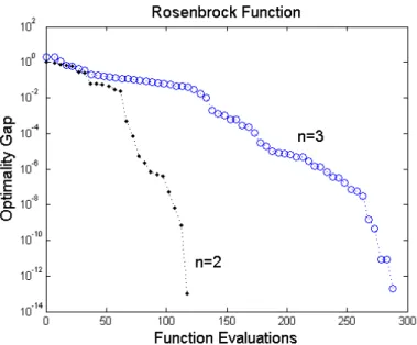
3.1 Random search with Hessian estimates on convex quadratics . . 39 3.2 Conjugate directions algorithm on convex quadratics . . . 46 3.3 Conjugate directions algorithm on Rosenbrock function . . . 47 3.4 Conjugate directions and Nelder-Mead algorithms . . . 48 4.1 Randomized coordinate descent algorithm for least squares
problems . . . 60 4.2 Randomized alternating projection algorithm for linear
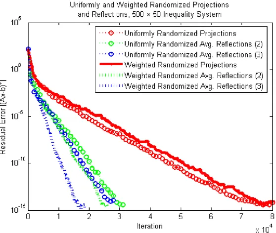
inequal-ities . . . 66 4.3 Randomized Reflections of Equality Systems . . . 78 4.4 Randomized Reflections for Inequality Systems . . . 79
CHAPTER 1 INTRODUCTION
The condition number of a problem instance measures the sensitivity of a solu-tion to small perturbasolu-tions in its input data. For many problems that arise in numerical analysis, there is often a simple relationship between the condition number of a problem instance and the distance to the set ofill-posed problems— those problem instances whose condition numbers are infinite [28]. For exam-ple, with respect to the problem of inverting a matrixA, it is known (see [59], for example) that ifAis perturbed toA+E for sufficiently smallE, then
k(A+E)−1−A−1k
kA−1k ≤ kA
−1k kEk+O(kEk2).
Thus, a condition measure for this problem may be taken askA−1k. Associated with this is the classical Eckart-Young theorem found in [37], relating the above condition measure to the distance to ill-posedness.
Theorem 1.0.1 (Eckart-Young) For any non-singular matrix,A,
min
G {kGk: A+Gis singular} = 1 kA−1k.
From a computational perspective, a related and important area of study is that of error bounds. Given a subset of a Hilbert space, an error bound is an inequal-ity that bounds the distance from a test vector to the specified subset in terms of some residual function that is typically easy to compute. In that sense, an error bound can be used both as part of a stopping rule during implementation of an algorithm as well as an aide in proving algorithmic convergence. A comprehen-sive survey of error bounds for a variety of problems arising in optimization can be found in [87].
With regards to the problem of solving a square, nonsingular linear system Ax = b, one connection between condition measures and error bounds is im-mediate. Let x∗
be a solution to the system and xbe any other vector. Then kx−x∗k =kA−1A(x−x∗)k=kA−1(Ax−b)k ≤ kA−1k kAx−bk, (1.0.2) so the distance to the solution set is bounded by a constant multiple of the resid-ual vector, kAx−bk, and this constant is the inverse of the one that appears in the context of distance to singularity. Practically speaking, knowledge of the error bound—or of the existence of such an error bound—allows one to know that the distance to the solution set is bounded by a multiple of a more easily-computable quantity—in this case, the residual norm.
The frequent appearance of the termkA−1kin the above results is no coincidence.
A recurring paradigm in the area of numerical analysis is the near-equivalence between badly posed problems—those problems which are a small perturba-tion from being ill-posed—and problems for which weak error bounds exist. Further, these two properties are themselves often associated with problems for which iterative algorithms tend to converge slowly. For example, consider the problem of solving a linear system, Ax = b, where now Ais a positive-definite matrix. Theorem 1.0.1 and Inequality 1.0.2 show that whenkA−1k is large, the
distance to ill-posedness is small and the natural error bound is weak. Further, the steepest descent algorithm and the conjugate gradient algorithm are known to be linearly convergent (see [1], [48], among others) with rates1−O(k(1A))and 1−O(√1
k(A)), respectively, where k(A) = kAk kA
−1k is a scale-invariant condition
measure. If we consider the set of problem instances with a fixed value ofkAk (by considering ana priorirescaling, for example), this shows that these partic-ular iterative algorithms converge more slowly askA−1kincreases.
There is no shortage of literature on the interplay between the ideas of condi-tioning and error bounds and, of particular interest to the optimization commu-nity, algorithmic efficiency. For example, in the pioneering papers by Renegar in [96], [97], [98], a conditioning notion for linear programming was defined di-rectly in an “Eckart-Young style”—in terms of the distance to infeasibility—and it was shown that this condition measure directly governs the speed of interior point algorithms.
Much work exists in other areas of optimization, as well, relating condition-ing, error bounds and algorithmic speed. Sample work includes quadratic pro-gramming [116], nonlinear propro-gramming [112], semidefinite propro-gramming [82], stochastic programming [104] and additional examples for linear programming [110], [57], while a broad variety of applications are discussed in [87] and the many references therein. This list is by no means comprehensive, either across areas of study or within the specifically listed areas.
A broad framework is being built in variational analysis for generalizing this paradigm to nonlinear systems. In the spirit of keeping things as sufficiently general as possible, consider a set-valued mapping, Φ : E →→ Y, satisfying Φ(x)⊆Yforx∈E. An associated problem is that of finding xsuch thatb¯ ∈Φ(x) for a given vectorb. This framework encompasses a variety of problems, includ-¯ ing not only ordinary equation solving, but also feasibility problems, variational inequalities and other optimality conditions.
Naturally, any result will ultimately depend on properties of the mapping Φ itself; however, this general framework of set-valued mappings allows for the exploration of the “true nature” of conditioning without being encumbered by a specific problem structure. Our interest in regularity properties ofΦwill focus
around the area of metric regularity, essentially defined by the existence of a local error bound around( ¯x,b)¯ withb¯ ∈Φ( ¯x). This and related properties will be defined more formally in Section 2.3.2. Thorough surveys about error bounds, metric regularity and related properties can be found in [73], [61] and [33]. Metric regularity provides a broad generalization to the conditioning ideas dis-cussed in the context of linear systems. For example, it’s certainly curious that the constant appearing in the Eckart-Young Theorem, Theorem 1.0.1, is the re-ciprocal of the constant in the natural error bound for linear systems, Inequality 1.0.2. In fact, this inverse relationship between error bounds and distance to ill-posedness is substantially more general. As shown in [32] and discussed briefly in Section 2.3.2, under mild assumptions, metric regularity is the condition un-der which this relationship holds, but for set-valued mappings instead of being limited to linear systems.
Although the nature of metric regularity makes it an interesting topic of study in its own right, further interest in this property is propagated by the implications of metric regularity when studying specific classes of problems or mappings, often leading back to well-studied regularity assumptions for specific problems. Consider a few prominent examples. Given a convex function, f, it was shown in [5] that metric regularity of the subdifferential mapping,∂f, is equivalent to a type of local quadratic growth condition. For a differentiable, convex inequality system
gi(x)≤0 fori=1, . . . ,m, (1.0.3) it was shown in [72] that, under appropriate conditions, metric regularity of the mappingΦ(x) = [g1(x), . . . ,gm(x)]T +Rm+ is equivalent to Abadie’s constraint
([99]) and Mangasarian-Fromowitz ([27]) constraint qualifications. When the constraints in 1.0.3 are restricted to be affine, metric regularity provides a con-nection between the classic Hoffman error bound from [58] and the distance to infeasibility studied by Renegar in [96], among others. Further, as shown in [32, Thm. 4.8], the framework of metric regularity provides an alternative method for calculating the distance to infeasibility in such a case by appealing to con-nections with the calculus of coderivatives (see [103], among others).
Given this connection between error bounds and distance to ill-posedness for set-valued mappings, the question remains as to how this property affects the speed of iterative algorithms. The general use of error bounds to understand the convergence of algorithms has been studied by many authors for a vari-ety of applications; one broad approach that encompasses gradient projection methods, coordinate descent methods and proximal point algorithms, among others, can be found in [77] and [75]. The body of work explicitly establishing a connection between metric regularity and algorithmic performance is still in its infancy; however, the papers [4], [70] and [66] are worthy of mention. This, in fact, is the second of the two major themes we address in this dissertation. Fundamentally, the primary theme of this dissertation involves the introduc-tion of randomizaintroduc-tion schemes in an algorithmic context, though the reasons for doing so vary. The most prominent reason in this dissertation for studying randomized algorithms is to broaden the understanding of the connection be-tween conditioning of a problem instance and the performance of iterative algo-rithms on that problem instance. For example, return to the problem of solving a positive-definite linear system,Ax= b, equivalently formulated as the optimiza-tion problem of minimizing the convex quadratic funcoptimiza-tion f(x) = 12xTAx−bTx
As previously mentioned, the well-studied steepest descent method and con-jugate gradient method are both linearly convergent with rates expressible in terms of the relative condition number,kAk kA−1k.
For many other iterative algorithms for solving this problem, there is a natural “choice” of search directions to be made at each iteration. From the context of solving the optimization problem, for example, the classical coordinate descent method repeatedly cycles through the set of coordinate directions, {e1, . . . ,en},
performing an exact minimization over one variable at each iteration. Alterna-tively, taking the view of solving the underlying linear system, an alternating projections algorithm cycles through the set of equations and obtain the new iterate by orthogonally projecting the current iterate onto the hyperplane asso-ciated with one of the linear equations. These algorithms are of interest because of their low computational cost, each requiring onlyO(n)arithmetic operations per iteration. Further, each of these algorithms is known to be linearly conver-gent, but the rates of convergence are not easily expressible in terms of typical matrix quantities like the condition number. By choosing an appropriate prob-ability distribution over the choice of search directions, however, we can show that the randomized variants of the algorithms satisfy a probabilistic version of linear convergence but with a rate now expressible in terms of classical condi-tioning concepts.
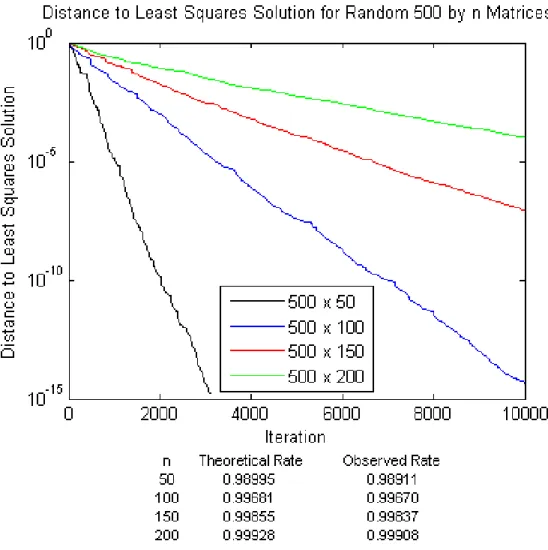
Naturally, we would like generalizations of the above convergence theory to larger classes of problems. A starting point for such a generalization is to con-sider arbitrary linear systemsAx= b, for which we later show that a randomized coordinate descent algorithm is still linearly convergent with a rate dependent on the condition number of A. A recent result of Strohmer and Vershynin in
[109], slightly extended in Corollary 4.3.9, shows a similar convergence result for a randomized projections algorithm which, interestingly enough, has the same convergence rate as the randomized coordinate descent method. Though this connection may seem surprising, it follows naturally from the fact that the analysis of each algorithm relies on the same error bound for the problem in-stance.
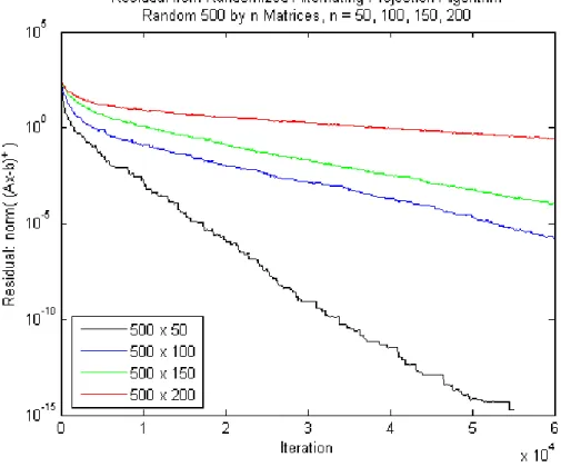
In fact, iterated projection algorithms have been well-studied for broad classes of problems. Using a similar randomization scheme as for linear equations, we proceed to demonstrate linear convergence for a randomized projection algo-rithm for linear inequality systems, Ax ≤ b, with a rate expressible in terms of a natural error bound provided by Hoffman in [58]. Further connecting error bounds and distances to ill-posedness, we also provide a distinct convergence rate in terms of the distance of infeasibility to [96]—originally investigated by Renegar and shown to govern the convergence rate of interior point methods— for a specific implementation of this algorithm.
Building upon these results, we continue by considering randomized projection algorithms for convex feasibility problems. After showing that finding a point in the intersection of closed and convex sets can be reformulated into the prob-lem of finding a zero of a specific set-valued mapping, we proceed by using the error bound provided by metric regularity (or metric subregularity) to demon-strate linear convergence for several types of projection-based algorithms. Observing that the projection operator is actually a special case of the proximal point method leads us in the direction of an even broader problem—finding a zero, or a common zero, of one or more maximal monotone mappings. With regards to the problem of finding a zero of a single mapping, we show that
when the mapping is in fact metrically subregular, the error bound provided by subregularity directly governs the convergence rate of the proximal point algorithm. Even further, similar behavior is shown for the problem of finding a common zero of finitely many maximal monotone operators, via a random-ized proximal point algorithm, and a convergence rate is shown that depends both on the error bound derived from the metric subregularity of the mappings themselves as well as from the metric subregularity of the mapping associated with the solution set, similar in nature to what we observe from the randomized projection algorithm for convex feasibility problems. In fact, as a special case of this, we re-obtain the results on randomized projection algorithms.
Although using randomization techniques to demonstrate a broader connection between error bounds, distance to ill-posedness and algorithmic performance is a recurring theme in this dissertation, it’s certainly not the only reason for con-sidering randomized algorithms. One practical reason is the hope that certain randomization schemes, even unnatural ones, will lead to improved numerical performance when compared with “traditional” algorithms. In fact, in Chap-ter 4, we provide examples where seemingly unnatural randomization schemes demonstrate the potential for improved performance on certain classes of prob-lems when compared with either the traditional, deterministic algorithm or the “natural” randomization scheme.
Although Chapters 4 and 5 primarily revolve around the use of randomiza-tion to understand how condirandomiza-tioning behavior governs the convergence rate of simple algorithms, the main part of this dissertation begins with an alternate approach. In Chapter 3, we examine a method for estimating the conditioning of a twice-differentiable function in terms of the underlying Hessian matrix. In
particular, through an appropriate randomization scheme, we demonstrate an estimation technique that is linearly convergent (in expectation) to the true Hes-sian matrix but, unlike many traditional Newton-like methods, does not require direct gradient information. As an application of this technique, we show how a random search algorithm can be accelerated to provide an asymptotic conver-gence rate independent of the problem’s conditioning. Further, we demonstrate how coordinate descent-style algorithms can be improved to take advantage of the function’s underlying conditioning, leading to superlinear convergence. The “derivative-free” nature of this analysis provides a way of comparing these randomized algorithms with traditional, gradient-based algorithms like steep-est descent and Newton-like methods.
Our initial interest in randomized algorithms stems from the seemingly un-related papers [39] and [42]. In the former paper, certain randomized search schemes are presented as having characteristics of approximation via smooth-ing, even for discontinuous or non-differentiable problems, while connections with more traditional methods of convex analysis are provided. In the latter paper, a random search technique is used to provide provable error results for differentiable, online minimization problems by using the fact that, in expecta-tion, a certain derivative-free randomization scheme has gradient-like proper-ties. In a sense, the ideas of the latter paper provided the motivation for the results in Chapter 3 while the philosophy behind the former paper—as well as recent work in [109]—encouraged the ideas behind Chapters 4 and 5.
In order to develop the ideas discussed in this introduction more fully, this dissertation is organized as follows. Chapter 2 consists of the common nota-tion, definitions and background material that will be frequently referenced in
the remaining chapters. In Chapter 3, we introduce randomized algorithms for solving twice-differentiable optimization problems and compare the results with traditional methods on a cost-per-function-evaluation basis. In Chap-ter 4, we consider randomized algorithms for specific classes of problems— positive-definite linear systems, linear equality and inequality systems, and convex feasibility problems—and show how randomization allows the deter-mination of convergence rates in terms of traditional conditioning measures. In Chapter 5, we further examine the interplay between randomization and metric (sub)regularity, developing new convergence theory for proximal point meth-ods.
In conclusion, we would like to say that Chapter 3 is based on a joint paper with A.S. Lewis accepted for publication in the journalOptimizationat the time of the writing of this dissertation. Chapter 4 is based on a paper with A.S. Lewis submitted for publication toMathematics of Operations Research. Finally, Chapter 5 is based on a paper that has passed through an initial review for theJournal of Mathematical Analysis and Applicationsand is undergoing minor revisions.
CHAPTER 2
COMMON NOTATION AND DEFINITIONS
2.1
Introduction
In this chapter, common notation used throughout this dissertation will be de-fined along with a collection of background results from a variety of mathe-matical areas. For further reading on some recurring topics, sample references include linear algebra ([59], [60]), convex and variational analysis ([25], [103], [55], [18]), approximation theory ([30]) and probability ([17]).
Throughout this dissertation, unless otherwise stated, assume thatEis a Hilbert
space with an inner product h , i and induced norm k · k = h·,·i12. As
fre-quently used examples of Hilbert spaces, denote the spaces of real numbers, n-dimensional real vectors and real-valued symmetric n×nmatrices by R, Rn,
andSnrespectively, each with their usual Euclidean inner products. Also
refer-enced will be the set of non-negative real numbers, R+, and the extended real
numbers, R¯, defined as R∪ {±∞}. When necessary, let Y be a second Hilbert
space whose inner product and norm are denoted identically as above. When-ever possible, we will denote vectors by lowercase letters, constants by lower-case Greek letters, matrices, sets and operators by upperlower-case letters, random variables by bold text and spaces by “blackboard bold,” likeE. In the context of
randomized algorithms, however, the notation for the underlying probabilistic nature of the iterates will be suppressed for simplicity.
On the Hilbert spaceE, denote the closed unit ball byB = {x ∈E : kxk ≤ 1}and
Given two setsUandV andα∈R, define the set operations element-wise by U+V ={u+v:u∈U,v∈V}
and
αU ={αu:u∈U}.
2.2
Linear Algebra
In what follows, consider m-by-n real matrices A. The set of rows of A is de-noted by {aT
1, . . . ,a
T
m}and the set of columns is denoted {A1, . . . ,An}. The
spec-tral norm ofA is the quantity kAk2 := maxkxk=1kAxkand the Frobenius normis
kAkF :=
q P
i,ja2i j. Additionally, these norms satisfy kAk2 ≤ kAkF ≤
√
nkAk2. (2.2.1)
For an arbitrary matrix, A, let kA−1k2 be the smallest constant M such that kAxk2 ≥ 1
Mkxk2 for all vectors x. In the case m ≥ n, if A has singular values σ1 ≥ σ2 ≥ · · · ≥ σn, then M can also be expressed as the reciprocal of the
mini-mum singular valueσn, and, if Ais invertible, this quantity equals the spectral norm ofA−1. Additionally, denote the smallest non-zero singular value of Aby
σ(A).
Now suppose the matrixAisn-by-nand positive definite, being symmetric and satisfyingxTAx>0for allx,0. Theenergy norm(orA-norm), denotedk · kA, is defined bykxkA :=
√
xTAx. This norm satisfies
kAxk2 ≤λmax(A)kxkA2 ≤ λmax(A)2kxk22 (2.2.3) and
λmin(A)kxk22 ≤ kxk 2
A, (2.2.4)
where λmax(A) and λmin(A) are the maximum and minimum eigenvalues of A,
respectively. Further, if A is simply positive semi-definite, we can generalize Inequality 2.2.2:
xTAx≤ 1
λ(A)kAxk2 (2.2.5)
whereλ(A)is the smallest non-zero eigenvalue ofA. We denote the trace ofAby trA: it satisfies the inequality
kAkF ≥ trA
√
n. (2.2.6)
For the frequently associated, strictly convex quadratic function f(x)= 12xTAx+bTxwith minimizer x∗ =−A−1b, the energy norm satisfies
1 2kx− x ∗k2 A = f(x)− f(x ∗). (2.2.7) Observe that Equation2.2.7holds for any solutionx∗toAx=bin the case where Ais only positive semi-definite as long as a solution exists, noting that any such solution is a minimizer of f. However, the left-hand side, defined exactly as before, is no longer technically a norm.
InRn, letei denote the column vector with a 1 in theithposition and zeros
else-where. Additionally, for a vectorx∈Rn, define the vectorx+by(x+)i =max{xi,0} and the matrixDiag (x)to be the matrix whose main diagonal is the vector xand whose other entries are 0.
Certain conditioning measures for linear systems will be frequently referenced. Therelative condition number of Aisk(A) := kAk2 kA−1k2, the commonly used
condition measure. Another measure of interest is the scaled condition num-ber, introduced by Demmel in [29], given byκ(A) := kAkFkA−1k2. In particular,
these measures are related by
k(A)≤ κ(A)≤ √n k(A).
2.3
Convex and Variational Analysis
2.3.1
The Basics
Let F be aset-valued mapping, denoted F : E →→ Y, such that F(x) ⊆ Y for all
x ∈ E. The inverse mapping, denoted F−1, is defined by x ∈ F−1(y) ⇔ y ∈ F(x).
Thegraph, domainand rangeof F, denoted gph F, dom F and rng F are de-fined by
gphF = {(x,y) :y∈F(x)}, domF = {x:F(x),∅} and
rng F =∪x∈EF(x).
A set-valued mapping F is called single-valued on a set, D ⊂ E, denoted F : D → Y, if F(x) is a singleton for all x ∈ D. In such a case, denote F(x) to be either the single-element set or the unique element of that singleton set as appropriate from the context.
Given a set S ⊆ E, the distance from x to S, denoted d(x,S), is defined by inf{kx−zk:z∈S}. IfS is closed and convex, definePS(x)to be theprojection op-eratoronS: that is,PS(x)is the unique vector inS satisfyingkx−PS(x)k=d(x,S).
Definition 2.3.1 A single-valued mappingT :E→ Yisfirmly non-expansiveif
kT(x)−T(y)k2+k(I−T)(x)−(I−T)(y)k2≤ kx−yk2 ∀x,y∈E (2.3.2) andnon-expansiveif
kT(x)−T(y)k ≤ kx−yk ∀x,y∈E, (2.3.3) whereI is the identity mapping.
Proposition 2.3.4 [47, Thm. 12.1] A mappingT is firmly non-expansive if and only if2T −I is non-expansive.
Proposition 2.3.5 The composition of finitely many expansive mappings is a non-expansive mapping.
Proof LetT andU be two non-expansive mappings. Then kT(U(x))−T(U(y))k ≤ kU(x)−U(y)k ≤ kx−yk.
The result then follows by induction. 2
Proposition 2.3.6 [30, Thm. 5.5] For a closed, convex set,S, the projection operator PS(·)is firmly non-expansive.
By observing that PS(x) = xfor all x ∈S, the following inequality derived from Inequality 2.3.2 will prove useful later:
ky−xk2− kPS(y)−xk2 ≥ ky−PS(y)k2 for allx∈S, y∈E. (2.3.7)
Definition 2.3.8 The normal cone to a closed, convex set S at x is defined as NS(x)=∅if x<S and, ifx∈S,
NS(x) :={y∈E: hy,s−xi ≤0 ∀s∈S}. (2.3.9)
The projection operator can be characterized in terms of the normal cone.
Proposition 2.3.10 [30, Thm. 4.1] For a closed convex set,S, the corresponding pro-jection operator can be characterized by
z=PS(x) if and only if z∈S andx−z∈NS(z). (2.3.11)
Specifically,x−PS(x)∈N(PS(x))for all x.
Definition 2.3.12 Given a single-valued function f : E → R¯, the epigraph of f is
defined to be
epif = {(x,y)∈E×R:y≥ f(x)}.
Definition 2.3.13 A single-valued function f : E → R¯ isconvexif its epigraph is a
convex set.
Additionally, for a single-valued function f, the domain of f :E→ R¯ is defined to be the domain of the mapping whose graph is the epigraph of f.
Definition 2.3.14 Thesubdifferentialof a convex function f at x, denoted¯ ∂f( ¯x), is defined by
∂f( ¯x)={y∈E: f(x)≥ f( ¯x)+hy,x− x¯i for all x∈E} forx¯∈domf and∂f( ¯x)=∅otherwise.
Example 2.3.15 Let ιS be the indicator function for S ⊆ E, where S is a closed and convex set, satisfying ιS(x) = 0 when x ∈ S and ιS(x) = ∞ otherwise. Then ∂ιS( ¯x)=NS( ¯x).
LetXbe a random vector onEand letE[·]be the expected value operator with
respect to the probability distribution ofX. The following proposition, known as Jensen’s Inequality, will be frequently used.
Proposition 2.3.16 (Jensen’s Inequality) Let X be a random vector on E and let
f :E→R¯ be a convex function. Then
f(E[X])≤E[f(X)].
2.3.2
Metric Regularity and Subregularity
Consider a set-valued mapping Φ : E →→ Y and the problem of solving the
associated constraint systemb¯ ∈Φ(x)for the unknown vector x. Building upon the idea of an error bound for linear systems as discussed in Chapter 1, we consider related regularity conditions for set-valued mappings. The first is that of metric regularity.
Definition 2.3.17 The set-valued mappingΦ: E→→Yismetrically regularatx¯for
¯
bifb¯ ∈Φ( ¯x)and there existsγ >0such that d(x,Φ−1
(b))≤ γd(b,Φ(x)) for all(x,b)near( ¯x,b).¯ (2.3.18) Themodulus of regularity, denotedRegΦ( ¯x|b), is the infimum of all constants¯ γsuch that Inequality 2.3.18 holds.
Metric regularity generalizes the error bounds previously discussed at the ex-pense of only guaranteeing a bound in local terms. For example, ifΦis a single-valued linear map, then the modulus of regularity (at any x¯ for any b¯) corre-sponds to the typical conditioning measure kΦ−1k
2 (with kΦ−1k2 = ∞ implying
the map is not metrically regular) and ifΦis a smooth single-valued mapping, then the modulus of regularity is the reciprocal of the minimum singular value of the Jacobian,∇Φ(x).
The property of metric regularity possesses strong connections with other ideas in variational analysis. The simplest is that it provides a generalization of the Banach open mapping principle which effectively says, as shown in [32, Ex. 1.1], that a bounded and linear mapping is metrically regular if and only if it is surjec-tive, in which case the modulus of regularity is simplysup{d(0,A−1(y)) : y ∈ B}.
If the mapping Φ has a closed-convex graph, the Robinson-Ursescu Theorem ([111], [100], et. al.) says thatΦis metrically regular at x¯forb¯ if and only ifb¯ is in the interior of the range ofΦ. Metric regularity is additionally known to be equivalent to several other properties in variational analysis, namely the Aubin property ofΦ−1 and the openness at linear rate ofΦ([103, Thm 9.43]). Further,
a result originating with Lyusternik and Graves ([79], [49]) and extended by others (for example, [31],[61], [32]) shows that metric regularity is determined by the first-order behavior of a mapping and is preserved under perturbations of mappings with sufficiently small Lipschitz constant. Additional information about metric regularity and its relationship to other concepts in variational anal-ysis can be found in the surveys [33], [61], among others.
From an alternative perspective, metric regularity provides a framework for generalizing the Eckart-Young result on the distance to ill-posedness of linear
mappings cited in Theorem 1.0.1.
Definition 2.3.19 For a set-valued mappingΦ:E→→Ywith closed graph, theradius
of metric regularityat x¯forb¯ is given by
radΦ( ¯x|b)¯ = inf{kGk:Φ +Gnot metrically regular atx¯forb¯+G( ¯x)}, where the infimum is over all linear mappingsG.
The following strikingly simple relationship between the radius of regularity and the modulus of regularity was shown in [32].
Proposition 2.3.20
radΦ( ¯x|b)¯ ≥ 1 RegΦ( ¯x|b)¯ ,
with equality holding whenΦis a mapping between finite dimensional spaces.
A slightly weaker condition than metric regularity is that of metric subregular-ity, defined as in [62].
Definition 2.3.21 The set-valued mappingΦ :E→→Yismetrically subregularatx¯
forb¯ ∈Φ( ¯x)if there existsγ >0such that d(x,Φ−1
(¯b))≤ γd(¯b,Φ(x))for all xnearx.¯ (2.3.22) Themodulus of subregularity, denotedSubregΦ( ¯x|b), is the infimum of all constants¯ γsuch that Inequality 2.3.22 holds.
Observe that the reference vectorb¯is fixed in Inequality 2.3.22 for metric subreg-ularity, but not in Inequality 2.3.18 for metric regularity; from this, it naturally follows that SubregΦ( ¯x|b)¯ ≤RegΦ( ¯x|b)¯ . In [33], the following, slightly modified definition of metric subregularity is used instead.
Definition 2.3.23 ([33]) The set-valued mappingΦ :E→→Yismetrically
subregu-larat x¯forb¯ ∈Φ( ¯x)if there existsγ >0and a neighborhoodVofb¯ such that d(x,Φ−1(¯b))≤ γd(¯b,Φ(x)∩V)
for all xnearx.¯ (2.3.24)
As noted without proof in [62], the definitions are equivalent in the sense that, given x¯ and b¯ ∈ Φ( ¯x), Definition 2.3.21 holds if and only if Definition 2.3.23 holds. We include a short proof of this equivalence here for completeness.
Proposition 2.3.25 The set-valued mappingΦ : E→→ Yis metrically subregular atx¯
forb¯ according to Definition 2.3.21 if and only if it is metrically subregular at x¯ forb¯ according to Definition 2.3.23.
Proof ⇒: Suppose there existsγ > 0 such that Definition 2.3.21 holds. Then, choosingV =Y, the result follows trivially.
⇐: Let x be sufficiently near x¯ so that Definition 2.3.23 holds with constant γ >0and note that, ifΦ(x)= ∅, then Inequality 2.3.22 holds trivially. Therefore, assumeΦ(x) , ∅. To temporarily abuse some previous notation, define PΦ(x)(¯b)
to be any element of E that attains the infimum of inf{ky− bk¯ : y ∈ cl(Φ(x))},
where cl(S) is the closure of S, implying that d(¯b,Φ(x)) = kb¯ − PΦ(x)(¯b)k. From
this, it follows that
d(x,Φ−1(¯b)) ≤ γd(¯b,Φ(x)∩V) (Inequality 2.3.24) ≤ γhkb¯−PΦ(x)(¯b)k+d(PΦ(x)(¯b),V) i (Triangle Inequality) ≤ 2γkb¯−PΦ(x)(¯b)k (sinceb¯ ∈V) = 2γd(¯b,Φ(x)) (Definition of Projection). 2
Metric subregularity of Φ is shown to be related to the calmness of Φ−1 and
this relationship is thoroughly explored in several papers, including [62] and [115]. Unfortunately, metric subregularity fails to imply many of the stability properties implied by metric regularity. Examples are shown in [33] where met-ric subregularity is not preserved under a perturbation with Lipschitz constant 0, unlike metric regularity. Further, examples are given that show that metric subregularity implies no “natural” relationship between the modulus and the radius of subregularity like the one of Proposition 2.3.20.
2.3.3
Geometry and Metric Regularity
Given closed and convex setsS1, . . . ,Sm ⊆E, we often want to consider regular-ity aspects of the sets themselves. We will examine one approach that involves considering regularity properties of a related set-valued mapping. Endow the product spaceEmwith the inner product
h(u1,u2, . . . ,um),(v1,v2, . . . ,vm)i=
m
X
i=1
hui,vii
and consider the set-valued mappingΦ:E→→Emgiven by
Φ(x)=[S1−x,S2−x, . . . ,Sm− x]T. (2.3.26) Then it clearly follows that x¯ ∈ ∩iSi if and only if0 ∈ Φ( ¯x). Using metric regu-larity as a starting point, supposeΦ(x)is metrically regular at x¯ for 0. From the definition, this is equivalent to thestrong metric inequality, examined in [67] and [68], among others, defined by the existence ofβ, δ > 0such that, fori= 1, . . . ,m,
d(x,∩i(Si−zi))≤βmax
1≤i≤md(x+zi,Si) for allx
Characterizing this in terms of normal cones, it was shown in [68, Thm. 1, Prop. 10, Cor. 2] that this is equivalent to the existence of constantsδ,k >0such that
zi ∈δB, yi ∈NSi( ¯x+zi) (i=1, . . . ,m)⇒ X i
kyik2≤ k2kX i
yik2. (2.3.28) By using the formula in [103, Thm 9.43] for expressing the modulus of regularity in terms of coderivatives, it was shown in [70] that
RegΦ( ¯x|0)=lim
δ↓0
n
inf{k: Inequality 2.3.28 holds.}o. (2.3.29)
As a corollary to Equation 2.3.29, we obtain the following result, which will be useful later, that nicely rephrases Equation 2.3.28.
Corollary 2.3.30 ([70]) Suppose the set-valued mappingΦ(x)=[S1−x, . . . ,Sm−x]T is metrically regular atx¯for 0 and letγ¯ be any constant greater thanRegΦ( ¯x|0). Then for all xi ∈Sisufficiently near x, any vectors¯ yi ∈NSi(xi), i= 1, . . . ,msatisfy
X
i
kyik2≤ γ¯2kX i
yik2.
Consider a relaxed variant of the strong metric inequality, known simply as the metric inequalityas studied in [61], [86] and [68] among others, defined to hold atx¯if there existsβ >0such that
d(x,∩iSi)≤βmax
1≤i≤md(x,Si) for allx∈x¯+δB. (2.3.31) If Inequality 2.3.31 is valid forδ =∞, we obtain the property of linear regularity and if it holds for all δ > 0, it is equivalent to the property of bounded linear regularity, as studied in [7], [8], [9], [10], [15] and others, often in an algorithmic context. In the following result, we see that the existence of aδ > 0 such that Inequality 2.3.31 holds is equivalent to the previously defined mappingΦbeing metrically subregular at x¯for 0.
Proposition 2.3.32 Given a collection of closed, convex sets {S1, . . . ,Sm}, the set-valued function Φ(x) = [S1 − x, . . . ,Sm − x]T is metrically subregular at x¯ for 0 if and only if there existβ, δ > 0such that Inequality 2.3.31 holds.
Proof ⇒: Suppose Φis metrically subregular at x¯ for 0 with constantκ. Then there exists a neighborhood ofx¯such that:
d(x,∩iSi)2 = d(x,Φ−1(0))2≤ κ2d(0,Φ(x))2 = κ2X i d(x,Si)2≤ mκ2max i {d(x,Si)2}.
Hence, there exists a neighborhood ofx¯such that Inequality 2.3.31 holds. ⇐: Suppose there existsδ > 0such that Inequality 2.3.31 holds with constantβ. Then, for allx∈ x¯+δB,
d(x,Φ−1 (0))2 = d(x,∩iSi)2 ≤β2max i {d(x,Si) 2} ≤ β2X i d(x,Si)2 =β2d(0,Φ(x))2,
implying metric subregularity ofΦ. 2
2.4
Linear Convergence
In this section, definitions regarding the convergence of sequences will be pro-vided. In what follows, assumeS ⊆ Eis a convex set and letρ : E → R+be an
arbitrary norm onE (i.e., any function satisfying ρ(x) = 0 if and only if x = 0,
ρ(λx) =|λ|ρ(x)andρ(x+y)≤ ρ(x)+ρ(y)for allλ∈R, x,y ∈E). Further, for x ∈E, define theρ-distance from xtoS bydρ(x,S)=inf{ρ(x−y) :y∈S}.
For notational simplicity, if no normρis specified, takeρto be the norm induced by the inner product on E (e.g. ρ(x) = hx,xi
1
2), in which case, the definition
ofdρ(x,S) matches the one given in Section 2.3. Using these concepts, we can
proceed to define various methods of convergence.
Definition 2.4.1 Let{xj}j≥0 ⊆Ebe a sequence of vectors andρa norm onE. Then{xj} islinearly convergent toS with respect toρif there exists a constantα∈[0,1)such that, for all j≥ 0,
dρ(xj+1,S)≤αdρ(xj,S).
Definition 2.4.2 Let {xj}j≥0 ⊆ E be a sequence of vectors and ρ a norm on E. Then
{xj} is super-linearly convergent to S with respect to ρ if either xj ∈ S for all j sufficiently large, or
lim j→∞
dρ(xj+1,S)
dρ(xj,S) =0.
When discussing a random vector, we will denote the expected value with re-spect to the underlying probability distribution byE[·]. In this case, we obtain the following generalized definition of linear convergence.
Definition 2.4.3 Let{Xj}j≥0be a sequence of random vectors andρa norm onE. Then
{Xj} islinearly convergent in expectation to S with respect to ρ if there exists a constantα∈[0,1)such that, for all j≥ 0,
dρ(Xj+1,S) ≤ dρ(Xj,S) with probability 1
E[dρ(Xj+1,S)2|Xj] ≤ αdρ(Xj,S)2.
A more commonly used notion of convergence of random variables is that of almost sure convergence, defined as follows.
Definition 2.4.4 A sequence of random vectors {Xj}j≥0 converges almost surely to
the random vectorXif
P(lim
j→∞Xj = X)=1.
The next result provides an initial characterization of the probabilistic conse-quences of linear convergence in expectation.
Proposition 2.4.5 Suppose the sequence of random vectors,{Xj}j≥0is linearly
conver-gent in expectation to S with respect to ρ and that the random variable dρ(X0,S) is
bounded above almost surely. Thenlimj→∞dρ(Xj,S)=0almost surely.
Proof For j=0,1,2, . . ., defineYj = dρ(Xj,S). By assumption,Yj is non-negative and monotonically non-increasing, implying that Yj converges to some non-negative random variable Y almost surely (see, for example, [17]). Further, we know that
E[Y2j+1|X0]=E[E[Y2j+1|Xj]|X0]≤ E[αY2j |X0]
by assumption for someα∈[0,1). By induction, it follows that E[Y2j |X0]≤αj Y0.
Finally, applying the Dominated Convergence Theorem, it follows that E[Y2|X0]= E[lim j Y 2 j |X0]= lim j E[Y 2 j |X0]≤lim j α j Y0 =0. FromE[Y2 |X
0] = 0andY ≥ 0almost surely, we can conclude thatY = 0almost
CHAPTER 3
RANDOMIZED HESSIAN ESTIMATION
3.1
Introduction
Stochastic techniques in directional search algorithms have been well-studied in solving optimization problems, often where the underlying functions them-selves are random or noisy. For example, some of these algorithms are based on directional search methods that obtain a random search direction which ap-proximates a gradient in expectation. For some background on this class of algorithms, see [40, Ch. 6] or [108, Ch. 5]. In general, for many randomized al-gorithms, the broad convergence theory, combined with inherent computational simplicity, makes them particularly appealing, even for noiseless, deterministic optimization problems.
In this chapter, we avoid any direct use of gradient information, relying only on function evaluations. In that respect, the methods we consider have the flavor of derivative-free algorithms. Our goal, however, is not the immediate devel-opment of a practical, competitive, derivative-free optimization algorithm: our aim is instead primarily speculative. In contrast with much of the derivative-free literature, we make several impractical assumptions that hold throughout this chapter. We assume that the function we seek to minimize is twice differ-entiable and that evaluations of that function are reliable, cheap, and accurate. Further, we assume that derivative information is neither available directly nor via automatic differentiation, but it is well-approximated by finite differencing. Additionally, we assume that any line search subproblem is relatively cheap to solve when compared to the cost of approximating a gradient. This last
as-sumption is based on the fact that, asymptotically, the computational cost of a line search should be independent of the problem dimension, being a one-dimensional optimization problem, while the number of function evaluations required to obtain a gradient through finite differencing grows linearly with the problem dimension. Within this narrow framework, we consider the question as to whether, in principle, randomization can be incorporated to help simple iterative algorithms achieve good asymptotic convergence.
Keeping this narrow framework in mind, this chapter is organized as follows. In the remainder of this section, we consider a randomized directional search algorithm that chooses a search direction uniformly at random from the unit sphere and apply it to convex quadratic functions, comparing convergence re-sults with a traditional gradient descent algorithm. In Section 3.2, we introduce a technique of randomized Hessian estimation and prove some basic proper-ties. In Section 3.3, we consider algorithmic applications of our randomized Hessian estimation method. In particular, we show how Hessian estimates can be used to accelerate the uniformly random search algorithm introduced in this section and, additionally, how randomized Hessian estimation can also be used to develop a conjugate direction-like algorithm.
As an initial illustration of the use of randomization, consider the following ba-sic algorithm: at each iteration, choose a search direction uniformly at random on the unit sphere and perform an exact line search. This algorithm itself has been widely studied, with analysis appearing in [45] and [105], among others. Further, it was shown to be linearly convergent for twice differentiable functions under conditions given in [94].
quadratic function f(x)= 12xTAx+bTxwhereAis a positive-definite,n×nmatrix. Observe that if the current iterate isx, then the new iterate is given by
x+ = x− d
T(Ax+b)
dTAd d (3.1.1)
and the new function value is
f(x+)= f(x)− (d
T(Ax+b))2
2dTAd .
The difference between the current function value and the optimal value is re-duced by the ratio
f(x+)− f(x∗) f(x)− f(x∗) = 1− (dT(Ax+b))2 2(dTAd)(f(x)− f(x∗)) = 1− (d T(Ax+b))2 (dTAd)((x−x∗)TA(x−x∗)) = 1− (d TA(x− x∗))2 (dTAd)((A(x− x∗))TA−1(A(x−x∗))) ≤ 1− 1 k(A) dT A(x− x ∗ ) kA(x− x∗)k 2 .
Observe that the distribution of d is invariant under orthogonal transfor-mations. Therefore, let U be any orthogonal transformation satisfying U(kAA((xx−−xx∗∗))k)=e1, the first standard basis vector. From this, we have
E[dT A(x−x ∗ ) kA(x−x∗)k 2 |x] = E[(UTd)T A(x−x ∗ ) kA(x−x∗)k 2 |x] = E[d12] = 1 nE[ X i d2i ] = 1 n,
where the first equality follows from the invariance of the distribution ofdand the third equality follows from the fact that each component ofdis identically
distributed. We deduce
E[f(x+)− f(x∗)|x]≤ 1− 1 n k(A)
(f(x)− f(x∗)) (3.1.2)
with equality whenAis a multiple of the identity matrix, in which casek(A)= 1. Compare this with the steepest descent algorithm. A known result about the steepest descent algorithm in [1] says that, given initial iterate x and defining
ˆ
x to be the new iterate constructed from an exact line search in the negative gradient direction, f( ˆx)− f(x∗)≤ k(A)−1 k(A)+1 2 f(x)− f(x∗) =1−O( 1 k(A)) f(x)− f(x∗).
Further, for most initial iterates x, this inequality is asymptotically tight if this procedure is iteratively repeated. Consider the following asymptotic argument, applying the assumptions made earlier in this section. Suppose derivative infor-mation is only available through—and well-approximated by—finite differenc-ing but we can perform an exact (or almost-exact) line search in some constant number,O(1), of function evaluations. It follows that each iteration of random search takesO(1)function evaluations. However, since derivative information is only available via finite differencing, computing a gradient takesO(n)function evaluations. Letting x¯ be the iterate after performingO(n)iterations of random search, we obtain that
Ehf( ¯x)− f(x ∗ ) f(x)− f(x∗) |x i ≤ 1− 1 n k(A) O(n) =1−O( 1 k(A)).
Essentially, the expected improvement of random search is on the same order of magnitude as steepest descent when measured on a cost per function evalu-ation basis. This simple example suggests that randomizevalu-ation techniques may
be an interesting ingredient in the design and analysis of iterative optimization algorithms.
3.2
Randomized Hessian Estimation
In this section, we will consider arbitrary twice-differentiable functions f :Rn →R. As in the previous section, assume these functions can be evaluated
exactly, but derivative information is only available through finite differencing. In particular, for any vector v ∈ Rn
, suppose we can use finite differencing to well-approximate the second derivative of f at x in the direction vvia the for-mula
vT∇2f(x)v≈ f(x+v)−2f(x)+ f(x−v)
2 (3.2.1)
for some sufficiently small > 0. In particular, note that by choosing 1
2n(n+1)
suitable directionsv, we could effectively approximate the entire Hessian∇2f(x).
In Section 3.1, we considered a framework in which computational costs of an algorithm are measured by the number of function evaluations required and we will continue with that throughout this chapter. In particular, it was shown that under this framework, the steepest descent algorithm, asymptotically, achieves improvement on the same order of magnitude as a uniformly random search algorithm when applied to convex quadratics. Ideally, we would like to extend these methods of analysis to algorithms that incorporate additional informa-tion about a funcinforma-tion’s behavior. For example, instead of calculating a complete Hessian matrix at each iteration, Newton-like methods rely on approximations to the Hessian matrix which are iteratively updated, often from successively generated gradient information. To consider a similar approach in the context
of random search, suppose we begin with an approximation to the Hessian ma-trix, denoted B, and some unit vectorv ∈ Rn
. Consider the new matrix B+ ob-tained by making a rank-one update so that the new matrixB+matches the true Hessian in the directionv, i.e.,
B+ = B+(vT(∇2f(x)−B)v)vvT. (3.2.2) This rank-one update results in the new matrix B+ having the property that vTB+v =vT∇2f(x)v. Note that if this update is performed using the approximate second derivative via Equation 3.2.1, then this only costs 3 function evaluations. For the remainder of this section, assume the space of symmetricn×nmatrices,
Sn, is equipped with the usual trace inner product hX,Yi = tr(XTY) and the
induced Frobenius norm. We proceed with the following result.
Theorem 3.2.3 Given any matricesH,B∈Sn
, if the random vectord∈Rn
is uniformly distributed on the unit sphere, then the matrix
B+ = B+(dT(H−B)d)ddT satisfies kB+−Hk ≤ kB−Hk and E[kB+−Hk2]≤1− 2 n(n+2) kB−Hk2.
Proof Since we can rewrite the update in the form
we lose no generality in assumingH = 0. Additionally, we lose no generality in assumingkBk= 1, and proving
kB+k ≤1 and E[kB+k2] ≤ 1− 2 n(n+2).
From the equation
B+= B−(dTBd)ddT, we immediately deduce
kB+k2 =kBk2−(dTBd)2 =1−(dTBd)2≤ 1.
To complete the proof, we need to bound the quantityE[(dTBd)2]. We can
di-agonalize the matrix B = UT(Diagλ)U where U is orthogonal and the vector of eigenvaluesλ ∈ Rn satisfies kλk = 1 by assumption. Using the fact that the distribution ofdis invariant under orthogonal transformations, we obtain
E[(dTBd)2] = E[(dTUT(Diagλ)Ud)2]= E[(dT(Diagλ)d)2]
= E[( n X i=1 λid2 i) 2 ]=E[X i λ2 id 4 i + X i,j λiλjd2 id 2 j] = E[d41]+(X i,j λiλj)E[d2 1d 2 2]
by symmetry. Since we know that
0≤(X i λi)2 =X i λ2 i + X i,j λiλj = 1+X i,j λiλj, it follows that
E[(dTBd)2]≥E[d14]−E[d21d22].
Standard results on integrals over the unit sphere inRngives the formula Z kxk=1 xν1dσ = 2πn−21 Γν+1 2 Γν+n 2 ,
wheredσdenotes an (n−1)-dimensional surface element, andΓ(·)denotes the Gamma function. We deduce
E[d14] = R kxk=1x 4 1dσ R kxk=1 dσ = Γ 5 2 Γn 2+2 · Γn 2 Γ1 2 = 3 2 · 1 2 n 2+1 · n 2 = 3 n(n+2). Furthermore, 1= X i d2i 2 = X i di4+ X i,j d2id 2 j, so using symmetry again shows
1=nE[d14]+n(n−1)E[d12d22].
From this we deduce
E[d21d22]= 1−nE[d 4 1] n(n−1) = 1 n(n+2). Therefore, this shows that
E[(dTBd)2]≥ 3 n(n+2) − 1 n(n+2) = 2 n(n+2), so E[kB+k2]≤1− 2 n(n+2) as required. 2
To continue, note that iterating this procedure generates a random sequence of Hessian approximations that converges almost surely to the true Hessian, as shown next.
Corollary 3.2.4 Given any matrices H,B0 ∈ Sn, consider the sequence of matrices
Bk ∈Snfork=0,1,2, . . ., defined iteratively by
Bk+1 = Bk+
where the random vectorsd0,d1,d2, . . .∈Rn
are independent and uniformly distributed on the unit sphere. Then the errors kBk − Hk decrease monotonically, and Bk → H almost surely.
Proof By Theorem 3.2.3, it follows that the random sequence of matrices {Bk} is linearly convergent in expectation to H with respect tok · kF. Therefore, the result follows from Proposition 2.4.5.
In a more realistic framework for optimization, we wish to approximate a lim-iting Hessian. In the context of randomized algorithms, such as the “random search” algorithm described in Section 3.1, the iterates generated by the algo-rithm now are random. By using Hessian information at each iterate to update our Hessian estimate, we now have to consider that the corresponding sequence of Hessians used for approximation is now itself random, though ideally ap-proaching a limiting Hessian, in addition to considering the random sequence of Hessian estimates generated by the estimation procedure of Theorem 3.2.3. To account for this in the following theorem, recall that pE[kXk2]is a norm on
the space of random matrices. Applying properties of norms to this function, as the next result shows, we obtain convergence of the random Hessian estimates to the limiting Hessian.
Theorem 3.2.5 Consider a sequence of random matrices Hk ∈ Sn for k = 1,2,3, . . ., with each E[kHkk2] finite, and a fixed matrix H¯ ∈ Sn such that E[kHk − Hk¯ 2] → 0. Consider a sequence of random matricesBk ∈Sn
fork= 0,1,2, . . ., withE[kB0k2]finite,
related by the iterative formula
Bk+1= Bk+
where the random vectorsd0,d1,d2, . . .∈Rn
are independent and uniformly distributed on the unit sphere. ThenE[kBk −H¯k2]→0.
Proof By Corollary 3.2.4, we know for eachk =0,1,2, . . .the inequality kBk+1−Hkk2 ≤ kBk−Hkk2
holds. Hence by induction it follows thatE[kBkk2]is finite for allk≥0. Define a number r = s 1− 2 n(n+2) ∈ (0,1). By Theorem 3.2.3, we have E[kBk+1−Hkk2|Bk,Hk] ≤ r2kBk−Hkk2.
Once again, define a probability measureγk by γk(S)=pr{(Bk,Hk)∈S} for any measurable setS. Then we have
E[kBk+1−Hkk2] = Z E[kBk+1−Hkk2|(Bk,Hk)=(B,H)]dγk(B,H) ≤ Z r2kB−Hk2dγk(B,H) = r2E[kBk−Hkk2].
Applying the triangle inequality property of norms gives
q E[kBk+1−Hk¯ 2]≤r q E[kBk−Hk¯ 2]+(1+r) q E[kHk−Hk¯ 2].
Now fix any number > 0. By assumption, there exists an integer k¯ such that for all integersk≥k¯we have
E[kHk−H¯k2]≤ (1−r) 2(1+r)
2
Hence, for allk ≥k, we deduce¯ q EkBk+1−Hk¯ 2]≤r q E[kBk−Hk¯ 2]+ (1−r) 2 .
For suchk, ifE[kBk−H¯k2]≤2, then
q E[kBk+1−Hk¯ 2]≤ (1+r) 2 < , whereas ifE[kBk −H¯k2]> 2, then q E[kBk+1−Hk¯ 2] < r q E[kBk−Hk¯ 2]+ 1−r 2 q E[kBk−Hk¯ 2] = 1+r 2 q E[kBk−Hk¯ 2].
Consequently, E[kBk − Hk¯ 2] ≤ 2 for all large k. Since > 0 was arbitrary, the
result follows. 2
3.3
Applications to Algorithms
3.3.1
Random Search, Revisited
Return to the convex quadratic function f(x)= 12xTAx+bTxconsidered in Section 3.1, whereAis a positive definite,n×nmatrix and x∗is the unique minimizer. Recall that if we consider the iterative algorithm given by Equation 3.1.1, letting dbe a unit vector uniformly distributed on the unit sphere and letting
x+ = x− d
T(Ax+b) dTAd d, then it was shown in Inequality 3.1.2 that
E[f(x+)− f(x∗)|x]≤1− 1 n k(A)
Now, suppose thatHis a positive-definite estimate of the matrixAand consider the Cholesky factor matrix C such that CCT = H−1. Suppose that instead of performing an exact line search in the uniformly distributed direction d, we instead perform the line search in the directionCd. From this we obtain
f(x+)− f(x∗) f(x)− f(x∗) = 1− (dTCT(Ax+b))2 2(dTCTACd)(f(x)− f(x∗)) = 1− (d TCT(Ax+b))2 (dTCTACd)((x− x∗)TA(x−x∗)) = 1− dT(CTA(x−x∗ ))2
(dT(CTAC)d) (CTA(x−x∗))T(CTAC)−1(CTA(x−x∗))
≤ 1− 1 k(CTAC) d T C T A(x− x∗) kCTA(x− x∗)k !2 , allowing us to conclude that
E[f(x+)− f(x∗)|x]≤ 1− 1 n k(CTAC)
(f(x)− f(x∗)).
This provides the same convergence rate as performing the random search al-gorithm given by Equation 3.1.1 on the functiong(x)= 12xT(CTAC)x+bTx. Consider an implementation of this algorithm using the Hessian approxima-tion technique described in Secapproxima-tion 3.2. Given a current iteratexk−1and Hessian
approximationBk−1, we can proceed as follows. First, form the new Hessian
ap-proximation Bk given by Equation 3.2.2, choosing the update vector uniformly at random from the unit sphere. Observe that by Corollary 3.2.4, if A is pos-itive definite, then Bk be will be positive definite as well almost surely for all sufficiently largek, in which case, obtain the Cholesky factorizationB−k1 =CkCTk. Otherwise, one suggested heuristic, implemented below, is to obtain the pro-jection of Bk onto the positive semi-definite cone, denoted B+k, and perform the
Cholesky factorizationCkCkT = (B+k +I)−1for some > 0. Finally, we can find the next iteratexkby an exact line search in the directionCkdk wheredk is uniformly distributed on the unit sphere. Efficient methods for updating the Cholesky factorization can be found in [46].
SinceBk → Aalmost surely by Corollary 3.2.4, it followsCk →A−12 almost surely
as well. Therefore, it follows that E[f(xk+1)− f(x∗)|xk] f(xk)− f(x∗) ≤ 1− 1 n k(CkTACk) →1− 1 n.
Thus, the uniformly random search algorithm incorporating the Hessian up-date provides linear convergence with asymptotic rate1− 1n, independent of the conditioning of the original matrix.
In Figure 3.1, we provide two examples of the algorithm’s behavior with a con-vex quadratic function f(x) = 12xTAx+ bTx, where b = [1,1, . . . ,1]T
. The first example uses a Hilbert Matrix of size 7 (with condition number on the order of 108) while the second uses the matrix A = Diag(1,7,72, . . . ,76). In each case, we
compare uniformly random search with the Cholesky-weighted random search described above, using the projection heuristic when the Hessian estimate is not positive definite. Additionally, each search vector and Hessian update vector, when applicable, was chosen independently in each example and, when appli-cable, an exact second derivative calculation was implemented in the Hessian update.
3.3.2
A Conjugate Directions Algorithm
Coordinate descent algorithms have a long and varied history in differentiable minimization. In the worst case, examples of continuously differentiable
func-Figure 3.1: Random search with Hessian estimates on convex quadratics
tions exist in [92] where a coordinate descent algorithm will fail to converge to a first-order stationary point. On the other hand, for twice-differentiable, strictly convex functions, variants of coordinate descent methods were shown to be lin-early convergent in [76]. In either case, the simplicity of such algorithms, along with the lack of a need for gradient information, often makes them appealing. Let us briefly return to the example of a convex quadratic function
f(x) = 12xTAx + bTx. Consider algorithms, similar to coordinate descent al-gorithms, that choose search directions by cycling through some fixed set W = {w1, . . . ,wn}, performing an exact line search at each iteration. If the search
directions in W happen to be A-conjugate, satisfying wT
i Awj = 0 for all i , j, then we actually reach the optimal solution inniterations. Alternatively, if our set of search directions fails to account for the function’s second-order behavior, convergence can be significantly slower. Explicitly generating a set of direc-tions that are conjugate with respect to the Hessian requires knowledge of the function’s Hessian information. Methods were proposed in [91], and expanded upon in [113], [19], and [83] among others, that begin as coordinate descent al-gorithms and iteratively adjust the search directions, gradually making them
conjugate with respect to the Hessian matrix. Further, these adjustments are based on the results of previous line searches without actually requiring full knowledge of the Hessian or any gradients.
We propose an alternative approach for arbitrary twice-differentiable functions. If an estimate of the Hessian were readily available, we could take advantage of it by generating search directions iteratively that are conjugate with respect to the estimate. This suggests that we can design an algorithm using the Hessian estimation technique in Section 3.2 to dynamically generate new search direc-tions that have the desired conjugacy properties. We can formalize this in the following algorithm.
Algorithm 3.3.1 Let f be a twice-differentiable function, x0 an initial starting point,
B0an initial Hessian estimate and{v−n,v−(n−1), . . . ,v−1}an initial set of search directions.
Fork= 0,1,2, . . .
1. Compute the vectorvk that isBk-conjugate tovk−1, . . . ,vk−n+1.
2. Compute xk+1as a result of a (two-way) line search in the directionvk.
3. ComputeBk+1according to Equation 3.2.2, lettingdkbe uniformly distributed on
the unit sphere and computing
Bk+1 = Bk+(dk(∇2f(xk+1)−Bk)dk)dkdkT.
One simple initialization scheme takesB0 = I and{v−n, . . . ,v−1}= {e1, . . . ,en}, the
standard basis vectors.
SinceBk is our Hessian approximation at the current iteratexk, two reasonable heuristics for the initial step size are given byxk+1 = xk−tkvk, wheretk =
vTk∇f(xk)
vT k∇2f(xk)vk