Data Predictive Control using Regression Trees and Ensemble Learning

(1)

University of Pennsylvania

ScholarlyCommons

Real-Time and Embedded Systems Lab (mLAB)

School of Engineering and Applied Science

9-11-2017

Data Predictive Control using Regression Trees and

Ensemble Learning

Achin Jain

University of Pennsylvania, [email protected]

Francesco Smarra

University of L'Aquila

Rahul Mangharam

University of Pennsylvania, Philadelphia

Follow this and additional works at:

http://repository.upenn.edu/mlab_papers

Part of the

Computer Engineering Commons

,

Control Theory Commons

,

Dynamic Systems

Commons

,

Electrical and Computer Engineering Commons

, and the

Theory and Algorithms

Commons

This paper is posted at ScholarlyCommons.http://repository.upenn.edu/mlab_papers/103 For more information, please [email protected].

Recommended Citation (OVERRIDE)

@InProceedings{ JainCDC2017, author = { Jain, Achin and Smarra, Francesco and Mangharam, Rahul}, title = {Data Predictive Control using Regression Trees and Ensemble Learning}, booktitle = {Proceedings of the 2017 Conference on Decision and Control}, year = {2017}, organization = {IEEE}}

(2)

Data Predictive Control using Regression Trees and Ensemble Learning

Abstract

Decisions on how to best operate large complex plants such as natural gas processing, oil refineries, and

energy efficient buildings are becoming ever so complex that model-based predictive control (MPC)

algorithms must play an important role. However, a key factor prohibiting the widespread adoption of MPC,

is the cost, time, and effort associated with learning first-principles dynamical models of the underlying

physical system. An alternative approach is to employ learning algorithms to build black-box models which

rely only on real-time data from the sensors. Machine learning is widely used for regression and classification,

but thus far data-driven models have not been used for closed-loop control. We present novel Data Predictive

Control (DPC) algorithms that use Regression Trees and Random Forests for receding horizon control. We

demonstrate the strength of our approach with a case study on a bilinear building model identified using real

weather data and sensor measurements. In a one-to-one comparison, we show that DPC explains 70\%

variation in the MPC controller. We further apply DPC to a large scale multi-story EnergyPlus building model

to curtail total power consumption in a Demand Response setting. In such cases, when the model-based

controllers fail due to modeling cost, complexity and scalability, our results show that DPC curtails the

desired power usage with high confidence.

Keywords

machine learning, predictive control, building control, demand response

Disciplines

Computer Engineering | Control Theory | Dynamic Systems | Electrical and Computer Engineering | Theory

and Algorithms

(3)

Data Predictive Control using Regression Trees and Ensemble Learning

Achin Jain

1

, Francesco Smarra

2

, Rahul Mangharam

1

Abstract— Decisions on how to best operate large complex plants such as natural gas processing, oil refineries, and energy efficient buildings are becoming ever so complex that model-based predictive control (MPC) algorithms must play an important role. However, a key factor prohibiting the widespread adoption of MPC, is the cost, time, and effort associated with learning first-principles dynamical models of the underlying physical system. An alternative approach is to employ learning algorithms to build black-box models which rely only on real-time data from the sensors. Machine learning is widely used for regression and classification, but thus far data-driven models have not been used for closed-loop control. We present novel Data Predictive Control (DPC) algorithms that use Regression Trees and Random Forests for receding horizon control. We demonstrate the strength of our approach with a case study on a bilinear building model identified using real weather data and sensor measurements. In a one-to-one comparison, we show that DPC explains 70% variation in the MPC controller. We further apply DPC to a large scale multi-story EnergyPlus building model to curtail total power consumption in a Demand Response setting. In such cases, when the model-based controllers fail due to modeling cost, complexity and scalability, our results show that DPC curtails the desired power usage with high confidence.

I. INTRODUCTION

Machine learning and control theory are two foundational but disjoint communities. Machine learning requires data to produce models, and control systems require models to provide stability and performance guarantees to plant operations. Machine learning is widely used for regression or classification, but thus far data-driven models have not been suitable for closed-loop control of physical plants. The challenge now, with using data-driven approaches, is to close the loop for real-time control and decision making.

Consider a multivariable dynamical system subject to external disturbances. The first and foremost requirement for making any decision is to obtain the underlying control-oriented predictive model of the system. With a reasonable forecast of the external disturbances, these models should predict the state of the system in the future and thus a predic-tive controller based on Model Predicpredic-tive Control (MPC) can act preemptively to provide a desired behavior. In particular, MPC has been proven to be very powerful for multivariable systems in the presence of input and output constraints, and forecast of the disturbances. The caveat is that MPC

1_Department _of _Electrical _and _Systems _Engineering, _University of Pennsylvania, Philadelphia, PA 19104, USA {achinj, rahulm}@seas.upenn.edu

2_{Department of Information Engineering, Computer Science and} Math-ematics, Center of Excellence DEWS, University of L’Aquila, L’Aquila 67100, [email protected]

This work was supported partially by TerraSwarm, one of six centers of STARnet, a Semiconductor Research Corporation program sponsored by MARCO and DARPA, and by the Italian Government under Cipe resolution n.135 (Dec. 21, 2012), projectINnovating City Planning through Information and Communication Technologies(INCIPICT)

requires a reasonably accurate physical representation of the system. This makes MPC unsuitable for control of complex plants such as natural gas processing, oil refineries, boilers, manufacturing plants, and buildings where the user expertise, time, and associated sensor costs required to develop a model are very high [17], [18].

There are two main reasons for model complexity. (1) The prime contributor is the change in model properties over time. Even if the model is identified once via an expensive route, as the model changes with time, the system identification must be repeated to update the model. Thus, model adaptability or adaptive control is desirable for such systems. (2) A secondary reason is the model heterogeneity which further prohibits the use of model-based control. For example, unlike the automobile or the aircraft industry, each building is designed and used in a different way. Therefore, this modeling process must be repeated for every new build-ing. Due to aforementioned reasons, the control strategies in such systems are often limited to fuzzy logic rules that are based on best practices.

The question now is, can we employ data-driven tech-niques to reduce the cost of modeling, and still exploit the benefits that MPC has to offer? We therefore look for automatic and data-driven approaches to control that are also adaptive, scalable and interpretable. We solve this problem with Data Predictive Control (DPC) by bridging the gap between Machine Learning and Predictive Control.

In our previous work [9], [10], we introduced the concept of DPC for receding horizon control. This work has the following contributions. (1) We first formally present two underlying algorithms: (i) DPC with regression trees, and (ii) DPC with random forests, which also ensure recursive feasibility in receding horizon control. (2) Using a bilinear building model whose parameters were identified using ex-periments on a building in Switzerland, we demonstrate the strength of DPC for receding horizon control via one-to-one comparison against a benchmark MPC controller. We show DPC captures 70% variance in MPC and offers a comparable performance. (3) We present a practical application of DPC for Demand Response, where we apply DPC to a 6 story 22 zone building model in EnergyPlus [3] for which model-based control is not economical and practical due to extreme complexity. We show scalability and efficiency of DPC in providing financial incentives to the end-customers bypassing the need for high fidelity models. We observe that DPC provides the desired power reduction with an average error of 3%.

II. DATA PREDICTIVE CONTROL

The central idea behind DPC is to obtain control-oriented models using machine learning or black-box modeling, and formulate the control problem in a way that receding horizon

(4)

control (RHC) can still be applied and the optimization problem can be solved efficiently.

Consider a black-box model given by xk+1 =

f(xk, uk, dk), wherex, u, d represent states, inputs and

dis-turbances, respectively. Depending upon the learning algo-rithm, f is typically nonlinear, nonconvex and sometimes nondifferentiable (as is the case with regression trees and random forests) with no closed-form expression. Such func-tional representations learned through black-box modeling may not be directly suitable for control and optimization as the optimization problem can be computationally intractable, or due to nondifferentiabilities we may have to settle with a sub-optimal solution using evolutionary algorithms [11]. These problems can be eliminated by decomposing

f(xk, uk, dk) =g(dk, xk, h(uk)), (1)

where bothgandhare learned using the data, andh(uk)is

convex and differentiable, and thus suitable for optimization. DPC uses this functional decomposition or separation of variables to overcome the aforementioned challenges with black-box optimization.

A. Separation of Variables

We distinguish between two sets of variables: control (or manipulated) variables Xc

∈ Rc and disturbance (or

non-manipulated) variables Xd

∈Rd. The union of the two sets

forms the full feature set for training, i.e. X _≡Xc_∪_Xd _∈

Rc+d. Our goal is to replace a model-based controller with a

data-driven controller, where the latter depends only on the historical sensor data. These measurements could directly represent one or more states in the model-based control framework. We denote these as outputsY∈Rfor training,

i.e. a Y represents a particular output and we can have separate models for multiple outputs. We define the number of training samples by_|(X,Y)_|=n.

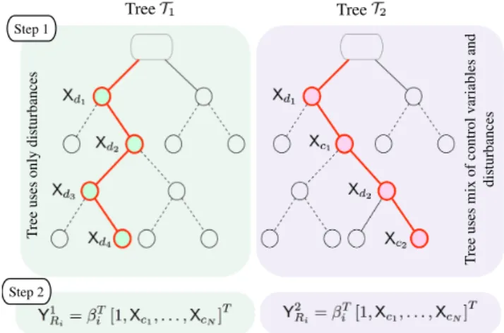
Using separation of variables, the training process is divided into two steps.Step 1: The trees and the ensembles are trained only on Xd_{, which eases the computational}

complexity. It is important to note that besides external disturbances, Xd _{also contains autoregressive terms of the}

output Y which is the main reason for the state space explosion.Step 2:Linear regression models are trained in the leaves (or terminal nodes) of the trees which are function of onlyXc_{. We have validated this linear model assumption in}

[10]. As we shall see in Sec. II-B and II-C, the second step reduces the run-time control problem into a convex program. This process is illustrated in Fig. 1.

B. DPC-RT: DPC with Regression Trees

When the data has lots of features, which interact in com-plicated, nonlinear ways, assembling a single global model such as linear or polynomial regression can be difficult, and can lead to poor response predictions. An approach to non-linear regression is to partition the data space into smaller regions, where the interactions are more manageable. This partition is repeated recursively until finally we get to small chunks of the data space where we can fit simple (eg. linear parametric) models. Therefore, in (1), the global model f

Xd1 Xd2 Xd3 Xd4 Y1 Ri=β T i [1,Xc1, . . . ,XcN] T Tree Y2 Ri=β T i [1,Xc1, . . . ,XcN] T Tree Xd1 T re e us es onl y di st urba nc es T re e us es m ix of c ont rol va ri abl es a nd di st urba nc es Step 1 Step 2

Fig. 1: Separation of variables. Step 1: Tree T1 is trained only

on the disturbances Xd as the features. Tree T2 uses both the

disturbances Xd and the control variablesXc for splitting and is thus not computationally suitable for control.Step 2:In the leafRi of the trees, a linear regression model parametrized byβiis defined as a function only of the control variables.

has two parts: the recursive partition g, and a linear (and convex) modelhfor each cell of the partition.

Now, our goal is to predict the stateYat timekfor nextN

time steps, i.e.Yk+1|k, . . . ,Yk+N|k, whereN is the control

horizon. Applying the separation of variables, we build N

regression trees using CART procedure [2] such that the output Yk+j|k of thejth tree depends upon the previousN

disturbances: Yk+j|k=ftree Xd k+j−N|k, . . . ,Xdk+j−1|k , (2) Xdk+j−l|k∈Rd ∀ l, j= 1, . . . , N.

Then, the linear models as functions of Xc _{in each leaf of}

the tree_Tj are defined as

Yk+j|k =βjT[1,Xck|k, . . . ,Xck+j−1|k]T, (3) Xc

k+j−l|k∈Rc ∀l, j= 1, . . . , N.

Note that the coefficientsβjwould be different for each leaf.

Eq. (3) implies that the prediction of outputYk+j at timek

is an affine combination of control inputs from timektok+

j−1. Thus, we have managed to linearize the original model dynamics via black-box modeling. This two-step training is done offline. In run-time, given the disturbancesXd

k|kat time

k, we can narrow down to a leaf of each tree in (2) to retrieve the linear models in (3).

In run-time, when a new control action is to be determined, each tree (prediction step) contributes to a linear constraint in the optimization as a replacement for the state dynamics in the case of MPC. Thus, the RHC optimization problem with a quadratic cost (_{Q ≥}0,_R0) can be formulated as:

(5)

Here, _{Q ∈} R and R ∈ Rc×c, and the slack variables

j ensure recursive feasibility since the equality constraint

on Y is relaxed. Of course, a different cost function can be chosen depending upon the application. In the current formulation, the data-driven control problem is reduced to a convex program which is much easier to solve than running an optimization directly on a black-box model trained on Xc _{as features. We solve this optimization in the same}

manner as MPC to determine the optimal sequence of inputs

[Xc

k|k, . . . ,Xck+N−1|k], apply the first control input Xck|k and

proceed to the next time step k+ 1. The pseudo code for DPC-RT is given in Alg. 1.

C. DPC-En: DPC with Ensemble Methods

Regression trees obtain good predictive accuracy in many domains. However, the models used in their leaves have some limitations regarding the kind of functions they are able to approximate. The problem with trees is their high variance and that they can overfit the data easily. A small change δ

in the data can result in a different series of splits and thus violate the acceptable accuracyε, i.e._∃Xˆd_{| ||}_Xd₋_X_ˆd_||_{< δ}

&_||Y−Ytrue||> ε. This is the price to be paid for estimating

a tree-based structure from the data.

We use ensemble methods [6] to combine the predictions of several independent regression trees in order to improve generalizability and robustness over a single estimator. The essential idea is to average many noisy trees to reduce the overall variance in prediction. We inject randomness into the tree construction in two ways. First, we randomize the features used to define splitting in each tree. Second, we build each tree using a bootstrapped or sub-sampled data set. In this way, each tree in the forest is trained on different data, which introduces differences between the trees. More explicitly, training features Xd

∈Rp withp < dand the

in-bag samples (in-in-bag samples correspond to the data samples on which the tree was trained) are different for each tree in the forest i.e _|(X,Y)_|< n.

The goal with DPC-En is to replace each tree in Alg. 1 by a forest Yk+j|k=fforest Xdk+j−N|k, . . . ,Xdk+j−1|k , (5) Xdk+j−l|k∈Rp ∀ l, j= 1, . . . , N,

which, again, is trained only on Xd_{, but}_Xd

∈Rp⊂Rd for

each tree, and then fit a linear regression model using Xc

in every leaf of every tree. We build N such forests for N

prediction steps such that the leaf Ri of forest Rj uses a

linear model

Yk+j|k= ΘTij[1,Xck|k, . . . ,Xck+j−1|k]T, (6) Xc_k+j₋_l_|_k_∈Rc ∀l, j= 1, . . . , N.

Here(Xc_,_Y₎_{correspond to the in-bag samples for the trees.}

While the offline training burden in DPC-En is slightly increased compared to DPC-RT, in the control step we exploit the better accuracy, and lower variance properties of the random forest. If a forest hastnumber of trees, given the forecast of disturbances, we havetsets of linear coefficients. We simply average out all the coefficients from all the trees to get one linear model represented byΘˆj for each forest. Note

Algorithm 1Data Predictive Control with Regression Trees

1: DESIGNTIME

2: procedureMODELTRAINING USINGSEPARATION OFVARS

3: SetXc←manipulated features

4: SetXd←non-manipulated features

5: BuildN predictive trees with(Y,Xd₎

defined in (2)

6: for alltreesTjdo

7: for allregionsRiat the leaves ofTj do

8: FitYk+j|k=βjT 1,Xc k|k, . . . ,X c k+j−1|k T as in (3) 9: end for 10: end for 11: end procedure 12: RUNTIME

13: procedurePREDICTIVECONTROL

14: whilek < kstop do 15: for alltreesTj do

16: Determine the leafRiusingXdas in (2)

17: Obtain the linear model atRitrained in (3)

18: end for

19: Solve optimization in (4) to determine optimal

20: control actions[Xck|k, . . . ,X

c

k+N−1|k]

21: Apply the first inputXck|k 22: end while

23: end procedure

that the averaging step can only be done in run-time because the leaf of each tree can be narrowed down only when the Xd _{is known. Thus, for}_N _{forests, we again have exactly}_N

linear equality constraints in the optimization problem below:

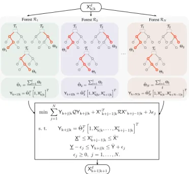
DPC-En is graphically described in Fig. 2. The ensemble data predictive control (DPC-En) is the first such method to bridge the gap between ensemble predictive models (such as random forests) and receding horizon control. In the next section, we compare DPC-RT and DPC-En to MPC for a building model.

III. COMPARISON WITH MPC

We consider a bilinear building model developed at Auto-matic Control Laboratory, ETH Zurich. It captures the essen-tial dynamics governing the zone-level operation while con-sidering the external and the internal thermal disturbances. By Swiss standards, the model used for this study is of a heavyweight construction with a high window area fraction on one facade and high internal gains due to occupancy and equipments [7].

The bilinear model is a standard building model used for practical considerations [12], [15], [16] as it is detailed enough and suitable for model-based control unlike the ones obtained from simulation software like EnergyPlus. We specifically consider this model to show a comparison against MPC. MPC of EnergyPlus models can be cost and time prohibitive, making them unsuitable for control. In Sec. IV, we show how DPC scales easily to such large scale models.

(6)

A. Bilinear Model

The bilinear model has 12 internal states including the inside zone temperature Tin, the slab temperaturesTsb, the

inner wall Tiw and the outside wall temperature Tow. The

state vector is defined asx:= [Tin,T(1:5)_sb ,T(1:3)_ef ,T(1:3)in ]T.

There are 4 control inputs including the blind positionB, the gains due to electric lighting L, the evaporative cooling usage factor C, and the heat from the radiator Hsuch that

u := [B,L,H,C]T_. _B _and _L _{affect both room illuminance}

and temperature due to heat transfer whereasCandHaffect only temperature.

The model is subject to 5 weather disturbances: solar gains with fully closed blindsQscand with open blindsQso,

daylight illuminance with open blinds Io, external dry-bulb

temperature Tdb and external wet-bulb temperature Twb.

The hourly weather forecast, provided by MeteoSwiss, was updated every 12 hrs. Therefore, to improve the forecast, an autoregressive model of the uncertainty was considered. Other disturbances come from the internal gains due to occupancy Qio and due to equipments Qie which were

assumed as per the Swiss standards [14]. We define d := [Qsc,Qso,Io,Qio,Qie,Tdb,Twb]T. For further details, we

refer the reader to [15].

The model dynamics is given below. The bilinearity is present in both input-state, and input-disturbance.

xk+1=Axk+ (Bu+Bxu[xk] +Bdu[dk])uk+Bddk (8)

xk ∈R12, uk ∈R4, dk∈R8 ∀k= 0, . . . , T,

where, the matricesBxu andBdu are defined as

Bxu[xk] = [Bxu,1[xk], Bxu,2[xk], . . . , Bxu,4[xk]]∈R12×4,

Bdu[dk] = [Bdu,1[dk], Bdu,2[dk], . . . , Bdu,4[dk]]∈R12×4,

Bxu,i∈R12×12, Bdu,i∈R12×8 ∀i= 1,2,3,4.

For this study, we assume that the disturbances are precisely known to MPC as well as DPC controller. In our future work, we will account for the uncertainties in the disturbances with an extension to Scenario approach [1] for DPC.

B. Model Predictive Control

We use an MPC controller with a quadratic and a linear cost for comparison. The finite RHC approach involves optimizing a cost function subject to the dynamics of the system and the constraints, over a finite horizon of time [13]. After an optimal sequence of control inputs are computed, the first input is applied, then at the next step the optimization is solved again.

The objective of the controller is to minimize the energy usage cT_u _{while maintaining a desired level of thermal}

comfort. Therefore, at time step k, we solve a continuously linearized MPC problem to determine the optimal sequence

Fig. 2: DPC-En: At time k, the algorithm uses the forecast of disturbances Xdk|k to select linear models Θ1 to Θt in the leaves of each ensemble. The linear models in each ensemble are averaged to calculate a single model represented by Θˆj which act as constraints in the optimization problem. The optimal se-quence[Xck|k, . . . ,X

c

k+N−1|k], of which the first one is applied, and

where _{Q ∈} R12×12 has all zeros except at Q(1,1)

corre-sponding to the zone temperature, c _∈ R4 is proportional

to cost of using each actuator and λ penalizes the slack variables.

C. Data Predictive Control

In this section, we explain how DPC can be applied to this case study. We begin with a description of features X and outputY used for training.

1) Training Data: The fundamental reason why DPC is suitable for such a problem is that when the complexity rises, there is a huge cost to model all the states given by the dynamical system (8). For example, states in the bilinear model also include slab temperatures which require modeling of structural and material properties in detail and often we also need to install new sensors to capture additional states. Thus, DPC is based solely on one state of the model i.e. the zone temperature that can be easily measured with a thermostat. This serves as the output variableY of interest for which we build N trees and N forests as described in Sec. II-B and II-C, respectively. Therefore,Yk+j|k:=x1k+j|k,

(7)

TABLE I: Quantitative comparison of root mean square error (RMSE), R2 _{score, and explained variance (EV) for trees and}

forests for different predictions steps.

RMSE R2 _score _EV

tree-Yk+1|k 0.42 0.75 0.76

tree-Yk+6|k 0.64 0.41 0.42

forest-Yk+1|k 0.29 0.87 0.88 forest-Yk+6|k 0.38 0.78 0.80

where x1 _{is the first component of} _x_{. Next, we define the}

non-manipulated features Xd

k|k. At time k, for the tree Tj

and the forest_Rj, we base these features to include weather

disturbances, external disturbances due to occupancy and equipments, and autoregressive terms of the room tempera-ture, i.e.Xd

k|k:= [dk+j−N|k, . . . , dk+j−1|k, x1k|k, . . . , x1k−δ|k],

whereδ is the order of autoregression. Finally, the inputs in DPC are exactly same as in MPC. i.e.Xc

k+j−1|k:=uk+j−1|k.

The training data in the above format was generated by simulating the bilinear model with rule-based strategies for 10 months in 2007. January and May were deliberately excluded for testing the DPC implementation.

2) Optimization: For a fair comparison with MPC, we cast DPC optimization problem as follows:

Here α = β for DPC-RT and α = ˆΘ for DPC-En. Note that, (10) is DPC analog of (9). The only difference is the state dynamics (9b) and (9c) are now replaced with (10b).

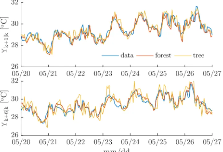
3) Validation: We compare the prediction for the first time step Yk+1|k and the 6-hour ahead prediction Yk+6|k for a

week in the month of May in Fig. 3. It is visible how trees have a high variance, and the forests are more accurate. Note that data from January and May was not used for training. The quantitative summary of the accuracy is given in Tab. I. We can see that the random forests are better in all respects.

D. Comparison

We compare the performance of DPC (10) against an equivalent MPC formulation (9). The solution obtained from MPC sets the benchmark that we compare to. Note that the MPC implementation uses the exact knowledge of the plant dynamics. Therefore, the associated control strategy is indeed the optimal strategy for the plant.

The performance is compared for 3 days in winter, i.e. January 28-31 and 3 days in summer, i.e. May 1-3. These are shown on the same plots in Fig. 4. The sampling time in the simulations is 1 hr. The control horizon N and the order of autoregression are both 6 hrs. The training procedure required a few minutes in the case of trees and 2 hrs for forests on a Win 10 machine with an i7 processor and 8GB memory. The cooling usage factorCis constrained in [0,1],

05/20 05/21 05/22 05/23 05/24 05/25 05/26 05/27 26 28 30 32 Yk + 1 | k [ oC ]

data forest tree

05/20 05/21 05/22 05/23 05/24 05/25 05/26 05/27 mm/dd 26 28 30 32 Yk + 6 | k [ oC ]

Fig. 3: Temperature predictions from a tree and a forest for first step prediction (top) and the 6-hour ahead prediction (bottom). Ensemble method shows a relatively higher accuracy.

the heat input in [0,23] W/m2_{, and the room temperature}

in[19,25]oCduring the winters and[20,26]oCduring the summers. The optimization is solved using CPLEX [8].

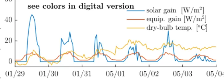
The external disturbances - solar gains, internal gain due to equipment and dry-bulb temperature during the chosen periods are shown in Fig. 4(a). The internal gain due to occupancy was proportional to the gain due to equipment. The reference temperature is chosen to be 22oC. Due to cold weather, which is evident from the dry-bulb temperature, the heater is switched on during the night to maintain the thermal comfort requirements. When the building is occupied during the day, due to excessive internal gains, the building requires cooling. The lighting in the building is adjusted to meet the minimum light requirements. The optimal cooling usage factor and the radiator power for MPC, En and DPC-RT are shown in Fig. 4(b) and Fig. 4(c), respectively. The control strategy with DPC-En shows a remarkable similarity to MPC, switching on/off the equipments at the same time with similar usage. However, the performance with DPC-RT is much different and worse. DPC-RT inherently suffers from high variance which is also evident in the control strategy, thus making it unsuitable for practical purposes. Although it seems like that adding the rate constraints to DPC-En would smoothen its behavior, this was avoided because the sampling time of the system is 1 hr which is already too high. The room temperature profile in Fig. 4(d) is close to the reference in the case of DPC-En as well as MPC. Fig. 4(e) shows that the cumulative cost of the objective function is, as expected, minimum for MPC, and a bit higher for DPC-En. The cost for DPC-RT blows up around 12 noon on 30th January as one of the slack variables is non-zero, which happens due to high model inaccuracy.

The quantitative performance comparison is shown in Tab. II. MPC tracks the reference more closely at the expense of higher input costs in comparison to DPC-En. The higher cost of the inputs in MPC is also due to lighting. DPC-En explains 70.1% variation in the optimal control strategies obtained from MPC while DPC-RT explains only 1.8%. The mean optimal cost of DPC-En is more than MPC, and is maximum for DPC-RT due to a constraint violation.

(8)

TABLE II: Quantitative comparison of explained variance, mean value of objective function, mean input costcTuand mean deviance from the reference temperature|T−Tref|.

explained mean objective mean input mean variance[−] value[−] cost[−] deviance[o_C]

MPC − 22.60 17.16 0.26

DPC-En 70.1% 39.26 15.12 0.48

DPC-RT 1.8% 204.55 16.84 0.57

performance to MPC without using the physical model. However, one major limitation of the bilinear model is that the information about the building power consumption is not available. Much nonlinearities in the system are due to equipment efficiencies which are not considered in the bilinear case but are very important for practical purposes.

Therefore, our next goal is to apply DPC-En on even more complex and realistic EnergyPlus model for which building a model predictive controller is time and cost prohibitive [17]. This is because we would need to model intricate details like the geometry and construction layouts, the equipment design and layout plans, material properties, equipment and operational schedules etc.

IV. APPLICATION: DEMAND RESPONSE In January 2014, the east coast (PJM) electricity grid experienced an 86x increase in the price of electricity from $31/MWh to $2,680/MWh in a matter of 10 minutes. Sim-ilarly, the price spiked 32x from an average of $25/MWh to $800/MWh in July of 2015. This extreme price volatility has become the new norm in our electric grids. Building additional peak generation capacity is not environmentally or economically sustainable. Furthermore, the traditional view of energy efficiency does not address this need for Energy Flexibility. The solution lies with Demand Response (DR) from the customer side - curtailing demand during peak capacity for financial incentives. However, this is a very hard problem for commercial, industrial and institutional plants, the largest electricity consumers.

Thus, the problem of energy management during a DR event makes an ideal case for DPC. In the following sections, we apply DPC-En to a large scale EnergyPlus model to show how effectively DPC can provide a desired power curtailment as well as a desired thermal comfort. DPC builds predictive models of a building based on historical weather, schedule, set-points and electricity consumption data, while also learning from the actions of the building operator. These models are then used for synthesizing recommendations about the control actions that the operator needs to take, during a DR event, to obtain a given load curtailment while providing guarantees on occupant comfort and operations.

A. EnergyPlus Model

We use the DoE Commercial Reference Building (DoE CRB) simulated in EnergyPlus [5] as the virtual test-bed building. This is a large 6 story hotel building consisting of 22 zones with a total area of 122,120 sq.ft. During peak load conditions the building can consume up to 400 kW of power. For the simulation of the DoE CRB building we use actual meteorological year data from Chicago for the years 2012 and 2013. 01/29 01/30 01/31 05/01 05/02 05/03 05/04 0 20 40 60

see colors in digital version

solar gain [W/m2_] equip. gain [W/m2_] dry-bulb temp. [o_C]

(a) External disturances: solar gains, internal gain due to equipment and dry-bulb temperature. 01/290 01/30 01/31 05/01 05/02 05/03 05/04 0.5 1 1.5 co o li n g fa ct o r [ − ] MPC DPC-En DPC-RT

(b) Optimal control input: cooling usage factorCwith0≤C≤1. DPC-En generates a control strategy very simular to MPC.

01/290 01/30 01/31 05/01 05/02 05/03 05/04 10 20 h ea t [W / m 2]

(c) Optimal control input: radiator heatHwith0≤H≤23 W/m2_{. Again,} DPC-En generates a control strategy very simular to MPC.

01/29 01/30 01/31 05/01 05/02 05/03 05/04 mm/dd 16 18 20 22 24 26 28 ro o m te m p . [ oC ]

(d) Room temperature has time varying bounds. When the building is occuped the constraints are relaxed, else19(20)≤Tin ≤25(26)oCin January(May). MPC and DPC-En are able to track the reference temperature (22oC) closely. 01/290 01/30 01/31 05/01 05/02 05/03 05/04 5000 cu m . co st

(e) Cumulative optimal cost after solving optimization. MPC serves as the benchmark with the minimum cost, followed by DPC-En and then DPC-RT.

Fig. 4: Comparison of optimal performance obtained with MPC, DPC-En and DPC-RT for 3 days in January and 3 days in May.

B. Model training for DPC

In the following simulations, we consider a long DR event from 7am - 2pm when the end-users are expected to follow/track the reference power signal sent by the utility. This is indeed common in Demand Tracking Control. During offline training, we sample data every 15 min to learn 2 kinds of forests. (1) Power forests are built using output as

(9)

the total building power consumption, and (2) Temperature forests with output as temperature of one of the 22 zones.

The training data set contains the following types of features. (1) Theweather datawhich includes measurements of the outside air temperature and relative humidity. Since we are interested in predicting the power consumption or the zone temperature for a finite horizon, we include the weather forecast of the complete horizon in the training features. (2) The schedule data includes the proxy variables which cor-relate with repeated patterns of electricity consumption e.g., due to occupancy or equipment schedules. Day of Week is a categorical predictor which takes values from 1-7 depending on the day of the week. This variable can capture any power consumption patterns which occur on specific days of the week. Likewise, Time of Day is quite an important predictor of power consumption as it can adequately capture daily patterns of occupancy, lighting and appliance use without directly measuring any one of them. Besides using proxy schedule predictors, actual building equipment schedules can also be used as training data for building the trees. (3) The

building data include (i) cooling set points for the guest rooms, kitchen and corridors, (ii) supply air temperature, and (iii) chilled water temperature.

For the following simulations, we use five control variables (i) cooling set point for corridorsClgSP, (ii) cooling set point for guest roomsGuestSP, (iii) cooling set point for kitchen KitchenSP, (iv) chilled water supply temperature ChwSP, and (v) supply air temperature SupplyAirSP, so Xc ₌ [ClgSP,GuestClgSP,KitchenClgSP,SupplyAirSP,ChwSP]. The power forest _Rp is built using the total building

power consumption P. Its features Xd _{include the weather}

variables, their lag terms and their forecast over the horizon, the schedule variables, and finally the lag terms of the power consumption. The temperature forest _Rt is built

with zone temperature T as the output. Except for the lag terms corresponding to the same zone temperature, all other features are same inXd_.

Fig. 5 shows the prediction accuracy for the power forest, and also explains the two level training approach introduced in Sec. II-A. During S1, the forests are trained using only disturbances as the features. Then in S2, the local effects of the control variables are accounted for by the linear models in the leaves. We observe how the accuracy is drastically improved after including the linear models in the predictions.

0:00 4:00 8:00 12:00 16:00 20:00 0:00 4:00 8:00 12:00 16:00 20:00 time [hh:mm] 0 50 100 150 200 250 300 350 400 450 pow er c ons um pti on [kW ]

true forest + linear model only forest

Fig. 5: Model accuracy during training: The prediction made by forest using onlyXd(red) captures the effect due to disturbances. The linear models in the leaves capture the local effects (green) due to the control inputsXcand improve the model accuracy.

1:00 3:00 5:00 7:00 9:00 11:00 13:00 15:00 17:00 19:00 21:00 23:00 time [hh:mm] 5 10 15 20 25 30 tem pe rat ure [de g C] ClgSP KitchenClgSP GuestClgSP SupplyAirSP ChwSP

(a) Optimal inputs calculated by DPC-En. At first, the inputs are changed rapidly because of a significant difference between the desired and the actual power consumption. Then gradual adjustments are made to follow the desired reference.

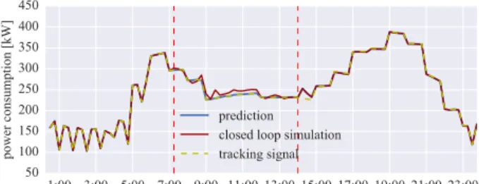
1:00 3:00 5:00 7:00 9:00 11:00 13:00 15:00 17:00 19:00 21:00 23:00 time [hh:mm] 50 100 150 200 250 300 350 400 450 pow er c ons um pti on [kW ] prediction closed loop simulation tracking signal

(b) Power tracking by DPC-En at 1.1 MW: The difference in closed-loop simulation and prediction is due to model mismatch.

Fig. 6: Power management using DPC. The controller is active between 7am - 2pm. This region is marked in dashed red lines.

C. Power Management

Typically, the end customer receives a notification to curtail the power by some fraction. In this example on power management, we show how DPC can generate optimal inputs to track a desired power signal within a small allowance while maintaining the zone level thermal comfort. It may not be possible to have the same thermal comfort level in all the zones due to power curtailment, so we choose one zone (for example CEO’s office) where the constraints must be met. This is done by solving the following optimization problem with control variablesXc₌ [ClgSP,GuestClgSP,KitchenClgSP,SupplyAirSP,ChwSP]

Here, the temperature forests are used to enforce thermal constraints in the zone of interest. The setup of optimization problem is flexible to include even other variables in the cost or the constraints. For example, we are currently looking at including the dynamic pricing of electricity in the cost since the customers can more directly relate to the financial incentives.

The results are shown in Fig. 6. The DPC controller is active between 7am - 2pm. Before 7am and after 2pm, the

(10)

building is using a predefined rule-based control strategy. The optimal control inputs from DPC-En are shown in Fig. 6(a). It is observed that, with the optimal inputs generated by DPC, we can track the reference power consumption signal closely. In fact, the average tracking error between 7am - 2pm is 3%. The difference between the predicted power consumption and that in the closed-loop simulation in Fig. 6(b) is due to model mismatch between the EnergyPlus model and the power forest used in the optimization (11). Due to this inaccuracy, the actual power consumption is on an average 7 kW higher. Thus, DPC-En successfully tracks a given power reference signal with an average _∼ 3% error for such a complex building which would require several years of efforts to develop a physics based model.

D. Practical Challenges and Future Work

Data Availability:The main practical challenge for DPC lies in the availability of data for training and we require answers to questions like how much data (functional testing) is required, and how should the sampling be done? Therefore, the procedure for optimal experiment design, and model improvement with estimation of variance in predictions is one of the main focus of our ongoing work.

Stability:While the buildings are inherently stable, many other applications require stability guarantees. In our ongoing work, we are working towards proving asymptotic stability to origin with DPC-RT and DPC-En by using concept of switched LTI systems. This will make DPC useful for systems with faster dynamics.

Robustness: Another direction of work is on handling uncertainties in the DPC framework, namely an extension to Scenario DPC to account for the disturbance uncertainty. This will help us in quantifying the robustness of DPC.

V. CONCLUSION

We present two algorithms based on trees and random forests for receding horizon control with data-driven models. We compare the performance of our Data Predictive Control to MPC on a multivariable bilinear building model. We establish that DPC with random forests shows a remarkable similarity to MPC in the optimal control strategies explaining 70% variance. On the other hand, DPC with regression trees suffers from practical limitations due to model overfitting. We further apply DPC with random forests to a large scale 6 story EnergyPlus model with 22 zones for which the traditional model-based control is largely unsuitable due to complex dynamics and the cost of model identification. We show that DPC, relying only on the sensor data, can provide significant energy savings while maintaining thermal comfort. Our results demonstrate that even for such complex system, DPC tracks a reference signal with a mean error of 3%.

DPC has applications which go beyond buildings and energy systems, to industrial process control, and controlling large critical infrastructures like water networks, district heating & cooling. DPC is immensely valuable in situations where first principles based modeling cost is extremely high.

ACKNOWLEDGMENT

The authors would like to thank Xiaojing Zhang, a Post-Doctoral Researcher at the University of California, Berkeley for providing the building model, and Manfred Morari for his feedback on DPC.

REFERENCES

[1] D. Bernardini and A. Bemporad. Scenario-based model predictive con-trol of stochastic constrained linear systems. InDecision and Control, 2009 held jointly with the 2009 28th Chinese Control Conference. CDC/CCC 2009. Proceedings of the 48th IEEE Conference on, pages 6333–6338. IEEE, 2009.

[2] L. Breiman, J. Friedman, C. J. Stone, and R. A. Olshen.Classification and regression trees. CRC press, 1984.

[3] D. B. Crawley, L. K. Lawrie, F. C. Winkelmann, W. F. Buhl, Y. J. Huang, C. O. Pedersen, R. K. Strand, R. J. Liesen, D. E. Fisher, M. J. Witte, et al. Energyplus: Creating a new-generation building energy simulation program. Energy and buildings, 33(4):319–331, 2001. [4] D. Davis. Lighting the Way to Demand Response Lighting the Way

to Demand Response. Technical report, CEC, 2011.

[5] M. Deru, K. Field, D. Studer, K. Benne, B. Griffith, P. Torcellini, B. Liu, M. Halverson, D. Winiarski, M. Rosenberg, et al. Us department of energy commercial reference building models of the national building stock. 2011.

[6] J. Friedman, T. Hastie, and R. Tibshirani.The elements of statistical learning, volume 1. Springer series in statistics Springer, Berlin, 2001. [7] D. Gyalistras and M. Gwerder. Use of weather and occupancy forecasts for optimal building climate control (opticontrol): Two years progress report main report. Terrestrial Systems Ecology ETH Zurich R&D HVAC Products, Building Technologies Division, Siemens Switzerland Ltd, Zug, Switzerland, 2010.

[8] I. ILOG. IBM ILOG CPLEX Optimizer-Highperformance mathe-matical programming solver for linear programming, mixed integer programming, and quadratic programming, 2012.

[9] A. Jain, M. Behl, and R. Mangharam. Data Predictive Control for building energy management. InProceedings of the 2017 American Control Conference. IEEE, 2017.

[10] A. Jain, R. Mangharam, and M. Behl. Data Predictive Control for peak power reduction. InProceedings of the 3rd ACM International Conference on Systems for Energy-Efficient Built Environments, pages 109–118. ACM, 2016.

[11] A. Kusiak, Z. Song, and H. Zheng. Anticipatory control of wind turbines with data-driven predictive models. IEEE Transactions on Energy Conversion, 24(3):766–774, 2009.

[12] Y. Ma, J. Matuˇsko, and F. Borrelli. Stochastic Model Predictive Control for building hvac systems: Complexity and conservatism.

IEEE Transactions on Control Systems Technology, 23(1):101–116, 2015.

[13] D. Q. Mayne, J. B. Rawlings, C. V. Rao, and P. O. Scokaert. Con-strained model predictive control: Stability and optimality.Automatica, 36(6):789–814, 2000.

[14] S. Merkblatt. 2024: Standard-nutzungsbedingungen für die energie-und gebäudetechnik. Zürich: Swiss Society of Engineers and Archi-tects, 2006.

[15] F. Oldewurtel.Stochastic Model Predictive Control for energy efficient building climate control. PhD thesis, ETH Zurich, 2011.

[16] F. Oldewurtel, A. Parisio, C. N. Jones, D. Gyalistras, M. Gwerder, V. Stauch, B. Lehmann, and M. Morari. Use of Model Predictive Control and weather forecasts for energy efficient building climate control. Energy and Buildings, 45:15–27, 2012.

[17] D. Sturzenegger, D. Gyalistras, M. Morari, and R. S. Smith. Model predictive climate control of a swiss office building: Implementation, results, and cost–benefit analysis. IEEE Transactions on Control Systems Technology, 24(1):1–12, 2016.

[18] E. ˇZáˇceková, Z. Váˇna, and J. Cigler. Towards the real-life implemen-tation of MPC for an office building: Identification issues. Applied Energy, 135:53–62, 2014.