Efficient Analysis of
Complex Changepoint
Problems
Robert Maidstone
Submitted for the degree of Doctor of Philosophy at
Lancaster University.
Abstract
Many time series experience abrupt changes in structure. Detecting where these changes in structure, or changepoints, occur is required for effective modelling of the data. In this thesis we explore the common approaches used for detecting changepoints. We focus in particular on techniques which can be formulated in terms of minimising a cost over segmentations and solved exactly using a class of dynamic programming algorithms. Often implementations of these dynamic programming methods have a computational cost which scales poorly with the length of the time series. Recently pruning ideas have been suggested that can speed up the dynamic programming algorithms, whilst still being guaranteed to be optimal.
In this thesis we extend these methods. First we develop two new algorithms for segmenting piecewise constant data: FPOP and SNIP. We evaluate them against other methods in the literature. We then move on to develop the method OPPL for detecting changes in data subject to fitting a continuous piecewise linear model. We evaluate it against similar methods. We finally extend the OPPL method to deal with penalties that depend on the segment length.
Acknowledgements
Firstly I would like to thank everyone involved with the Statistics and Operational Research Centre for Doctoral Training at Lancaster University, especially the leadership team Jon Tawn, Idris Eckley and Kevin Glazebrook for giving me the opportunity to be part of the unique, stimulating research environment which STOR-i provides. I am also very grateful for the financial support provided through STOR-i by the EPSRC, and hope they continue to fund similar projects in the future.
The work in Chapter 3 is taken from the paper Maidstone et al. (2016) and I would like to thank my collaborators on this work; Guillem Rigaill and Toby Hocking. Discussions on this paper first started during the workshopInference for Change-Point and Related Processes at the Isaac Newton Institute for Mathematical Sciences in Cambridge, and I would like to thank them for their support and hospitality. Further insightful emails with Guillem and Toby (and a productive meeting with Guillem in Lancaster) proved valuable in the development of the paper and Guillem and Toby’s coding and analysis of the FPOP algorithm was also invaluable.
Perhaps most importantly, I would like to thank my supervisors Adam Letchford and Paul Fearnhead for all the time and effort they have put into this PhD project. Not only have they taught me a lot about the technical and statistical methods discussed in this thesis, but I feel that I have also learnt valuable research and life skills under their guidance.
The students of STOR-i over the years I have been part of the programme also deserve a mention as they have all impacted my life positively. In particular my intake year Emma, Ben, Dave, Judd, Tom, Hugo, Jeddy and Rhian have provided much friendship and banter as well as the occasional in-depth discussion. Lastly I would like to thank Kaylea for putting up with me and doing a lot of proof reading.
Declaration
I declare that the work in this thesis has been done by myself and has not been submitted elsewhere for the award of any other degree.
Robert Maidstone
Contents
1 Introduction 1
2 Literature Review 3
2.1 Detecting a Single Changepoint . . . 4
2.1.1 CUSUM . . . 4
2.1.2 Likelihood-Ratio Based Approach . . . 5
2.1.3 Penalised Likelihood . . . 6
2.1.4 Bayesian Methods . . . 7
2.2 Multiple Changepoint Methods . . . 8
2.2.1 Binary Segmentation . . . 8
2.2.2 Dynamic Programming Based Methods . . . 12
2.2.3 Bayesian Methods . . . 15
2.2.4 Fused LASSO . . . 20
2.2.5 Simultaneous Multiscale Change-Point Inference . . . 21
2.3 Nonparametric Methods . . . 22
2.4 Fitting More Complex Models . . . 24
2.4.1 Autoregressive Processes . . . 24
2.4.2 Multivariate Data . . . 27
3 On Optimal Multiple Changepoint Algorithms for Large Data 30 3.1 Introduction . . . 30
3.2 Model Definition . . . 32
3.2.1 Segmenting Data using Penalised and Constrained Optimisation . . . 33
CONTENTS V
3.2.2 Conditions for Pruning . . . 35
3.3 Solving the Penalised Optimisation Problem . . . 36
3.3.1 Optimal Partitioning . . . 36
3.3.2 PELT . . . 37
3.4 Solving the Constrained Optimisation Problem . . . 38
3.4.1 Segment Neighbourhood Search . . . 38
3.4.2 Pruned Segment Neighbourhood Search . . . 39
3.5 New Changepoint Algorithms . . . 43
3.5.1 Functional Pruning Optimal Partitioning . . . 43
3.5.2 Segment Neighbourhood with Inequality Pruning . . . 46
3.6 Comparisons Between Pruning Methods . . . 48
3.7 Empirical evaluation of FPOP . . . 50
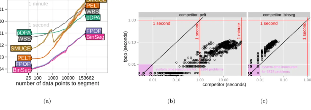
3.7.1 Speed benchmark: 4467 chromosomes from tumour microarrays . . . 51
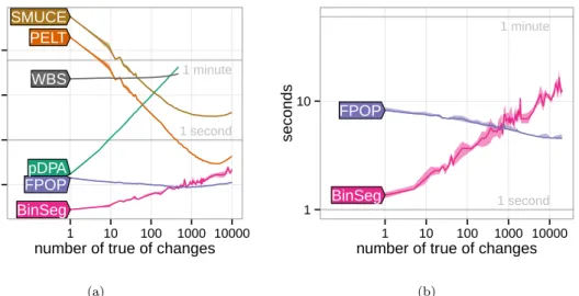
3.7.2 Speed benchmark: simulated data with different number of changes . . . 52
3.7.3 Accuracy benchmark: the neuroblastoma data set . . . 53
3.7.4 Accuracy on the WBS simulation benchmark . . . 55
3.8 Discussion . . . 56
4 Optimal Changepoint Detection for Piecewise Linear Data 60 4.1 Introduction . . . 60
4.2 Model Definition . . . 63
4.3 Optimal Partitioning for Piecewise Linear Data . . . 65
4.3.1 Dynamic Programming Approach . . . 65
4.3.2 Functional Pruning . . . 67
4.3.3 Inequality Based Pruning . . . 70
4.4 Evaluation of the Algorithm . . . 72
4.4.1 Empirical Evaluation of the Computational Time . . . 72
4.4.2 Comparison with other methods . . . 76
4.5 Detecting Changes in the Rotation of Bacterial Flagellar Motors . . . 80
CONTENTS VI
5 OPPL for Penalties which Depend on the Segment Length 92
5.1 Introduction . . . 92
5.2 Penalised Cost with General Penalty Function . . . 93
5.3 OPPL with a Penalty that Depends on the Segment Length . . . 93
5.3.1 Functional Pruning . . . 94
5.3.2 Inequality Based Pruning . . . 96
5.4 Comparing OPPL with the mBIC penalty to OPPL with the BIC penalty . . . 97
5.5 Discussion . . . 100
6 Discussion 105 6.1 Summary of the Contribution of the Thesis . . . 105
6.2 Future Directions . . . 108
6.2.1 Expanding FPOP to a more complex cost functions . . . 108
6.2.2 Expanding OPPL to a larger class of models . . . 109
6.2.3 Confidence Bounds . . . 111
7 Appendix 112 A Further Simulation Results from Chapter 3 113 A.1 Short Description of the WBS Benchmark Scenarios . . . 113
A.2 Accuracy Results for WBS Benchmark Scenarios . . . 114
A.3 Accuracy Results for Speed Simulations . . . 117
B Coefficient updating for OPPL using a Normal likelihood cost function 121 B.1 Coefficient Updating for OPPL with a Penalty Function which Depends on the Segment Length . . . 122
List of Figures
1.1 Example of data with sudden changes in structure . . . 2
2.1 Plot of the unpenalised cost against the number of segments found . . . 16
2.2 Hidden Markov model topology . . . 20
3.1 pDPA cost functions for a change in mean using the negative normal log-likelihood cost function. . . 41
3.2 Stored functions by the pDPA algorithm over 2 time steps . . . 42
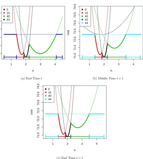
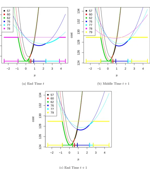
3.3 Stored functions by the FPOP algorithm over 2 time steps . . . 47
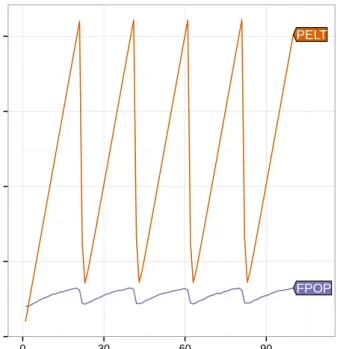
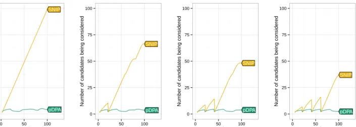
3.4 Comparison of the number of candidate changepoints stored over time by FPOP and PELT. 48 3.5 Comparison of the number of candidate changepoints stored over time by pDPA and SNIP. 49 3.6 Timings on the tumour microarray benchmark. . . 53
3.7 Runtimes in simulated data sets with a variable number of true changepoints . . . 54
3.8 Accuracy results on the neuroblastoma data set. . . 56
4.1 Example of piecewise linear data . . . 61
4.2 Subsection of data showing the rotation of a bacterial flagellar motor over time. . . 62
4.3 Length of the sets of changepoint vectors stored in OPPL for data with 19 true changes . 75 4.4 Length of the sets of changepoint vectors stored in OPPL for data with no changes . . . . 75
4.5 Computational time taken by the OPPL algorithm. . . 76
4.6 Comparison of changepoint detection methods for piecewise linear data for a linearly increasing number of changes . . . 84
LIST OF FIGURES VIII
4.7 Comparison of changepoint detection methods for piecewise linear data for a constant number of changes . . . 85 4.8 Mean squared error and number of changepoints detected as the parameter changes in
OPPL and Trend Filtering for a data set with randomly drawn values at the changes . . . 86 4.9 Mean squared error and true positive and false positive counts as the parameter changes
in OPPL and Trend Filtering for a data set with randomly drawn values at the changes . 86 4.10 Examples of fit given by OPPL and Trend Filtering. . . 87 4.11 Mean squared error and number of changepoints detected as the parameter changes in
OPPL and Trend Filtering for the saw tooth data set . . . 87 4.12 Mean squared error and true positive and false positive counts as the parameter changes
in OPPL and Trend Filtering for the saw tooth data set . . . 88 4.13 The rotation of a bacterial flagellar motor over time with the estimate given by using a
Potts functional . . . 88 4.14 The rotation of a bacterial flagellar motor over time with the estimate given by OPPL . . 89 4.15 The unpenalised cost for the piecewise constant and piecewise linear models as the number
of parameters increases. . . 89 4.16 Histograms and scatter plot of the absolute gradient and the length of the segments in
the optimal segmentation found by OPPL. . . 90 4.17 Analysis of the dwell regions . . . 91
5.1 Length of the sets of changepoint vectors stored for data with 19 true changes . . . 99 5.2 Comparison of OPPL with the BIC and mBIC penalties for a linearly increasing number
of changes . . . 101 5.3 Comparison of OPPL with the BIC and mBIC penalties for a constant number of changes 102 5.4 Comparison of OPPL with the BIC and mBIC penalties for a linear number of randomly
List of Algorithms
1 Binary Segmentation . . . 9
2 Functional Pruning Optimal Partitioning (FPOP) . . . 58
3 Segment Neighbourhood with Inequality Pruning (SNIP) . . . 59
4 Algorithm for Optimal Partitioning of Piecewise Linear Data (OPPL) . . . 73
5 Algorithm for calculation of Intt τ at time t . . . 74
6 Algorithm for OPPL with a penalty that depends on the segment length . . . 98
Chapter 1
Introduction
Analysis of time series data is required in numerous applications including finance (Fryzlewicz, 2014), medical statistics (Lavielle, 2005), climatology (Killick et al., 2010) and technology (Lung-Yut-Fong et al., 2012). As data collection and storage methods improve, these data sets are getting increasingly bigger. This has led to the idea of Big Data (B¨uhlmann et al., 2016). Big Data refers to data sets that are so huge that traditional statistical and analytical techniques cannot be applied, due to the exorbitant computational resources (time and/or memory) that would be needed. To analyse such data sets, new models and/or algorithms are required.
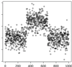
One area which requires algorithms to deal with Big Data is changepoint detection in time series. Changepoint models are often fitted to time series to deal with scenarios where the data experiences a sudden change in structure, such as that shown in Figure 1.1. These changes in structure, known as changepoints or breakpoints need to be taken into account if the data is to be modelled effectively.
The structure of this thesis is as follows. In Chapter 2 we will discuss some of the large body of liter-ature on changepoint detection including; detection of a single change, multiple changepoint detection, Bayesian methods, nonparametric methods, multivariate methods and methods for more complicated data structures.
Then in Chapter 3 we will extend the discussion to pruned dynamic programming methods and develop two methods of our own; Functional Pruning Optimal Partitioning (FPOP) and Segment Neigh-bourhood with Inequality Pruning (SNIP). We evaluate the algorithms against competing methods and apply the FPOP algorithm to detecting changes in DNA copy number data in tumour microarray data.
CHAPTER 1. INTRODUCTION 2 0 200 400 600 800 1000 −4 −2 0 2 4 6 Time yt
Figure 1.1: Example of data with sudden changes in structure. In this case a change in mean.
Chapter 4 considers the problem of fitting a piecewise linear model to the data where at the change-points (places where the trend changes) we enforce continuity. Such a model is often of interest, for example when considering changes in velocity. We develop a method, Optimal Partitioning for Piecewise Linear data (OPPL), based on a dynamic programming algorithm with pruning steps added to it. We evaluate the method in terms of both efficiency and accuracy. We then apply the method to detecting changes in the angular velocity of a biological motor.
Chapter 5 offers an extension to the OPPL algorithm, adapting it to work with a penalty func-tion which depends on the lengths of the fitted segments. Again this method is evaluated in terms of the efficiency and the accuracy and compared to using the standard OPPL method with the Bayesian Information Criterion (BIC) penalty value, which depends only on the length of the data set.
Finally, in Chapter 6, we conclude with a discussion of the main contributions of the thesis and potential paths to extend the methods developed in the future.
Chapter 2
Literature Review
The literature on changepoint detection is large and in this chapter we will discuss some of the key contributing papers. For a general overview of changepoint methods we refer the reader to the books Carlstein et al. (1994) and Chen and Gupta (2011), the book chapter Eckley et al. (2011) and the review papers Braun and M¨uller (1998) and Reeves et al. (2007).
We assume that we have data ordered by time, or some other attribute such as position along a chromosome. We denote this data byy= (y1, . . . , yn). We are then interested in detecting the existence
of changes in the structure of the data. We denote the number of changes asmand the positions of the changes byτ = (τ1, . . . , τm), labelled such thatτ1 < τ2 < . . . τm. Often this is extended to letτ0 = 0
andτm+1=n. In this section we discuss techniques for detecting changes in such data.
Often changepoint detection can be thought of in terms of two concepts. First we define some criterion on the data for model selection. This could be a cost to be minimised, such as the negative log likelihood, or a test statistic, such as the CUSUM. Secondly we require a search algorithm to find the changepoint (and segment parameter) estimates that satisfy the criterion.
In this literature review we will consider examples of both. First in Section 2.1 we consider detecting a single changepoint. These methods often do not require a search algorithm as checking every single changepoint location individually is usually feasible. In Section 2.2 we move on to consider multiple changepoint detection. In these methods checking all solutions is infeasible for large data sets and hence novel search algorithms are required.
CHAPTER 2. LITERATURE REVIEW 4
2.1
Detecting a Single Changepoint
The detection of single changepoints can be useful for a number of reasons. For example, even when multiple changepoints exist, proving the existence of a single change in the structure can be enough to highlight the flaws in current models which assume no such changes exist.
The problem of detecting a single changepoint is fairly straight forward, and comes down to a model selection problem; whether to choose the model withm= 0 or the model withm= 1 with a changepoint at some location,τ. Four types of methods will be discussed here; the CUSUM test statistic, a likelihood-ratio based approach, penalised likelihood methods and Bayesian methods.
2.1.1
CUSUM
A simple method for single changepoint detection is to use a test statistic based on the cumulative sums of the data. This test statistic, known as the CUSUM test statistic, was first considered for changepoint detection problems in Page (1954) where a change in mean was considered. The CUSUM for a change in mean of an i.i.d. time series,y1, . . . , yn, is then defined as
Un(bnrc) =n− 1 2 bnrc X i=1 (yi−y¯n),
where r∈[0,1] and ¯yn is the sample mean of the sequence. The idea is if a changepoint occurs then
the CUSUM will get large, if no changepoint occurs then the values either side of the mean will cancel each other out and the CUSUM test statistic will remain small. Un can be shown to converge weakly
to a standard Brownian bridge and this convergence result can be used to provide a suitable threshold value to test against.
Similar results can be shown for more general cases and as such the CUSUM provides a simple test for changepoint detection. Changes in regression are considered in Brown et al. (1975), where they also consider a related test statistic based on the sum of the squares of the data. Extensions of the CUSUM to changes in variance were considered in Inclan and Tiao (1994). Detecting a change in an autoregressive models is also considered by a number of authors including Lee et al. (2003) for an AR(1) process, Zhou and Liu (2009) for a change in mean in an infinite variance AR(p) process and Bai (1994) for detecting changes in ARMA models.
CHAPTER 2. LITERATURE REVIEW 5
2.1.2
Likelihood-Ratio Based Approach
When it comes to model selection between two competing methods, one solution which instantly comes to mind is the likelihood-ratio test, which was first proposed for changepoint models by Hinkley (1970). This is used to compare the fit of two models where one (the null) is nested inside the other (the alternative). This is clearly the case in the situation of detecting a single changepoint, as the model where there is no changepoint is just a special case (where the two segment models are identical) of the model with a single changepoint. Hence we can define the null and alternative hypotheses as follows:
H0: No changepoint,m= 0,
H1: A single changepoint,m= 1.
H1 then corresponds to a model with a single changepoint atτ∈(2,3, . . . , n−1).
Assume that a single model with density p(y1:n|θ) is fitted to the null model and that the two
modelsp1(y1:τ|θ1) andp2(yτ:n|θ2) are fitted to the alternative. Then to use the likelihood-ratio test the
likelihood-ratio test statistic, or equivalently the log-likelihood-ratio test statistic, needs to be calculated. The log-likelihood-ratio test is calculated as follows;
W(τ) =−2 log LH0(θˆ) LH1(θ1ˆ ,θ2ˆ) , =−2 log Qn i=1p(yi|θˆ) Qτ i=1p1(yi|θ1ˆ)Q n i=τp2(yi|θ2ˆ) , = 2 " τ X i=1 logp1(yi|θ1ˆ) + n X i=τ+1 logp2(yi|θ2ˆ)− n X i=1 logp(yi|θˆ) # .
However this only works ifτ is known, this is almost certainly not the case. To calculate the likelihood-ratio test statistic for unknownτ, we then need to take the maximum over all possible values ofτ
W = max
τ W(τ).
Then the null hypothesis (that there is no changepoint) is rejected in favour of the alternative (there is a single changepoint) ifW > cwherecis some threshold value.
This threshold value is often taken to be csuch thatα= Pr(W > c|H0 is true) for some significance
levelα. The standard approach for the likelihood-ratio test is to assume thatW is distributed with aχ2
d∗
distribution (whered∗ is the difference in the number of parameters), this is known as Wilks’ Theorem (Wilks, 1938). However this result does not hold for the changepoint problem as, due to the parameter τ being discrete, the two models are not considered “nested” under Wilks’ assumptions.
CHAPTER 2. LITERATURE REVIEW 6
Yao and Davis (1986) derive the null distribution for a changepoint model with a change in mean in Normal random variables as converging in distribution to the double exponential extreme value distribu-tion. They also give a more precise finite-sample approximadistribu-tion. Using either of these,c can be chosen as the (1−α)×100% quantile of the distribution.
Examples of the likelihood-ratio test statistic being used to detect single changepoints can be found in a number of papers. Notable examples include Hinkley (1970), where it is used on normally distributed data with a change in mean and Haccou et al. (1987) where the test is applied to exponentially distributed data with a change in the rate parameter (which affects both the mean and variance of the distribution).
2.1.3
Penalised Likelihood
Another way of detecting a single changepoint is to use the penalised likelihood. Fitting a penalised likelihood model is considered in the case of multiple changepoints, however the methodology can be applied to single changepoint detection. The likelihood is used as a measure of fit with an added penalty term to avoid overfitting. The likelihood and penalty term are combined into a single function which is then minimised. If we consider fitting a modelM, withpparameters. Denote the parameters byθ and the likelihood byL(θ). The penalised likelihood is then defined as
P L(M) =−2 log maxL(θ) +pβ,
whereβis a penalty parameter which often depends on the data lengthn. The modelMthat minimises P L(M) is then the preferred model.
For changepoint detection we search over all models with 0 or 1 changes, the total number of param-eters is then eitherp= “number of parameters for modelling as a single segment” or p= 1+ “number parameters for modelling as two segments” respectively.
The penalised likelihood is similar in theory to running a log-likelihood test as both methods will prefer a model with one changepoint if the increase in the log-likelihood is greater than a constant. For the penalised likelihood this constant is related to the penalty term,β. The method is highly dependent on the choice of this penalty term and the choice of this will be discussed further in Section 2.2.2.
CHAPTER 2. LITERATURE REVIEW 7
2.1.4
Bayesian Methods
If, when considering changepoint models, prior information on the parameters is known (or assumed) then Bayesian techniques can be of use. Priors can be chosen for the individual segment parameters, (θ, θ1, θ2), the number of changepoints, m ∈ {0,1}, and the locations of the potential changepoint, τ.
Using these, posteriors can be calculated and the optimal model can be selected as the one with the largest posterior probability. A mathematical formulation of this is now given.
Letp(θ|ψ) denote the prior on the parametersθ, whereψ are hyperparameters. Then the segment marginal likelihood can be defined by:
Q(s, t|ψ) =
Z
p(ys:t|θ)p(θ|ψ) dθ. (2.1)
Next assume that a prior probability for the existence of a changepoint is specified, that isP r(M = 1) is given. Then obviously the probability for there being no changepoints is also given, P r(M = 0) = 1−P r(M = 1). Also assign a prior to the changepoint location,τ, and denote this byp(τ). Then, for the case in which theψ are known, the posterior probabilities can be found as follows:
P r(M = 0|y1:n)∝P r(M = 0)Q(1, n|ψ),
P r(M = 1|y1:n)∝P r(M = 1)p(τ)Q(1, τ|ψ)Q(τ+ 1, n|ψ), (forτ= 1, . . . , n).
These values can be calculated inO(n) time, and they can be easily normalised to give the exact posterior probabilities.
To grade the decisiveness of the evidence in favour of selecting one model over another the Bayes Factor can be used. This is defined as the ratio of the posterior odds over the prior odds. Jeffreys (1961) gives a guide on how to use the Bayes Factor.
In some cases the integral in (2.1) is intractable and cannot be computed. One solution to this is to use MCMC to simulate from the marginal posterior distribution. Carlin et al. (1992) give an example of this where they use the Gibbs sampler to detect a single change in a Poisson process. They further apply their method to detecting a single change in the observations from a Markov chain and an simple linear regression.
CHAPTER 2. LITERATURE REVIEW 8
2.2
Multiple Changepoint Methods
Single changepoint detection methods can often be extended to the multiple changepoint detection case, however the multiple changepoint case is much more computationally challenging. For a data set of length n, rather than havingn−1 potential positions for a changepoints we have 2n−1 sets of possibilities to
check if the number of changepoints is unbounded. Due to this added complexity novel search methods are required to efficiently compute solutions.
2.2.1
Binary Segmentation
Binary Segmentation, first introduced in Scott and Knott (1974) (and first used in a stochastic setting in Vostrikova (1981)), is one of the most widely used changepoint detection methods. This is due to its simplicity, fast runtime and relatively good accuracy.
Binary Segmentation takes a recursive approach. The idea is that if a single changepoint can be detected in a time series then the series can be split around this changepoint into two sub-series either side of the change. Then the single changepoint detection method can be applied to each of the sub-series. This can then be iterated until no further changepoints are detected.
Often this is achieved via the calculation of a test statistic, Γ(y1:n), that is dependent on the data.
This test statistic can be computed over the full data set and then compared to a threshold value,c, to determine if a change occurs. If it does then the change is calculated via an estimator ˆτ(y1:n) and stored.
The data is then split around this detected changepoint and the process is repeated on the two subsets of the data y1:ˆτ(y1:n) and yˆτ(y1:n)+1:n. This process is repeated until the threshold is not breached by
any subset of the data. The stored changepoints are then returned.
An obvious choice for the test statistic is to use the likelihood-ratio test (from Section 2.1.2). With the null hypothesis corresponding to the model with no changepoint and the alternative with a change at timeτ ∈(1,2, . . . , n−1) then we can define a test statistic Γ on the segment fromstotas follows
Γ(ys:t) = 2 " max τ τ X i=s logp1(yi|ˆθ1) + t X i=τ+1 logp2(yi|θ2ˆ ) ! − t X i=s logp(yi|ˆθ) # .
The null hypothesis is rejected in favour of the alternative (i.e. we detect a changepoint) if Γ(ys:t)> c
for some threshold valuec to be chosen. Often this value is chosen to be such thatα=P r(Γ(ys:t)>
CHAPTER 2. LITERATURE REVIEW 9
maximises the test statistic. One issue with using the likelihood-ratio test in this way is that at each stage of the algorithm we test for the existence of a changepoint by comparing against the null hypothesis that no such change exists, even though we may already know of the existence of a change. Hyun et al. (2016) discusses the issues with this naive approach further and offers an alternative test statistic that retrospectively conditions on detected changepoints.
Binary Segmentation can also be used with a cost function (often taken as negative the log-likelihood) to be minimised and gives a “greedy” like heuristic where the changepoint is picked as the value which gives the greatest reduction to the cost at each step. The threshold value,c, then becomes equivalent to the penalty value in a penalised cost function approach (see Section 2.1.3).
Algorithm 1: Binary Segmentation
Input : Set of data of the formy1:n= (y1, . . . , yn),
A test statistic dependent on the data, Γ(·), An estimator of changepoint location ˆτ(·), A rejection thresholdc.
LetCP =∅ andS={[1, n]}; while S 6=∅do
Choose an element ofS; denote this element as [s, t]; if Γ(ys:t)< c then
remove [s, t] fromS
if Γ(ys:t)≥c then
remove [s, t] fromS;
calculate r= ˆτ(ys:t) +s−1, and addrto CP;
ifr6=sadd [s, r] to S; ifr6=t−1 add [r+ 1, t] to S;
Output: The set of changepoint locations,CP.
Binary Segmentation can also be modified to output a user specified number of changes. Rather than comparing against a threshold value, all changes are accepted until the total number exceeds a given value.
CHAPTER 2. LITERATURE REVIEW 10
consistency of Binary Segmentation for both the number of identified changepoints and the changepoint locations. However, they show that this has sub-optimal rates ifmis allowed to increase with the data length. Chen et al. (2011) prove similar results for a fixed number of changepoints. Fryzlewicz (2014) further show that Binary Segmentation is only consistent when the minimum spacing between any two adjacent changes is of order greater thanO(n34).
Binary Segmentation is an efficient algorithm, running in O(nlogn). Its efficiency and simplicity means that many adaptations of it exist, manipulating the algorithm to give better accuracy (Olshen et al., 2004; Fryzlewicz, 2014; Kirch and Muhsal, 2014) or to deal with more complex models (Fryzlewicz and Subba Rao, 2014). However, these adaptations often come at the cost of an increased computational time. Below we discuss two of the most promising variations of Binary Segmentation; Circular Binary Segmentation and Wild Binary Segmentation.
Circular Binary Segmentation (CBS)
One issue with Binary Segmentation is that it cannot detect small segments which are buried within larger segments, this is largely due to the fact that BS searches for a single changepoint. Olshen et al. (2004) propose the Circular Binary Segmentation (CBS) method to deal with this, specifically for segmenting DNA copy number data.
Circular Binary Segmentation uses both the likelihood-ratio test for detecting a single change and an adapted version of this test from Levin and Kline (1985) which tests for epidemic changes (adding two changepoints where the first changes the mean to a new value and the second returns to the original mean). At each step in the algorithm they consider the segment being tested upon as having the two ends joined to form a circle; this feature gives the algorithm its name.
Olshen et al. (2004) show that Circular Binary Segmentation performs better than Binary Segmenta-tion in certain scenarios where a narrow segment is buried within a larger one. Willenbrock and Fridlyand (2005) and Lai et al. (2005) both compare CBS against other methods for detecting changes in CGH data and show that CBS performs well on this data, however Lai et al. (2005) also finds that CBS is one of the slowest methods that they tested. This is due to computational cost of the nonparametric method they use to calculate the p-value, resulting in the algorithm growing quadratically with the data length. With this in mind, a faster CBS algorithm is developed in Venkatraman and Olshen (2007) which uses
CHAPTER 2. LITERATURE REVIEW 11
a hybrid approach to calculate the p-value of the test statistic using a Gaussian random field and also adds a stopping rule which limits the number of iterations of the algorithm when there is strong evidence of a change. Theys show that this improves the efficiency of the method with only a negligible loss in accuracy.
Wild Binary Segmentation (WBS)
Another adaptation of Binary Segmentation that has recently been proposed is Wild Binary Segmentation (WBS), first introduced by Fryzlewicz (2014). Wild Binary Segmentation adds a random element to the Binary Segmentation algorithm in a hope to improve the accuracy.
As mentioned previously Binary Segmentation can struggle when detecting more than one change-point, this is due to the fact that at each step in the algorithm it fits a single changepoint model to a segment which may contain more then one change. To get around this WBS runs their test on multiple intervals with start and end points which are drawn (independently with replacement) uniformly from the set{s, . . . , e}(wheresandeare the start and end points respectively of the current segment). The test statistics are then weighted according to the length of the interval and the greatest is tested against the threshold value.
The intuition behind WBS is that if a change exists in a segment then the hope is that one of the drawn intervals will have just this change and no other within it and the change will be detected. Smaller segments are more likely to only contain one changepoint, but have smaller statistical power than longer segments hence the need for both.
One potential issue with WBS is that in addition to choosing the threshold value (c in Algorithm 1) the number of intervals to draw at each iteration also needs to be chosen. This number will have an impact on both the accuracy (as drawing more intervals should lead to a better chance of getting a “good” one) and the efficiency (the more intervals the test statistic is calculated on the slower the method). Fryzlewicz (2014) discuss how to choose both of these to obtain the best results.
Fryzlewicz (2014) compare the WBS method against both Binary Segmentation and PELT (Killick et al. (2012), introduced fully in Section 3.3.2) on simulated data. They simulate the number of change-points in the data from a Poisson distribution and the jumps at the changechange-points from a zero mean Normal distribution, to this true signal they then add Gaussian noise (with variance 1). They compare
CHAPTER 2. LITERATURE REVIEW 12
the methods by computing the distance between the true number of changepoints and the number of changepoints estimated by the methods. For this study they show an increased performance of WBS over both Binary Segmentation and PELT, however for PELT this is down to poor penalty choice as we will show later (Section 3.7.4). Due to having to compute the test statistics for multiple intervals at each iteration of the algorithm the computational time of WBS will be greater than that of BS.
2.2.2
Dynamic Programming Based Methods
Many multiple changepoint detection methods aim to solve an optimisation problem, often minimising a cost function defined on the data. To solve such an optimisation problem exactly, dynamic programming can be used. Often this is used as the optimisation problem in question is computationally expensive to compute by complete enumeration and hence a more efficient algorithm is required. One example of such a problem can be obtained by extending the penalised likelihood method from Section 2.1.3 to multiple changepoint detection. By comparing the penalised likelihood for all possible models, the optimum can be chosen, however as there are 2n such possible models (assuming that the segment parameters can be
found analytically) this is infeasible for long data sets. Dynamic programming algorithms for penalised likelihood methods are given in Jackson et al. (2005) and Killick et al. (2012). Other criteria can have similar forms; for example maximum a posteriori (MAP) estimation in Bayesian statistics (which is discussed in Section 2.2.3) and Minimum Description Length (MDL, Rissanen (1989)).
One approach often used in dynamic programming based methods for changepoint detection is to fit a cost function to each segment and then minimise the sum over the segments. This cost function can be, for example, the negative log likelihood or the residual sum of squares. The minimisation can be formulated in one of two ways; by fixing the number of changepoints or by adding a penalty term.
If the number of changepoints is fixed then we obtain the following minimisation problem, for a given K, min τ K X j=0 C(yτj+1:τj+1) , (2.2)
for a given cost function,C(·). This is known as theconstrained minimisation problem.
Conversely, we can minimise over the number of segments as well. If we do this then a penalty term will have to added with each new segment to avoid overfitting and ending up in the trivial case of fitting
CHAPTER 2. LITERATURE REVIEW 13
a changepoint at each time point. This leads to the following
min k,τ k X j=0 C(yτj+1:τj+1) +β −β, (2.3)
for a given cost function, C(·) and a penalty valueβ >0. This is known as thepenalised minimisation problem. If the cost function used is the negative log-likelihood then the penalised minimisation problem is equivalent to the penalised likelihood method.
Both the constrained and penalised minimisation problem are computationally demanding to be solved exactly by complete enumeration, thus efficient algorithms have been developed. To solve the constrained minimisation problem Auger and Lawrence (1989) developed the Segment Neighbourhood Search (SNS) algorithm. For the penalised minimisation problem Jackson et al. (2005) developed the method Optimal Partitioning (OP). Both SNS and OP are computationally slow when compared to fast heuristics such as Binary Segmentation, with this in mind a couple of authors have developed methods to prune the search space of the algorithms for a more efficient algorithm. pDPA (Rigaill, 2015) is a pruned version of SNS whilst PELT (Killick et al., 2012) provides a pruned version of OP. SNS, OP, pDPA and PELT are all discussed in greater detail in Chapter 3 and two new pruned dynamic programming methods, FPOP and SNIP, are developed.
Choice of Penalty in the Penalised Minimisation Problem
Solving the penalised minimisation problem in (2.3) relies on the choice of penalty value β to stop the method overfitting the data. Choosing this penalty can significantly affect the accuracy of the methods such as Optimal Partitioning and PELT. In general this penalty can be difficult to choose, however there exists some approaches to find a good value.
Akaike’s Information Criterion (AIC), from Akaike (1974), is one of the simplest forms of penalty term. This is due to the fact that the penalty term is constant with respect to the data length. In equation (2.3) for a cost function of twice the negative log likelihood it is usually taken as β = 2. Intuitively the AIC aims to pick the model which is closest to the unknown true model, however this often leads to it overfitting the data. An example of the AIC being used on Gaussian changepoint models with a change in mean can be seen in Ninomiya (2005).
The Bayesian Information Criterion (BIC), also called the Schwarz Information Criterion (SIC), was first introduced in Schwarz (1978). It uses a penalty term ofβ = logn(for a cost function of twice the log
CHAPTER 2. LITERATURE REVIEW 14
likelihood), as opposed to the AIC’s constant penalty. Intuitively the BIC is an estimate of the posterior probability of a model being true, it is often preferred over the AIC however it can be susceptible to underfitting the data. Yao (1988) gives a framework for using the BIC to detect changes of mean in a sequence of data which is normally distributed with constant variance, they further go on to establish weak consistency for estimating the number and position of the changepoints.
Despite the widespread use of the AIC and BIC, other penalty functions can be used in their place. Lavielle (2005) gives a more generalised description of using a penalised likelihood function to detect changepoints as part of a dynamic programming method. However it should be noted that despite the general approach considered, the authors end up recommending either the use of the AIC or the BIC.
Changepoints for a Range of PenaltieS (CROPS)
An alternative approach is to solve equation (2.3) for a range of penalties and then choose the outputted segmentation that gives desired characteristics (whether that be close to the true number of changes or a low mean squared error) however for real data, where the true signal is unknown, choosing between these solutions can be difficult.
A recent paper by Haynes et al. (2015) looks at ways to do this efficiently. They concentrate primarily on using PELT, however their procedure can be applied to Optimal Partitioning and other methods that exactly minimise the penalised minimisation problem (including FPOP introduced in Chapter 3).
Firstly they describe a way of only running the method for specific values ofβsuch that given a range for β every possible segmentation is outputted, this method is known as CROPS (Changepoints for a Range of PenaltieS). Given a range for the penalty parameterβ∈[βmin, βmax], it works by first running
PELT on the each of the two ends of the interval to get two segmentations. If the number of changepoints in the two segments are the same then they are equal and no other possible segmentation exist over the interval. If the number of changepoints differ by one then the two segmentations are the only two that exist over the interval and, by extrapolating the costs as the penalty changes, the intersection can be found which is the value that provides the boundary from choosing one segmentation to the other. If the number of changepoints differs by more than one then the intersection can be found and then PELT is needed to be run on that value, the process is then repeated for the two new intervals created.
CHAPTER 2. LITERATURE REVIEW 15
PELT is run ism(βmin)−m(βmax) + 2 times, wherem(β) is the number of changepoints outputted from
running PELT with penalty β. For PELT itself they also offer a way of reusing the calculations from previous runs to further increase the efficiency.
For an interval [βmin, βmax], CROPS efficiently outputs all optimal segmentations for the penalised
minimisation problem (2.3). A resulting segmentation withm changepoints is also the solution to the constrained minimisation problem (2.2), with K = m. However, some values of the total number of changepoints, m, will never be optimal regardless of the penalty value used and hence will not be outputted by CROPS.
CROPS gives a way of efficiently running PELT to output all segmentations over an interval, however the penalty choice problem remains. Lavielle (2005) offer a way to choose this once the segmentations are found. They suggest plotting the unpenalised cost against the number of changes found and then choosing segmentations that lie on the elbow of the plot, that is the point where the decrease in cost due to detecting further changes noticeably changes. An example of this is given in Figure 2.1, where the elbow is shown by the red point. This elbow point can be found by eye or Lavielle (2005) give a formula for calculating it exactly which relies on picking the greatest number of changes such that the gradient is less than a chosen threshold (Lavielle (2005) propose a threshold of S =−0.75 based on numerical experiments).
Another method for determining the penalty is given in Rigaill et al. (2013). Here training data is used to choose a good penalty. This can be used in conjuncture with CROPS to limit the amount of testing that is done on the training data to the segmentations outputted by the CROP algorithm, however it requires the training data to be correctly annotated with the true changepoints.
2.2.3
Bayesian Methods
Often Bayesian methods are used for multiple changepoint detection. They offer the opportunity to include prior knowledge of how the changes and the data within the segments are distributed into the model. Bayesian methods for changepoint detection have been used on data from a number of areas such as genomics (Fearnhead and Liu, 2007; Rigaill et al., 2012; Caron et al., 2012), coal mining (Green, 1995; Fearnhead, 2006), geology (Fearnhead, 2006) and speech segmentation (Fearnhead, 2005).
CHAPTER 2. LITERATURE REVIEW 16 0 5 10 15 20 25 −7000 −6000 −5000 Number of Segments Unpenalised Cost
Figure 2.1: Plot of the unpenalised cost against the number of segments found, Lavielle (2005) suggests choosing the elbow of the plot (red point) as a good choice of segmentation.
interest; namely the number of changepointsmand the vector of positions of these changepoints,τ. This would be done by first introducing a priorp(m) on the number of changepoints, and then introducing a priorp(τ|m) on the locations given the number of changepoints.
However there is another alternative. The information given bym andτ can also be stored by the segment lengths. Let si =τi−τi−1 be the length of the ith segment, then a prior can be given to si
(fori= 1, . . . , m+ 1). Not only does this have computational advantages over the first method, but it also doesn’t have to be adapted dependent on the time period over which the considered time series is observed. With this in mind, we briefly outline this approach below.
Letting f(·|ψ) be the probability mass function for the length of a segment, and for notational purposes we also define the survivor function asS(t|ψ) =P∞
i=tf(i|ψ). Then the joint prior form and
τ can be inferred as:
p(m,τ1:m|ψ) = m Y i=1 f(si|ψ) ! S(τm+1−τm|ψ). (2.4)
A common choice for the distribution of the segment lengths is the geometric, under this distribution the inferred distribution for the joint prior form andτ is:
p(m,τ1:m) =λm(1−λ)n−m−1, (2.5)
whereλis the parameter of the geometric distribution.
CHAPTER 2. LITERATURE REVIEW 17
posterior as was done in Section 2.1.4:
p(m,τ1:m|ψ,y1:n) = m Y i=1 f(si|ψ)Q(τi−1+ 1, τi|ψ) ! S(τm+1−τm|ψ)Q(τm+ 1, τm+1|ψ). (2.6)
As these are all known quantities (assuming that the segment marginal distributions can be calculated) then the marginal posterior can be simulated from using MCMC.
Markov Chain Monte Carlo
Using the segment marginal likelihood a MCMC algorithm can be used to determine the changepoint numbers, positions and the segment parameters by repeatedly drawing samples from approximations to the posteriors. Stephens (1994) achieve this by extending the methodology of Carlin et al. (1992) to the multiple changepoint model. They describe how an exact Bayesian solution can be obtained if the priors and likelihood function are conjugate, however this is not always the case. For more intractable posteriors they suggest using the Gibbs sampler where draws are taken from the full conditional distributions (conditional on all the remaining variables).
When the conditional distributions are not known or unable to be sampled from other methods are needed. One approach is to use a Metropolis-Hastings algorithm, where draws are taken from a proposal distribution which approximates the posterior and accepted with some probability related to the conditionals. Lavielle and Lebarbier (2001) give details of such an approach. A reversible jump Metropolis-Hastings algorithm is detailed in Green (1995) which allows simulation even if the number of parameters is not known (such as in the case of unknown number of changepoints). Lavielle and Lebarbier (2001) extend the Metropolis-Hasting by combining it with a Gibbs sampling step to provide a hybrid approach without the need for a reversible jump step. They show that this converges much faster than the reversible jump algorithm of Green (1995).
Chib (1998) discusses some of the problems with a Metropolis Hastings based algorithm; namely the choice of the proposal distribution and the computational complexity of the methods for long time series with many changes. They suggest an alternative MCMC approach where the changepoint model is parameterised as a hidden Markov model. MCMC techniques from the hidden Markov model literature can then be applied, for example applying the MCMC algorithm from Chib (1996). Hidden Markov Models are discussed in more detail later on in this section.
CHAPTER 2. LITERATURE REVIEW 18
dealing with the convergence of the algorithms.
Direct Simulation from the Posterior
As mentioned above, MCMC techniques aim to get around the problem of being unable to compute the true posterior distribution in Bayesian changepoint models. One issue that remains is choosing a proposal that is sufficiently close to the posterior. Alternative methods in the literature offer a way of simulating directly from the true posterior, despite not being able to compute it. This avoids the problems associated with diagnosing the convergence that occur with MCMC.
Barry and Hartigan (1992) introduce product partition models (PPMs) which work under the assump-tion that the observaassump-tions can be divided into independent adjacent segments and hence the likelihood conditioned on the segmentation can be written as
p(y|m, τ1, . . . , τm) = m Y i=0 Z τi+1 Y j=τi+1 p(yt|θi) p(θi|ψ) dθi , (2.7) = m Y i=0 Q(τi+ 1, τi+1|ψ)
whereθi are the parameters associated with the segmentiandp(θi|ψ) is the prior on these parameters
with hyperparametersψ. The functionQ(τi+ 1, τi+1|ψ) is the segment marginal likelihood, as defined
in equation (2.1).
By integrating outθi and summing overτi fori= 1, . . . , m(andθ0) in equation (2.7) the marginal
likelihood conditional on the number of changepoints can be obtained. The sum overτifori= 1, . . . , mis
computationally challenging, however Rigaill et al. (2012) introduce a dynamic programming algorithm which performs this inO(mn2). Rigaill et al. (2012) also derive exact formulas for other quantities of interest such as the posterior probability of a changepoint occurring at timet.
A similar dynamic programming approach is used in Fearnhead (2006), which is a generalised case of Liu and Lawrence (1999). However, whilst before the segmentation was chosen conditional on the number of changepoints, here the number of changepoints is allowed to vary. Firstly the probabilities of observing the data after a change conditional on the location of that change are computed. Then the changepoints can be recursively simulated from these probabilities. Using these simulations a Viterbi algorithm (Viterbi, 1967) can be used to find the MAP (maximuma posteriori) estimate of the change-point positions. Fearnhead (2006) also show that the computational cost of the method is better than using an MCMC approach, being linear in the length of the data. Further work in Fearnhead and Liu
CHAPTER 2. LITERATURE REVIEW 19
(2007) and Caron et al. (2012) extends this approach to provide exact inference in an online setting and in Fearnhead (2005) the method is extended to cater for fitting a linear regression model on the segments.
The Bayesian methods discussed here utilise dynamic programming algorithms to perform the in-tegration. They generally have computational complexitity of the same order as their non-Bayesian counterparts, however with a much larger constant. Further, pruning techniques such as those seen in Rigaill (2015) and Killick et al. (2012) (and discussed further in Chapter 3) have not been developed for the Bayesian case.
Hidden Markov Models
A specific type of Bayesian model often used for changepoint problems is hidden Markov models (HMMs) and their application has been studied by many authors. For a general overview of hidden Markov models themselves we direct the reader to Capp´e et al. (2009). For changepoint analysis with HMMs, Luong et al. (2004) give a good introduction.
A typical HMM is defined by the joint probability distribution
P r(y1:n, S1:n) =P r(S1)P r(y1|S1)
n
Y
i=2
P r(Si|Si−1)P r(yi|Si), (2.8)
whereS1:n is the vector of hidden variables.
In HMM terminology the observationsy1:n are theobserved states and the variablesS1:n thehidden
states. The general topology is then that the observed states depend on the hidden state at that time point and the hidden states depend on the hidden state at the previous time point. This is shown graphically in Figure 2.2 for n = 5. By choosing a prior on the states of the variables, we wish to compute the posterior probabilities of the hidden variables.
Luong et al. (2004) discuss two approaches to fitting HMMs to changepoint problems; firstly level-based where the hidden stateSi relates to the distribution of the observationyi, and secondly
segment-based where the hidden stateSi relates to the segment index of the observationyi. The main difference
between the two approaches is that level-based allows non-adjacent segments to be modelled with the same distribution whereas segment based would model them separately.
Many methods for inference in HMMs exist in the literature, some of which we have discussed before. Rabiner (1989) and Durbin et al. (1998) suggest using a forward-backward algorithm similar to dynamic
CHAPTER 2. LITERATURE REVIEW 20
S
1
S
2
S
3
S
4
S
5
y
1
y
2
y
3
y
4
y
5
Figure 2.2: HMM topology with n = 5. Si are the hidden states and yi are the observed states, for
i= 1, . . . ,5.
programming or MAP. Expectation-maximisation (E-M) algorithms have also been used, for example by Chamroukhi et al. (2011). Varying MCMC techniques have been used to fit HMMs, including Gibbs sampling (Chib, 1998), reversible jump MCMC (Rueda and D´ıaz-Uriarte, 2007) and sequential MCMC (Nam et al., 2012). Further, sampling via particle filters is used to fit a HMM in Fearnhead and Clifford (2003) and finite Markov chain embedding used in Aston et al. (2012).
2.2.4
Fused LASSO
The fused LASSO is another technique often used for changepoint detection. Originally proposed in the signal processing literature under the name “total variation denoising” in Rudin et al. (1992), it was reproposed as the fused LASSO in Tibshirani et al. (2005). Examples of the use of the fused LASSO include EEG data (Chan et al., 2013), genomics (Tibshirani et al., 2005; Hoefling, 2009) and climate data (Shen et al., 2014).
For datay=y1, . . . , yn the fused LASSO estimate is defined by
ˆ θ= arg min θ∈Rn 1 2 n X i=1 (yi−θi)2+λ n−1 X i=1 |θi−θi+1|, (2.9)
whereλ≥0 is a tuning parameter to be chosen.
As can be seen from equation (2.9) the fused LASSO is similar in nature to the penalised minimisation problem defined in equation (2.3) with a residual sum of squares cost, but with a non-linear penalty term. The penalty term in equation (2.9) penalises large changes in the parameter valueθ. This often leads to the method choosing to fit many small jumps rather than one large one which can be an issue.
Many papers develop the theory behind the fused LASSO further. For example Dalalyan et al. (2014) look at thel2error rates of the fused LASSO method and Harchaoui and L´evy-Leduc (2010) and Rojas
CHAPTER 2. LITERATURE REVIEW 21
and Wahlberg (2014) look at the changepoint recovery properties of the method. Extensions of the fused LASSO have also been developed. Trend Filtering (Kim et al., 2009; Tibshirani, 2014) extends the fused LASSO to deal with changes in trend, penalising second order (rather than first order) differences. We discuss Trend Filtering further in Chapter 4 where we compare it against our method OPPL. The graph fused LASSO (Tibshirani et al., 2005; Hoefling, 2009) extends the fused LASSO for the problem of changepoint detection on a graph.
2.2.5
Simultaneous Multiscale Change-Point Inference
In the Royal Statistical Society read paper Frick et al. (2014), the authors propose the Simultaneous Multiscale Changepoint Estimator (SMUCE) method. The SMUCE method detects an unknown number of changepoints in the parameter of a distribution from the one-dimensional exponential family. It involves minimising the number of changepoints over a set of underlying parameter functions that, for a multiscale test statistic, do not exceed a threshold. They then compute the maximum likelihood estimator, constrained on this meeting this criteria.
They letϑ: [0,1)→Θ⊆Rbe a right-continuous step function representing the changing parameters
ϑ(t) =
K
X
k=0
θkI[τk,τk+1)(t). (2.10)
Then a multiscale statistic can be defined for a function of this type, by maximising a test statistic over all possible segments of the data that do not cross one of the changepoints in the functionϑ(t).
Tn(Y, ϑ) = max 1≤i<j≤n ϑ(t)=θ0fort∈[i/n,j/n] q 2Tij(Y, θ0)− s 2 log nexp(1) j−i+ 1 ! . (2.11)
HereTij is the local likelihood-ratio statistic for testing the null hypothesis thatθ0is the true parameter
against the alternative that it is not on the (rescaled time) interval [i/n, j/n]. Formally this is defined as
Tij(Y, θ0) = log supθ∈ΘQj l=ifθ(Yl) Qj l=ifθ0(Yl) ! , = sup θ∈Θ j X l=i (θYl−ψ(θ)) ! − j X l=i (θ0Yl−ψ(θ0)).
Hence,Tnevaluates the maximum of the local likelihood-ratio statistics on the discrete intervals [i/n, j/n]
on whichϑis constant, with parameter valueθ=θi,j. Note that the ‘multiscale’ description comes from
the power of the method to consider segments of different lengths equally by normalising them using the second term in (2.11).
CHAPTER 2. LITERATURE REVIEW 22
Then on the space, S, of all step functions defined by (2.10) the following minimisation problem is solved for some threshold valueq
inf
ϑ∈S#J(ϑ) s.t. Tn(Y, ϑ)≤q (2.12)
whereJ(ϑ) is the number of changepoints in the step functionϑ.
If we denote the number of changes in the solution of (2.12) for a given threshold q as ˆK(q), then we can find the set of functions that have ˆK(q) changes and whose multiscale statistic lies under the threshold
C(q) ={ϑ∈S: #J(ϑ) = ˆK(q), and Tn(Y, ϑ)≤q}.
This set is referred to as a confidence set for the true step function ϑ. The Simultaneous Multiscale Changepoint Estimator (SMUCE) is then defined to be the ‘constrained maximum likelihood estimator’ within the confidence setC(q)
ˆ ϑ(q) = arg max ϑ∈C(q) n X i=1 log(fϑ(i/n)(Yi)).
This estimator is computed using a dynamic programming framework, which is possible due to the method’s consideration of the local likelihoods of the constant parts ofϑ, rather than the full likelihood of the entire sequence. To keep the computational cost to a minimum the intervals searched over are restricted to only intervals of dyadic length, further the value ˆϑ(q) can be re-written as a penalised cost function and pruning steps incorporated into the implementation (similar to PELT). With these tricks to improve efficiency the computational time can be reduced toO(n) in the worst case.
Adaptations of SMUCE have been developed in a couple of papers. Futschik et al. (2014) develop the SMUCE method to deal specifically with changepoint detection in Bernoulli and Binomial distributed data. Their method, which they denote B-SMUCE, has specific applications to biological sequences. Pein et al. (2015) introduce the H-SMUCE method. H-SMUCE deals with heterogeneous data, allowing the variance to change at the changepoints as well as the mean.
2.3
Nonparametric Methods
Most of the methods described above make some assumptions on the underlying distribution of the data, for example many assume that the noise is Gaussian. Often such assumptions cannot be justified and a nonparametric changepoint detection method is required.
CHAPTER 2. LITERATURE REVIEW 23
Nonparametric methods for single changepoint detection have been developed by a number of authors. Pettitt (1979) (and more recently in Hawkins and Deng (2010)) suggest the use of the Mann-Whitney test statistic to detect a single change in the location of the distribution. For detecting a more general class of distributional change Ross and Adams (2012) suggest using either the Kolmogorov-Smirnov or Cramer-von-Mises tests which are both based on the empirical distribution function. Kernel density estimations can also be used for nonparametric detection of a single change (Baron, 2000), however these can be computationally expensive to compute.
Nonparametric methods for detecting multiple changepoints have been looked at less in the literature, and single changepoint detection methods do not easily extend to the multiple changepoint case (Zou et al., 2014). One way in which single nonparametric changepoint detection methods can be extended to the multiple changepoint problem is if they can be formulated as test statistic. Then Binary Segmentation (or alternatively Circular Binary Segmentation or Wild Binary Segmentation) can be used to heuristically detect multiple changepoints, the process for doing this was outlined in Section 2.2.1.
The “E-Divisive” method of Matteson and James (2014) is a non-parametric approach which uses a Binary Segmentation based algorithm. Their method defines a cost function on the data which aims to maximise a Euclidean distance between the two sub-segments at each iteration. Alternatively, in a later paper (James and Matteson, 2015) they fit the same cost function using a dynamic programming approach applying a probablistic pruning step to improve the efficiency of the algorithm.
Alternatively, Ross and Adams (2012) suggest an extension to their single changepoint methods for sequential data, treating the problem as a single changepoint problem that resets every time a new change is detected. Another method is proposed by Lee (1996) and is based on weighted empirical measures over a window, however this is shown to have unsatisfactory results.
A nonparametric likelihood function based on the empirical distribution is used for multiple change-point detection by Zou et al. (2014). They letFi(t) be the unknown CDF for theith segment and ˆFi(t)
be the empirical CDF defined as follows
ˆ Fi(t) = 1 τi−τi−1 τi X j=τi−1+1 I{yj<t}+ 1 2I{yj=t} .
Then based on this, a nonparametric likelihood can be defined
Lnp(yτi−1+1:τi|t) = (τi−τi−1) h ˆ Fi(t) log ˆFi(t) + (1−Fˆi(t)) log(1−Fˆi(t)) i .
CHAPTER 2. LITERATURE REVIEW 24
Zou et al. (2014) then use the negative of this as a cost function, which they then minimise using the Segment Neighbourhood Search algorithm (Auger and Lawrence, 1989).
This method performs well, but is computationally expensive (O(mn2+n3), wheremis the number
of changepoints andnis the length of the data). This cost comes from adding the costs of precomputing the segment costs (O(n3)) and running the SNS algorithm (O(mn2)). Haynes et al. (2016) extend the
method to increase the efficiency in both of these areas. They simplify the segment cost by approximation to enable the precomputation of all the segments inO(n2logn). They also use the more efficient PELT algorithm (Killick et al., 2012) to do the minimisation in expectedO(n), when the number of changepoints is linear in the data length. Their resulting algorithm, nonparametric PELT (NP-PELT), then runs much faster than the original, with an overall expected cost ofO(n+n2logn), and is shown to still perform
with reasonable accuracy despite the approximation of the segment costs.
2.4
Fitting More Complex Models
The methods considered so far have all dealt with univariate time series with i.i.d. data in the segements. More complicated data structures often require more specialist algorithms than those presented so far. In this section we will consider two areas in which such specialist algorithms have been developed. First we will look at methods for detecting changes in autoregressive changes before we look at methods for changepoint detection in multivariate time series.
2.4.1
Autoregressive Processes
One area in which changepoint methods have been applied and warrants discussion is detecting changes in autoregressive (AR) processes. Autoregressive processes are random processes which incorporate dependence between values at neighbouring time points and have been used to model speech signal (Davis et al., 2006), EEG (Chan et al., 2013) and earthquake (Adak, 1998) data as well as in other areas.
An autoregressive process of order p, denoted as AR(p), is defined as
Yt=ψ0+
p
X
i=1
ψiYt−i+σ2Zt,
where ψ0, . . . , ψp, σ are the parameters of the model andZt is white noise. We then aim to detect an
CHAPTER 2. LITERATURE REVIEW 25
process is a change in either ψ0 or σ (or both) and corresponds to a change in mean or variance (or
both).
Detecting changes in autoregressive processes and the related moving average models, ARMA and ARIMA models have been looked at by a number of authors. For detecting a single change in autore-gressive models Basseville and Benveniste (1983) compare the two models (with or without a change) by the use of a test statistic. They suggest using either the log-likelihood ratio test or the Kullback-Leibler divergence (a non symmetric measure of the difference between two probability distributions).
For multiple changepoint detection in AR parameters Hamilton (1990) use an expectation-maximisation (E-M) algorithm. They model the changes in the parameters as outcomes of a discrete valued Markov process. A more general approach for detecting changes in stationary time series is developed and applied to autoregressive processes in Adak (1998). The approach taken here is to estimate the time dependent spectrum use a binary tree to perform the segmentation, to speed the method up they suggest only searching for segments of dyadic length. Another general approach is outlined in Shao and Zhang (2010) where a self normalisation based Kolmogorov-Smirnov test is proposed. This test statistic is asymptoti-cally distribution free and is applied to detecting changes in second order structures and more specifiasymptoti-cally in an AR(1) process.
The LASSO (Section 2.2.4) is extended for AR processes in Chan et al. (2013). They show that whilst the LASSO overestimates the number of true changepoints, a subset of the estimated set can be selected by a second step selection procedure. They then show that this subset correctly estimates the number and location of the changes with probability tending to one.
The PELT algorithm (discussed in Section 2.2.2) is applied to autoregressive processes in Killick et al. (2012). They look for changes in the autocovariance of AR processes and compare against the approach of Davis et al. (2006) (discussed below). Changes in the autocovariance of AR processes is also considered in Korkas and Fryzlewicz (2015), where they use the WBS algorithm and detect changes using wavelet based non-stationary time series techniques.
ARCH (Autoregressive Conditionally Heteroscedastic) processes are processes where the conditional variance evolves according to an autoregressive process. Changes in ARCH processes are considered by Fryzlewicz and Subba Rao (2014) where they build on the Binary Segmentation algorithm to find changepoints in the FTSE 100 index. Their method, BASTA (Binary Segmentation for Transformed
CHAPTER 2. LITERATURE REVIEW 26
Autoregressive Conditional Heteroscedasticity), first transforms the data to decorrelate it and lighten the tails, and then performs Binary Segmentation to find the changes.
Further work on detecting changepoints in ARCH models has been widely looked at in the econo-metrics literature where they are often referred to as “switching ARCH models”. This is first looked at in Cai (1994) where a switching ARCH model is fitted by combining an ARCH process with a switching regime Markov process. Further work on this can be found in, for example, Haas et al. (2004) and Pelletier (2006) and the references therein.
Detecting Changes in AR Models using the Minimum Description Length
One algorithm of note for detecting changes in autoregressive processes is presented in Davis et al. (2006) and minimises a cost based on the minimum description length.
The minimum description length (MDL) principle was first introduced in Rissanen (1989). The idea of MDL is to choose the model which stores the data in the least possible space, or with the smallest code length. Techniques for calculating the MDL for various models by approximating the code length are given by Rissanen (1989).
Using the techniques from Rissanen (1989), Davis et al. (2006) calculate the MDL for a changepoint model where each segment is modelled by an autoregressive process of unknown order. This cost is as follows M DL(m, τ1, . . . , τm, p1, . . . , pm+1) = logm+ (m+ 1) logn+ m+1 X j=1 logpj+ pj+ 2 2 logsj+ sj 2 log(2πˆσ 2 j) ,
where p1, . . . , pm+1 are the orders of the AR processes for each segment, sj =τj−τj−1 the length of
segmentj (forj = 1, . . . , m+ 1) and ˆσ2
j is the Yule-Walker estimate ofσj2.
The best fitting model is then chosen as the model which minimises the MDL. As the search space is large, Davis et al. (2006) suggest performing the minimisation via a genetic algorithm. Genetic algorithms are heuristics and hence do not solve the minimisation problem exactly. Despite this, Davis et al. (2006) show that the method performs well in their simulations however it should be noted that they only compare to other heuristic methods.
CHAPTER 2. LITERATURE REVIEW 27
2.4.2
Multivariate Data
Most of the methods listed prior to this and the methods developed in this thesis deal with univariate data sets. In this section we look at methods which deal with detecting changepoints in multivariate data sets. Detecting changes in multivariate data is of use in a number of areas including genetics (Zhang et al., 2010; Jeng et al., 2013; Bardwell and Fearnhead, 2016), finance (Cho and Fryzlewicz, 2015), geology (Srivastava and Worsley, 1986), EEG brain wave data (Ombao et al., 2005) and network analysis (Lung-Yut-Fong et al., 2012).
Multivariate changepoints can be categorised into two types; fully multivariate and subset multi-variate. Fully multivariate changepoints are changes that are simultaneous across all variables, whereas subset multivariate changepoints will only occur in a subset of the variables. Both types of changepoint can be of interest. For example, in financial stock market data, a fully multivariate change may indicate a stock market crash, whereas a subset multivariate change might indicate an event occurring only in a particular industrial sector.
Fully multivariate changepoint methods
Traditionally, multivariate changepoint methods detect only fully multivariate changes. Detecting fully multivariate changes can be performed by applying univariate methods. The issue with this is that any dependence between the parameters is lost, and often this is undesirable. Therefore many papers in the literature develop methods specifically for fully multivariate changepoint detection. For detecting a single fully multivariate change the earliest contribution can be found in Srivastava and Worsley (1986) where they consider a change in the mean of multivariate Normal observations. Other parametric methods for detecting a single change can be found in Horv´ath and Huˇskov´a (2012) and Batsidis et al. (2013), a nonparametric method is given in Aue et al. (2009).
For multiple fully multivariate changepoint detection Srivastava and Worsley (1986) and Aue et al. (2009) both extend their methods using a Binary Segmentation algorithm. Another method based on Binary Segmentation is the “E-Divisive” method of Matteson and James (2014) which was discussed in Section 2.3, but can also be applied to multivariate time series.
Lavielle and Teyssi`ere (2006) offer a dynamic programming based algorithm similar to the Segment Neighbourhood Search method (Auger and Lawrence, 1989). They use a penalised cost function