Contents lists available atScienceDirect
Neural Networks
journal homepage:www.elsevier.com/locate/neunet
Sparse coding with a somato-dendritic rule
Damien Drix
a,b,c,∗, Verena V. Hafner
b,c, Michael Schmuker
a,caBiocomputation group, Department of Computer Science, University of Hertfordshire, Hatfield, United Kingdom bAdaptive Systems laboratory, Institut für Informatik, Humboldt-Universität zu Berlin, Berlin, Germany cBernstein Center for Computational Neuroscience, Berlin, Germany
a r t i c l e i n f o
Article history:
Received 17 January 2020
Received in revised form 30 April 2020 Accepted 4 June 2020
Available online 26 June 2020 Keywords: Sparse Coding Neural Plasticity Hebbian Learning Dendrites Inhibitory plasticity Spiking Neurons a b s t r a c t
Cortical neurons are silent most of the time: sparse activity enables low-energy computation in the brain, and promises to do the same in neuromorphic hardware. Beyond power efficiency, sparse codes have favourable properties for associative learning, as they can store more information than local codes but are easier to read out than dense codes. Auto-encoders with a sparse constraint can learn sparse codes, and so can single-layer networks that combine recurrent inhibition with unsupervised Hebbian learning. But the latter usually require fast homeostatic plasticity, which could lead to catastrophic forgetting in embodied agents that learn continuously. Here we set out to explore whether plasticity at recurrent inhibitory synapses could take up that role instead, regulating both the population sparseness and the firing rates of individual neurons. We put the idea to the test in a network that employs compartmentalised inputs to solve the task: rate-based dendritic compartments integrate the feedforward input, while spiking integrate-and-fire somas compete through recurrent inhibition. A somato-dendritic learning rule allows somatic inhibition to modulate nonlinear Hebbian learning in the dendrites. Trained on MNIST digits and natural images, the network discovers independent components that form a sparse encoding of the input and support linear decoding. These findings confirm that intrinsic homeostatic plasticity is not strictly required for regulating sparseness: inhibitory synaptic plasticity can have the same effect. Our work illustrates the usefulness of compartmentalised inputs, and makes the case for moving beyond point neuron models in artificial spiking neural networks.
©2020 The Authors. Published by Elsevier Ltd. This is an open access article under the CC BY license (http://creativecommons.org/licenses/by/4.0/).
1. Introduction
Activity in the brain is sparse: a given pyramidal neuron spikes infrequently (lifetime sparseness), and few neurons are active at once (population sparseness). This coding scheme is efficient in terms of energy use, and also in terms of storage capacity ( Ol-shausen & Field,1997): the same cell can participate in multiple, overlapping assemblies (Hebb,1949) that are active in different contexts.
Beyond energy and storage efficiency, the promise of sparse codes is that they can reveal structure in natural inputs which makes it easier to learn associative mappings: detect a stimulus, transform a pattern of neural activity into motor commands, or prime the activation of another cell assembly. In some sense, every pathway that links two populations of neurons involves a transformation of one neural code into another, and a sparse, decorrelated code can reduce the computational cost of these transformations by allowing linear readouts (Buzsáki,2010;Fusi, Miller, & Rigotti,2016).
∗
Corresponding author at: Biocomputation group, Department of Computer Science, University of Hertfordshire, Hatfield, United Kingdom.
E-mail address: [email protected](D. Drix).
The classical way to learn sparse codes involves the informa-tion-maximisation principle of Bell and Sejnowski (1995) for blind source separation. In independent component analysis (Hafner, Fend, König, & Körding,2004; Hyvarinen & Oja, 2000;
Olshausen & Field, 1997) and sparse auto-encoders (Makhzani & Frey, 2015), the algorithm works to minimise a global cost function that includes a sparse constraint. Here, we focus on a family of single-layer networks that do not compute a global cost explicitly. Instead, these networks learn sparse codes with local learning rules thanks to the combination of two unsupervised heuristics: projection pursuit and competitive learning.
Projection pursuit looks for receptive fields with a non-Gaus-sian activity distribution.Diaconis and Freedman(1984) note that these tend not to occur by chance, reflecting instead some funda-mental structure in the input — a characteristic that reminds us of thesuspicious coincidencesofBarlow(1987).
As for competitive learning, described byRumelhart and Zipser
(1985), it aims to reduce the redundancy of the code and decor-relate the output dimensions, so that each neuron responds to a different feature. This usually involves a winner-take-all system (Kohonen,1990), or inhibitory connections between the coding neurons (Marshall,1990,1992) — an organisation which is equivalently called lateral, recurrent or mutual inhibition.
https://doi.org/10.1016/j.neunet.2020.06.007
where the change of weight is proportional to the correlation between the input and a nonlinear function of the output (more precisely, of the receptive field activation). The Bienenstock– Cooper–Munro (BCM) rule (Bienenstock, Cooper, & Munro,1982) is an early example of such a rule, inducing depression when the output activity is below average and potentiation when it is above average. This steers gradient descent towards an activity distribution with heavy tails, which typically converges onto one of the independent components.
As noted byBrito and Gerstner(2016), the precise shape of that nonlinear function is not critical. The trick is to keep it aligned with the activity distribution throughout learning, so that the potentiation region stays centred on the tail. Usually, this is done by enforcing a constant norm for the weight vectors, or by using a homeostatic term that moves the potentiation threshold according to the average activity of the neuron, as in the BCM rule. That homeostatic term has the effect to regulate the lifetime sparseness of the neuron and is also calledintrinsic plasticity(IP) byTriesch(2005), to distinguish it from synaptic plasticity.
In most models, IP needs to be faster than the Hebbian com-ponent of learning (Triesch, 2007; Zenke, Hennequin, & Gerst-ner, 2013). But in vivo, IP tends to be slower, acting over a timescale of days rather than minutes (Chistiakova, Bannon, Chen, Bazhenov, & Volgushev,2015;Toyoizumi, Kaneko, Stryker, & Miller,2014;Zenke, Gerstner, & Ganguli,2017). Besides, fast fir-ing rate homeostasis could be particularly disruptive for animals and robots that learn continuously, and cannot assume that the feature detectors they have acquired will be stimulated at regular intervals.
Here we propose an alternative scheme that does not require fast intrinsic plasticity. The idea is to put mutual inhibition itself in control of the Hebbian nonlinearity: stimuli for which many neurons compete to respond, and neurons that are often active as well, would attract more lateral inhibition and be subject to a higher potentiation threshold. In other words, instead of using intrinsic plasticity to enforce lifetime sparseness, this scheme would regulate both the population and the lifetime sparseness through synaptic plasticity.
To do so, we need a mechanism through which the feedfor-ward learning rule could measure the amount of competition on an input-by-input basis and use it as a negative feedback. But artificial neural networks usually employ point neurons, where all inputs are added together into a single activity variable. The consequence is that the learning rule cannot distinguish between stronger lateral inhibition – the signal to become more selective – and weaker feedforward activity that results from synaptic plasticity or from fluctuations in the input.
The solution could be to integrate the feedforward and re-current pathways in separate neural compartments, for instance the soma and a dendrite. The dendritic compartment could then estimate the amount of somatic inhibition by comparing its local depolarisation with the somatic activity that it perceives via backpropagating action potentials.
The idea has been tried before, although not on a sparse coding task. InKörding and König(2000), lateral inhibition can
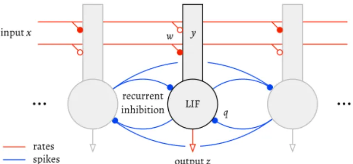
Fig. 1.Architecture of the network. Annotations indicate the feedforward inputx, leaky integrate-and-fire (LIF) somas and their firing rate z, dendritic compartments and dendritic activityy, and feedforward and recurrent pathways with weightswandq, respectively. The symbol•denotes an inhibitory synapse, ◦an excitatory one.
prevent the backpropagating action potentials from reaching the dendrites, which induces depression in dendritic synapses via spike-timing dependent plasticity.Urbanczik and Senn(2014) use probabilistic spiking neurons where the dendritic compartment tries to match the somatic potential; this results in depression when unpredicted external inputs inhibit the soma, and potenti-ation when these unpredicted inputs are excitatory instead.
Here we set out to investigate whether a variant of these somato-dendritic learning rules could discover sparse codes in natural stimuli. We found that one can adjust the somatic and dendritic transfer functions to produce a BCM-like curve where the threshold between depression and potentiation follows an in-stantaneous measure of somatic inhibition. This lets the network learn sparse codes by regulating population sparseness instead of lifetime sparseness, and does not require fast intrinsic plasticity.
2. Results
2.1. Network model
Our model is a network ofN neurons, each of which consists of a spiking, leaky integrate-and-fire (LIF) soma, and a rate-based dendritic compartment (Fig. 1). We summarise its main features here and refer the reader to the Methods section for the full details.
The dendrites have distinct receptive fields
w
and integrate feedforward input ratesxfor each stimulus, yielding a currentId:gd
=
∑
pre
xpre
w
pre→post receptive field activationy
=
max(gd,
0) dendritic activation Id=
{
y0
+
κ
y ify>
00 otherwise dendritic current
(1)
The somas integrate both the dendritic current Id and a
cur-rent Is from recurrent inhibitory synapses to drive a varying
membrane potentialu:
τ
m dudt
=
Id+
Is−
u (2)Somas emit spikes according to standard LIF dynamics with a fixed threshold, fixed reset and no refractory period. These spikes induce recurrent inhibition throughout the network via the cur-rentIs, and are also used to compute a firing ratezthat modulates
learning in both the dendritic and the somatic synapses. The network is meant to model a small patch of neural tissue where full connectivity is an acceptable approximation; hence we
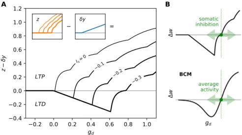
Fig. 2.The learning rule produces a BCM-like nonlinearity controlled by somatic inhibition. A: effective Hebbian nonlinearityz−δyas a function of the receptive field activationgdand somatic inhibition. Injecting a constant inhibitory currentIsinto the soma (marked on the curves) shifts the potentiation threshold to the
right. The contributions of the termsyandzare shown in insets. Bumps in the curves are a consequence of the way we compute the firing ratezand mark the occurrence of an extra spike. B: the result is a BCM-like nonlinearity controlled by somatic inhibition, whereas the BCM rule itself is controlled by average activity. Note: this figure was generated with a finer timestepdt=0.01 msto smooth the discontinuities in the curves caused by the discrete spike times..
keep the number of neurons small (N
≤
1024). With respect to the dimensionality d of our input stimuli, this translates to networks that range from undercomplete (N/
d≪
1) to slightly overcomplete (N/
d≈
1.
3).There are two fully-connected pathways: a recurrent inhib-itory pathway between the somas, and a feedforward pathway between the input and the dendrites.
The feedforward pathway targets the dendrites and contains both excitatory and inhibitory synapses. It carries rates instead of spikes; doing so allows us to employ a classical Hebbian formalism in the learning rule and discrete-time dendritic com-partments. A spike-based input and continuous-time dendrites would be more biologically plausible, but the model would also become substantially more complex; we reserve these for fu-ture work. Here we use a rectified linear activation function in the dendrites, with some modifications to account for the overall transfer properties of biological dendrites (seeMethodsfor details).
The recurrent pathway mediates all-to-all inhibition via spikes and conductance-based somatic synapses. For simplicity we do not use separate inhibitory interneurons (although that archi-tecture deviates from biology and Dale’s law,King et al.(2013) found that replacing direct inhibition with interneurons did not substantially alter the results ofZylberberg et al.(2011)). We do not model propagation delays which are de-facto fixed at one timestepdt. We allow self-inhibition for simplicity, as it has only a minor effect on receptive field formation (Fig. 5). Self-inhibition decreases the slope of the current–frequency (I–f) curve of the LIF neuron without changing its threshold (it acts like a relative refractory period and can only affect future spikes). Thus it can in theory be compensated for by parameters controlling the input gain.
The network operates as follows. We present each input pat-ternxto the dendrites and compute the dendritic activation y. This results in a constant current flowId from the dendrite to
the soma while the somas compete to respond for 100 timesteps (dt
=
0.
5 ms), producing spikes that induce time-varying in-hibitory currentsIs. Then we compute firing ratesz using boththe number of spikes and the spike latencies. Finally, we apply the feedforward and recurrent learning rules. We repeat these steps for the next input pattern, etc.
2.2. Feedforward learning rules
The weight
w
of each feedforward, dendritic synapse is up-dated according to a nonlinear Hebbian rule:w
←
w
+
µ
[x(z−
δ
y)−
yw
] (3) where xis the input rate, yis the dendritic activation,z is the somatic firing rate,µ
is the learning rate andδ
sets the potentia-tion/depression ratio. The rule can change the sign of the weights, switching between excitatory and inhibitory synapses.The core of the learning rule is the term z
−
δ
y (Fig. 2). Within that term, yis non-linear with respect to the receptive field activation gd (due to the dendritic rectification), and z isitself nonlinear with respect to y(due to the somatic response threshold, which increases with somatic inhibition). Thusz
−
δ
yis zero for sub-threshold inputs (gd
≤
0 andz=
y=
0), negativefor super-threshold inputs but weak somatic responses (gd
>
0andy
>
0, butz< δ
y), and positive for strong somatic responses (gd>
0,y>
0, andz> δ
y).This mirrors the termy(y
−⟨
y2⟩
) in the BCM rule, which is alsonon-linear with respect to the receptive field activation, inducing long-term depression (LTD) for weak responses and long-term potentiation (LTP) for strong responses. But where the BCM rule defines weak and strong responses in relation to the average activity
⟨
y2⟩
(lifetime sparseness), here we define them in terms of winning or losing the competition to respond (population sparseness).If the dendrite is active (yis large) but the soma is inhibited (z
is comparatively small), the rule induces LTD: the neuron tried to respond and lost to more active neurons. If the dendrite is active and the soma responds strongly (z
> δ
y), the rule induces LTP: the neuron is one of the winners. If the dendrite is not active (y=
0), the soma is not active either (z
=
0) and there is no synaptic change: the neuron did not participate in the competition for that particular input.The decay term
−
yw
sets a steady-state value for the weights and scales the maximum dendritic activityyas a function of the receptive field size. It is gated by dendritic activity: there is no decay when y=
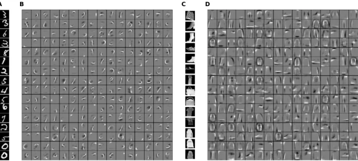
0. This ensures that the weights do not fade when the dendrite is inactive.Fig. 3. The network learns independent components from the MNIST datasets. A, B: the network learns pen-stroke shapes from the MNIST dataset. A: sample input stimuli. Black corresponds to zero and white to one. B: receptive fields (weights) of a network with 256 neurons after training on 120,000 digits (28×28 pixels) with random distortions. Middle grey corresponds to zero, lighter pixels to excitatory weights, and darker pixels to inhibitory weights. C, D: the network learns the outlines and parts of the various items of clothing in the Fashion-MNIST dataset; for instance the neuron in the top-right corner of D responds to short sleeves. All other details are the same as for A and B.
Finally, we apply a separate regularisation rule after the Heb-bian changes, taking care not to change the sign of the weight:
w
←
{
max (0
, w
−
µλ
y) ifw >
0min (0
, w
+
µλ
y) ifw <
0 (4) whereλ
determines the amount of regularisation. This does not fundamentally change the operation of the learning rule, but sim-plifies the receptive fields by suppressing the weights of weakly correlated input dimensions.In summary, the feedforward learning rule compares the den-dritic and somatic activities to estimate whether the neuron was silent, losing or winning. It then updates the weights so that inputs correlated with losing become inhibitory, inputs corre-lated with winning become excitatory, and inputs correcorre-lated with being silent are removed from the neuron’s receptive field.
2.3. Recurrent learning rule
The somatic synapses that mediate lateral inhibition are plas-tic as well. The weight q of each recurrent, somatic synapse between a pre- and a post-synaptic neuron follows a standard Hebbian rule with pre-synaptic gating:
q
←
q+
ν
(zprezpost−
β
zpreq) (5)where a constant
ν
sets the learning rate and another constantβ
controls the scale of the weights (seeMethodsfor parameter values). Gating byzpreensures that the inhibition from a winningneuron to a losing neuron decays, but the reciprocal connection does not. The asymmetry prevents a single neuron from taking over all the input features (Marshall,1995). In practice, we use a much faster learning rate for the recurrent inhibition compared to the feedforward synapses (
ν
≫
µ
); otherwise receptive fields are unstable and oscillate between selective and non-selective features.Inhibitory plasticity, as opposed to fixed inhibition, has two roles in our model. First, it ensures that neurons compete with each other only to the degree that their responses are correlated (Marshall,1995). Thus if two neurons respond to features that are only weakly correlated, they can occasionally be strongly active
at the same time without influencing each other. And second, it stabilises the feedforward learning rule just like the homeostatic threshold does in the BCM rule: it ensures that as neurons fire more they also attract more inhibition, which prevents the dis-tribution ofgdfrom escaping the LTD region of the feedforward
learning rule (Fig. 2). If the recurrent inhibitory weights were fixed, all dendrites would learn the same non-selective receptive field (Fig. 5).
2.4. Receptive fields
Our first experiment is to look at the receptive fields of the neurons after training on various types of inputs. The expecta-tion, for a sparse coding network, is that these receptive fields should correspond to selective features (rather than whole input patterns) and that the neurons should be silent most of the time. Trained on the MNIST dataset of handwritten digits (LeCun & Cortes,1998), the network learns receptive fields that respond to fragments of digits or pen strokes, as shown inFig. 3. These re-ceptive fields resemble the ones learned by sparse auto-encoders (Makhzani & Frey,2015), despite the fact that we use a different algorithm — a coincidence which can be explained if these pen-stroke shapes are indeed the independent components of MNIST digits. We also test a variant of MNIST called Fashion-MNIST (Xiao, Rasul, & Vollgraf,2017), which uses the same format but consists of small images of items of clothing like shoes and shirts. Training the network on that dataset extracts the outlines of the input stimuli and also separates some of their constituent parts.
We then train the network on two photographic datasets. The first one is the dataset used byOlshausen and Field(1997), which consists of landscapes and close-ups of natural outdoors scenes. The second one, which we refer to as the Monuments dataset, is a selection of black-and-white archive photographs from the Cornell University Digital Collections (Cornell University Library,
2008) that show monuments and cities of France. Sparse coding networks have often been applied to natural images (Butko & Triesch,2007; Olshausen & Field,1997; Savin et al.,2010; Zyl-berberg et al.,2011), from which they learn Gabor-like filters that resemble the receptive fields of simple cells in the visual cortex (van Hateren & van der Schaaf,1998). Images are typically not
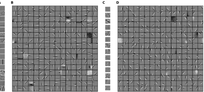
Fig. 4. The model learns oriented edge filters from pre-whitened natural images. A, B: Monuments dataset. A: sample input patches. Middle grey corresponds to zero. B: receptive fields after training on 500,000 patches (16×16 pixels) (seeMethods). In addition to the localised edge filters, the network develops a pair of non-selective ON and OFF receptive fields (uniform dark and bright patches). These encode the mean of the input, which we do not subtract. Similarly, a dozen cells learn broad oriented gradients. C, D: Olshausen & Field dataset. Receptive fields tend to be shorter and more localised than with the Monuments dataset. All other details are the same as for A and B.
Table 1
The network learns features that improve linear decoding. Mean and standard deviation of the test error on MNIST (10 runs with different random seed). For comparison we include data (†) for a MLP (28×28–300–100–10) fromLeCun, Bottou, Bengio, and Haffner(1998); other results are our own work.
Input Classifier Error (%) Raw pixels SVM (linear) 8.2 Raw pixels kNN (k=4) 3.2 Raw pixels MLP (3 layers) 2.5±0.1†
Sparse (N=256) SVM (linear) 3.3±0.2 Sparse (N=512) SVM (linear) 2.3±0.1 Sparse (N=768) SVM (linear) 2.1±0.1 Sparse (N=1024) SVM (linear) 1.9±0.1
Table 2
Sparse features also improve linear decoding on the Fashion-MNIST dataset, although less than with the standard MNIST.
Input Classifier Error (%) Raw pixels SVM (linear) 16.0 Raw pixels kNN (k=4) 14.2 Sparse (N=256) SVM (linear) 18.2±0.4 Sparse (N=512) SVM (linear) 15.5±0.2 Sparse (N=768) SVM (linear) 14.5±0.3 Sparse (N=1024) SVM (linear) 14.3±0.2
presented to the network in their raw form, but first processed either by adifference-of-Gaussiansfilter that models the transfor-mations happening in the retina, or by a whitening transform that equalises the variance across spatial frequencies (Blais, Intrator, Shouval, & Cooper,1998). Both types of pre-processing have the effect to suppress low spatial frequencies and highlight edges. For this experiment we adopt the whitening transform ofOlshausen and Field(1997).
After training on small patches drawn at random from dif-ferent image locations, the model learns oriented edge filters, in line with other sparse coding algorithms (Fig. 4). Compared to the outdoor scenes used byOlshausen and Field(1997), the Monuments dataset yields more elongated receptive fields; this is probably due to the more frequent occurrence of straight edges in scenes that contain man-made objects.
Fig. 5. Inhibitory plasticity, but not self-inhibition, is required for the learning rule to function. Receptive fields from three networks withN=64 neurons after learning from the same initial random state, but with different configurations of recurrent inhibition. In the variant with fixed inhibition, some neurons stop responding early in the learning process and still have a random receptive field; all active neurons have the same receptive field which corresponds to the average digit.
2.5. Linear decoding
The next series of experiments aims to check whether the net-work’s output is indeed a good encoding of the input. This does not necessarily follow from an analysis of the receptive fields; for instance, a network could succeed in extracting individual independent components, but still fail to encode the mixture of components present in any given input. More specifically, we would like to check whether the sparse encoding produced by the network can be linearly decoded, enabling cheap multiple readouts of cell assemblies as envisioned byFusi et al.(2016).
We first test whether sparse codes make it easier to classify MNIST digits (Table 1). Trained on the raw pixels, a linear Support Vector Machine (SVM) classifier performs poorly on MNIST, with an error rate of 8.2%. But the same linear classifier reaches a much better performance if we train it on the output of the sparse coding network instead of the raw pixels. With N
=
512 neurons, that combination outperforms the non-parametric k-Nearest Neighbours method (kNN). It also compares with a Multi-Layer Perceptron (MLP) with three layers — in that particu-lar case, the unsupervised sparse coding layer effectively replaces two hidden layers trained using backpropagation. With N
=
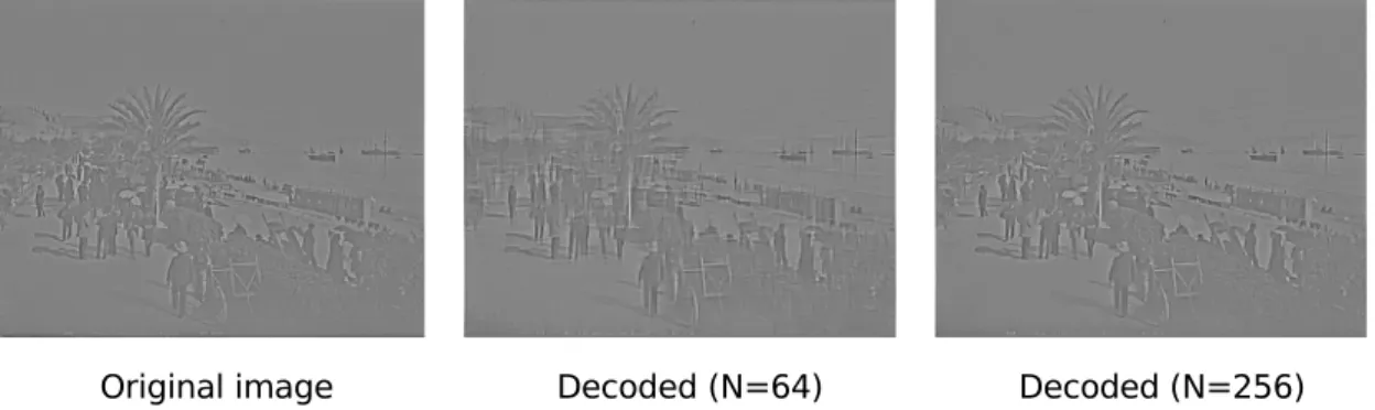
Fig. 6. Input images can be linearly decoded from the sparse output. Reconstructions from networks of 64 to 256 neurons show increasing fidelity to the original image.
higher than most non-convolutional methods with the exception of polynomial SVM (LeCun et al.,1998;Xiao et al.,2017).
We obtain broadly similar results with the Fashion-MNIST variant (Table 2): sparse coding improves linear decoding. How-ever, this dataset is more challenging than the standard MNIST digits for non-convolutional algorithms, and the improvement is consequently smaller. Ensemble learning methods as well as polynomial SVM yield a better performance (Xiao et al.,2017).
After that classification task, we turn to linear regression and attempt to reconstruct natural images from the output of the network. While Zylberberg et al. (2011) inverted the transfor-mation manually by reusing the network’s encoding weights for decoding, here we train a linear model to predict the input patch given the sparse output of the network. We did not attempt to quantify the reconstruction error: pixel-wise measures such as the peak signal-to-noise ratio are neither very informative of how much structure is preserved, nor easy to interpret when comparing different scenes, and better metrics based on struc-tural similarity are non-trivial to compute (Thung & Raveendran,
2009). Qualitatively, we find that even a small network with 64 neurons preserves the general features of the scene (Fig. 6), despite reducing the dimensionality of the data by a factor of 4.
2.6. Sparseness
The activity of the network is sparse at the end of the train-ing period, both in terms of lifetime and population sparseness (Fig. 7). Plastic recurrent inhibition rapidly enforces sparse spik-ing and maintains it at the level of a Poisson process with the same rate, or slightly higher (Fig. 8).
Lehky, Sejnowski, and Desimone(2005) make the point that lifetime and population sparseness in sensory neurons are inter-related: if the responses of the neurons are uncorrelated, then their population and lifetime sparseness must be equal, a prop-erty they call ergodicity. We find that this is indeed true of our network: for all the datasets we tested, both types of sparseness tend towards the same steady-state value as the number of neuronsNgrows sufficiently large.
However, sparseness induced by mutual inhibition is not by itself sufficient for an efficient sparseencoding of the input. With random receptive fields, decoding error increases with sparser activity.
2.7. Stability and response to perturbations
In most machine learning experiments, the input data is ran-domised so that its distribution is mostly homogeneous over time. This is not the case for embodied agents that learn continu-ously: an animal samples from small regions of the input space as it moves from one place or activity to the next. Thus an important
Fig. 7. Lifetime and population activity is sparse after training on the MNIST dataset. A: the net dendritic input (receptive field activation) has a heavy-tailed distribution (excess kurtosis: 2.82, skewness: 0.9). The two conditions (spikes/no spikes) are stacked, not overlaid. B: neurons are silent most of the time, as shown by the distribution of the number of spikes per neuron per stimulus. C: only a few spikes are emitted for each stimulus. The alternating columns in the background are 50.0 ms wide and correspond to successive MNIST patterns during a one-second period at the end of the training run.
challenge in artificial neural networks is to learn online on non-homogeneous data. Sparse coding networks with a homeostatic term make an explicit assumption that the average firing rate of each neuron is constant, and the violation of that assumption could be a factor in catastrophic forgetting. The next experiment aims to explore whether the absence of a homeostatic term in our model makes it more robust to perturbations.
InFig. 9, we first train the network on the full MNIST dataset with Gaussian noise (
σ
=
0.
2) added to the digits and clipped to[
0,
1]
. After 150000 stimuli, we remove the MNIST input and continue training on the background noise. We restore the input and train again on the full MNIST dataset for 150000 stimuli. Finally, we perform one last training round on a subset of MNIST that contains only the zeros, with all other digits removed.We find that the receptive fields retain their selectivity de-spite fading during the period when the network receives only background noise, and recover with minimal changes when the original input is restored (Fig. 10): thanks to the lack of fast IP, input deprivation does not induce catastrophic forgetting. As long
Fig. 8.Plastic recurrent inhibition enforces sparse spiking, but feedforward plasticity is required for efficient sparse coding. Treves & Rolls (TR) sparseness (top, seeMethodsfor details) and test error with a linear SVM (bottom) while training a network ofN=256 neurons on MNIST. Here we stage the learning in three phases: first with no plasticity (fixed initial weights); then activating the recurrent inhibition learning rule (soma only); and finally with both the recurrent and feedforward learning rules (soma and dendrite). The Poisson control shows the lifetime sparseness of a Poisson process with the same rate as the soma. The curves for the lifetime and population sparseness (soma) overlap almost perfectly in this figure. We increased the initial weightsw, and decreased q, so that the initial state is less sparse. SeeAnnex for a similar figure with natural images as the input.
as the distribution of the independent components remains the same, there is also no drift with continued learning (compare A and C inFig. 10). In contrast, we observed a constant shifting of the receptive fields when replicating other models such as the one byZylberberg et al.(2011).
However, the receptive fields do change rapidly when we switch from the full MNIST to zeros only: they adapt to match the new distribution of the independent components and forget the features that were specific to other digits (such as straight lines). Thus the lack of IP protects against forgetting during input deprivation but does not block continual adaptation to the input, as long as the new stimuli overlap with existing receptive fields. A small number of neurons (typically one or two) respond strongly to the noise during the period of input deprivation (bright receptive fields inFig. 10; dark lines in Figs. 9and11). Average firing rates for the other cells are low; again, this can be explained by the absence of a homeostatic term that would drive every neuron towards a target firing rate. Since the background noise does not contain any structure, these few active cells are sufficient to encode it and inhibit other neurons, protecting their receptive fields.
The transient increase in activity when the input is restored does not exceed three times the baseline: spikes remain sparse throughout, and come back to normal after 10 s (Fig. 11). Since the neurons have fixed somatic and dendritic thresholds, that increase must come from the decay of lateral inhibition or from a shift in the excitatory/inhibitory balance of the feedforward weights. In contrast, in a network with IP, homeostatic adjust-ment of the thresholds to the background noise would cause a temporary saturation of the transfer function and loss of sparse-ness when the input is restored.
3.1. Sparse coding does not require fast IP
Our findings confirm that intrinsic plasticity (IP) is not strictly required to learn sparse codes. Plastic lateral inhibition, in addi-tion to its role in decorrelating the populaaddi-tion responses, can also regulate sparseness through its effect on the nonlinear Hebbian learning rule.
The idea of enforcing population sparseness is not new — in networks where learning uses global information, one can devise a cost function with a sparseness constraint based on population activity, and minimise it to learn a suitable set of receptive fields. But this global cost information is not typically available in neural networks that use only local information for learning, in line with biology. Thus previous models (Földiák, 1990; Savin et al.,2010;Zylberberg et al.,2011) have made use of IP to enforce lifetime sparseness, as this information is readily available in each neuron. We show that this is not the only way: information about population sparsenesscanbe conveyed to local rules through mu-tual inhibition, extracted thanks to input compartmentalisation, and used to learn independent components in the same way as lifetime sparseness.
When it comes to explaining how cortical neurons might learn sparse codes, this helps to resolve a conflict of timescales. The mechanism enforcing sparseness must be faster than Hebbian learning to avoid unstability, and consequently IP is fast in models that rely on it for sparse coding. But this conflicts with what we know about IP in biological neurons: homeostatic firing rate adaptation is normally quite slow, on the order of hours or days (Chistiakova et al., 2015; Toyoizumi et al., 2014; Zenke et al.,
2017).
Enforcing sparseness via lateral inhibition instead is a bet-ter match for the data: fast adaptation of these connections is plausible through a combination of short-term facilitation and long-term potentiation of inhibitory synapses, which can occur over a timescale of seconds to minutes. Freed from the task to stabilise Hebbian learning, IP could have other computational roles on slower timescales, for instance helping to recruit pre-viously silent neurons and dendrites or adapting to ongoing slow processes like structural plasticity and developmental changes.
3.2. Compartmentalised inputs let local rules estimate population sparseness
Our learning rule has access to information about population sparseness thanks to the separation of the feedforward and re-current pathways. If these were integrated together into a single activity variable, there would be no way to distinguish weaker in-puts from stronger competition. Compartmentalised integration, with feedforward activity integrated in the dendrite and lateral inhibition integrated in the soma, disambiguates the reasons why a neuron does not fire and allows each neuron to compute a local estimate of the amount of competition with its neighbours.
Point neurons have been cost-effective approximations wher-ever simulation of thousands of neurons in real time is the aim, and moving away from that paradigm requires good reasons. Our model gives another example of the types of learning that become possible in neurons with compartmentalised inputs and may jus-tify the expense. In contrast to multi-compartmental models with detailed branching and morphology, neurons with a few input compartments are not much more expensive to simulate than point neurons, requiring only a handful of extra state variables. This makes them suitable for large-scale simulations and hard-ware implementations — the SpiNNaker and Loihi neuromorphic chips, for instance, already support compartmentalised inputs (Davies et al., 2018; Hopkins, Pineda-García, Bogdan, & Furber,
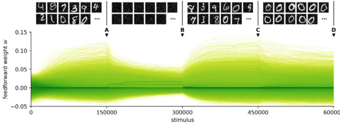
Fig. 9. Weights converge smoothly to a steady state after perturbations in the input.Top: sample training stimuli for each of the four training periods.Bottom: density plot of the trajectories of the 112896 feedforward weightswduring training (N=144). The colour mapping is logarithmic to account for the high density of zero weights. The letters A, B, C and D mark the times when snapshots of the receptive fields were taken (Fig. 10).
Fig. 10. Snapshots of the receptive fields at the times marked inFig. 9. A: receptive fields at the end of the initial training period. B: receptive fields fade during input deprivation, but do not drift. C: they recover with minimal changes after the original input is restored. D: reorganisation occurs after further training with zeros only.
3.3. Sparse coding via population sparseness is robust to input de-privation
Without fast IP, the network can be made more robust to tem-porary input deprivation. If the input is replaced by background noise, lateral inhibition will adjust in seconds, just as fast IP would rapidly adjust the firing threshold. But the important information is in the receptive fields of the dendrites, and in our model these do not adapt rapidly when the neurons are exposed to noise.
Dendrites respond weakly to noise because noise, lacking structure, tends to activate their excitatory and inhibitory recep-tive fields equally. At the population level, a couple of neurons will eventually develop broad excitatory receptive fields and start responding to the noise. But because there is no structure in noise to support a division of labour between output neurons, the first few responders will be able to inhibit all the others. This keeps the overall activity low and protects most receptive fields from change: the feedforward learning rule (Eq.(3)) is gated by post-synaptic activity and weights will not change fast if the dendrite is weakly active and the soma is inhibited.
In contrast, in models with IP, input deprivation causes a rapid adjustment of the spiking or plasticity thresholds to maintain the same average firing rate. Consequently the rate of feedforward synaptic changes stays high, and receptive fields are lost to the background noise.
But replacing intrinsic plasticity with synaptic plasticity is still not enough to cope with other types of changes, such as those that an animal or robot would encounter as it switches
between tasks and environments: the network remains suscep-tible to rapid and extensive reorganisation when novel inputs overlap the existing receptive fields, or when the distribution of the independent components changes. On the one hand, that kind of adaptability is desirable as natural environments are not static and the quick acquisition of novel stimuli can be critical for survival. On the other hand, it should disturb existing receptive fields as little as possible so as not to erase previous experiences and all the associations that build upon them.
Although increasing sparseness and careful tuning of learning rates could help, it is likely that solving that stability-plasticity dilemma will require ad-hoc gating mechanisms. Some candi-dates are the conditional consolidation of synaptic changes ( Re-dondo & Morris, 2011), neuromodulation and attention ( Has-selmo, 1995; Krichmar, 2008), or a mechanism based on top-down prediction errors like the Adaptive Resonance Theory (Grossberg,1980).
3.4. Sparse activity does not imply sparse coding
We observe a dissociation between measures of sparseness and measures of decoding accuracy: high sparseness is achieved almost immediately via the potentiation of lateral inhibitory weights, while high decoding accuracy requires adequate re-ceptive fields learned by the feedforward plasticity rule. In fact decoding accuracy in a network with random receptive fields decreases with sparseness. ConverselyZylberberg and DeWeese
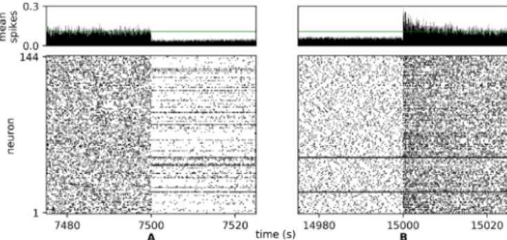
Fig. 11. The network is robust to input deprivation.Top:mean number of spikes per neuron per stimulus; the green line marks the average value before mark A.
Bottom:raster plot of the output spikes. Following input deprivation (mark A), firing patterns return to normal within 20 s after the input is restored (mark B), except for the neurons that responded strongly to the noise (these take somewhat longer).
(2013) observed decreasing sparseness as a result of receptive field formation in their sparse coding network.
Thus there is more to sparse coding than just sparse activity. Sparseness is a constraint for learning, not by itself a guarantee of an efficient encoding: sparse coding requires receptive fields that match the independent components of the input, so that the same amount of information can be transmitted with fewer spikes and fewer active units.
Lehky et al.(2005) caution that high measures of sparseness can be obtained trivially via non-linear, information-discarding transforms. For instance the average lifetime sparseness could be increased simply by raising the thresholds of the neurons, without learning selective receptive fields; but this would also decrease the information transmitted about the input. They argue that statistical measures of sparseness are not a sufficient opti-mality criterion for explaining the architecture of nervous sys-tems, and that information transmission and other ecologically-relevant aspects must also be considered.
Here we evaluate linear decodability, in the light of the hy-pothesis that the computational cost of decoding is a major bio-logical constraint together with coding density and metabolic ef-ficiency, and that linear decoding requires fewer synapses. Other criteria could be also be examined, such as whether output cor-relations are still relevant for decoding (Latham,2005), or robust-ness to noise and to the loss of coding units.
3.5. Comparison with similar models
Our model is far from being the first to learn features similar to the ones observed in V1 cells, but it differs from previous models in several ways. The learning rule used by Olshausen & Field ( Ol-shausen & Field,1997) minimises the output reconstruction error, as do sparse auto-encoders (Makhzani & Frey,2015), whereas our model does not need or compute that information. This reduces the number of steps required for learning, and as a model of sparse coding in the brain it requires neither multiple layers nor a biological mechanism for the backpropagation of error.Földiák
(1990),Zylberberg et al.(2011) andKing et al.(2013), and models based on the standard BCM rule rely on homeostatic threshold adaptation, while Savin et al. (2010) also use IP to adjust the transfer function of the neuron. Our model uses fixed thresholds instead, both in the dendrite and the soma, relying on population rather than lifetime sparseness as discussed before.
The term x(z
−
δ
y) at the core of the feedforward learning rule is reminiscent of the error-correcting Delta rule (Sutton & Barto,1981;Widrow & Hoff,1960), and it can be seen as a rate-based relative of the rules used inKörding and König(2000) andUrbanczik and Senn(2014).
the mismatch between the somatic activity,z, and its prediction by the dendrite,
ϕ
(y), so that the dendrite learns to move the somatic membrane potential towards the equilibrium potential of predictable somatic inputs. After learning, that dendritic predic-tion is mostly correct,z≈
ϕ
(y) and the predicted somatic inputs have no effect.In contrast, the goal of our learning rule is not to achieve a perfect prediction of the somatic inputs by the dendrite, but to exploit the mismatch betweenzandyso that it creates a BCM-like curve modulated by inhibition. Thus the steady state does not occur atz
≈
δ
y. Starting from the learning rule: dw
=
x(z−
δ
y)−
yw
, let us treatx,w
,zandyas correlated random variables. Then, for⟨
dw
⟩ =
0, we have⟨
x(z−
δ
y)⟩ = ⟨
yw
⟩
. Substitutingw
with a constantw
∞, we get the following non-trivial fixed point:w
∞=
⟨
x(z−
δ
y)⟩
⟨
y⟩
In other words, the fixed point over a certain set of inputs is when each weight equals the mean of the loser/winner function
z
−
δ
y(Fig. 2) times the input, normalised by the mean dendritic activity. This yields receptive fields which are inhibitory for input dimensions associated with losing the competition (z< δ
y) and excitatory for those associated with winning (z> δ
y). If there was no mismatch betweenzandδ
yin the steady state, the receptive fields would be blank (w
∞=
0).The model byKörding and König(2000) is perhaps the closest to our work. In their network, lateral inhibition decides whether a neuron is losing or winning the competition by blocking the backpropagating action potentials, switching the sign of plasticity in the dendrite. However, it does so without blocking the spikes that travel down the axon, whereas lateral inhibition in our model suppresses both the internal teaching signal and the output of the neurons. The distinction could have its relevance in multi-layer networks; but it is likely that both architectures can perform sparse coding with the right dendritic learning rule — something
that Körding and König (2000) did not explore, as they used
simple stimuli such as moving bars which do not contain multiple independent components.
3.6. Biological interpretation
Our model is only loosely based on biology: at its core, it is mainly a computational exploration of compartmentalised input integration in the context of sparse coding, and whether bio-logical neurons make use of similar principles remains an open question. But it does suggest phenomenological interpretations for a number of experimental facts.
In terms of architecture, there are multiple inhibitory path-ways in the cortex (Kubota, Karube, Nomura, & Kawaguchi,2016), and some of these pathways target dendrites or somas specif-ically as they do in our model; for instance the fast-spiking, parvalbumin-positive basket cells mediate lateral inhibition pref-erentially via synapses close to the soma. There are, however, many other pathways, including recurrent inhibitory pathways targeting dendrites, that our model does not explain.
As for synaptic plasticity, let us rearrange the terms of the feedforward learning rule (Eq.(3)) and annotate it to match the terminology used in neuroscience:
∆
w
∝
homosynaptic LTP
xz−
δ
xy
homosynaptic LTD−
heterosynaptic LTD
yw
(6)put and may be linked to competition for metabolic resources between synapses. While developing our model we tested a variant (
−
zw
) for this term which depended onz instead ofy. This yielded inferior decoding performance but similar receptive fields, therefore we do not want to make a strong claim of the dendritic vs. somatic dependence of heterosynaptic LTD.Less obvious is the notion that correlated dendritic activity should induce homosynaptic LTD (
−
xy): We know, on the con-trary, that dendritic spikes can sometimes induce LTP on their own (Remy & Spruston,2007;Sjostrom, Rancz, Roth, & Hausser,2008). But we also know that NMDA receptor activation can induce LTD or act as a negative feedback on potentiation (Bear & Malenka,1994;Sjostrom et al.,2008), which is compatible with our learning rule.
In terms of learning paradigms, our model makes hypothe-ses that diverge from the classical framework of spike timing-dependent plasticity (Bi & Poo,2001), where low firing rates tend to induce homosynaptic LTD and high firing rates tend to induce homosynaptic LTP in a way that is compatible with the standard BCM rule (Izhikevich & Desai,2003).
In contrast, our model assumes that low post-synaptic rates cause homosynaptic LTD of dendritic synapses only when they are due to strong recurrent inhibition, and not to a weak feed-forward input. Conversely, it assumes that recurrent inhibition can switch the sign of plasticity at dendritic synapses and turn LTP into LTD, an idea that has been suggested in computational models (Körding & König,2000;Wilmes, Sprekeler, & Schreiber,
2016) but requires further experimental validation.
Other aspects of biological neurons, however, are more diffi-cult to reconcile. For instance, our model relies on lateral inhi-bition shifting the response curve of the somas to the right — a phenomenon known as subtractive inhibition, in contrast with divisive inhibition which modulates the response slope without changing its threshold. But in pyramidal neurons somatic inhibi-tion is normally divisive rather than subtractive: it is dendritic inhibition that has a subtractive effect (Wilson, Runyan, Wang, & Sur,2012). It may be that the mechanisms we distribute over a somatic and a dendritic compartment, occur within dendrites
in biology, possibly involving compartmentalisation between the dendritic shaft and the spines, or between different dendritic variables like voltage and calcium.
More generally, interpreting our learning rule calls for fur-ther electrophysiological investigations of how different path-ways contribute to synaptic plasticity — looking not just at pairs or triplets of pre and post spikes, but also at coincident dendritic activity and inhibitory modulation.
3.7. Relevance for machine learning
Most of the recent advances in machine learning have relied on supervised learning, and there have been efforts to make supervised learning algorithms like error backpropagation work with spiking neurons as well (Sacramento, Costa, Bengio, & Senn,
2018;Zenke & Ganguli,2018). But there is also a notion that un-supervised learning will play an increasing role in future learning
4. Models & methods
4.1. Somatic compartments and somatic synapses
The somatic compartments are standard LIF neurons. The membrane potentialufollows the following equation:
τ
m dudt
=
Id+
Is−
u (7)whereIdand Is are the currents from the dendrite and somatic
synapses, respectively.
We use a fixed spiking threshold
θ
and after-spike resetρ
without a refractory period:u
←
ρ
ifu≥
θ
(8)We compute a firing ratezthat takes into account the number of spikes and also their latency relative to the stimulus onsett0,
with the aim of producing a smooth measure that is sensitive to small changes in activity even in the case of a single spike. First we define a trace
ζ
that increases after each spike and decays exponentially:ζ
←
ζ
+
1 ifu≥
θ
τ
ζdζ
dt= −
ζ
(9)
Then we normalise so that the area under the curve is the number of spikes, and integrate over the stimulus window:
z
=
∫
t0+50mst=t0
ζ
τ
ζdt (10)Thus a spike that occurs towards the end of the window con-tributes less to the total than a spike that occurs early. This also approximates the effect of input eligibility traces in more detailed models.
Somatic inhibition comes from lumped, conductance-based synapses where the fractiongsof active conductance and somatic
currentIsevolve as follows for each neuron post: gs
←
gs+
qpre→post on spike from neuron preτ
s dgsdt
= −
gs Is= −
gsu(11)
The initial weightsqare drawn from an exponential distribu-tion (mean
=
0.
01).Before each new stimulus we reset the continuous-time vari-ables of the model, as inZylberberg et al.(2011):
u
←
ρ
ζ
←
0gs
←
0(12)
That reset does not seem to be critical for our findings, but we did not explore the issue further.
Dendrites are rate- and current-based. The net dendritic input
gdand dendritic activationyfor each neuron post are as follows:
gd
=
∑
pre
xpre
w
pre→posty
=
max(gd,
0)(13)
The initial weights
w
are drawn from a normal distribution (std=
0.
01).The currentId from the dendrite to the soma is a nonlinear
function of the dendritic activation:
Id
=
{
y0
+
κ
y ify>
00 otherwise (14)
Here the goal is to reproduce the active properties of biological dendrites. Above a certain input threshold, regenerative activa-tion of the NMDA receptors causes dendritic spikes. These lead to a sharp increase in membrane potential followed by a plateau where stronger inputs cause no further increase in voltage ( Milo-jkovic, Radojicic, & Antic,2005;Oikonomou, Short, Rich, & Antic,
2012). We model this with a step function and the offset y0.
However, stronger inputs do increase the duration, and reduce the rise time of the plateau, producing more somatic spikes. We model this with the linear term
κ
y. In practice we adjusty0 to cancel out the somatic rheobase, so that suprathreshold
dendritic activation elicits at least one spike in the absence of somatic inhibition. Dendrites start responding whengd
>
0. Wefind that the actual threshold is not critical for our findings as long as all dendrites respond to some inputs at the start of the simulation. A small positive value would better reproduce the data inMilojkovic et al.(2005) andOikonomou et al.(2012).
The coupling between the soma and the dendrite is one-way: somatic potentials have no effect on dendritic activity in our model. This ignores the effect of backpropagating action potentials on dendritic voltage, but it does match the data on somatic inhibition, which has almost no impact on the generation of dendritic spikes (Jadi, Polsky, Schiller, & Mel,2012; Rhodes,
2006).
4.3. Measure of sparseness
InFig. 8we use the same measure of sparseness asZylberberg and DeWeese(2013), called TR sparseness after Treves & Rolls and related to the coefficient of variation. It is computed as follows: Str(X)
=
(
1−
⟨
X⟩
2⟨
X2⟩
) (
1−
1 n)
−1wherenis the length ofX.
For lifetime sparseness, X is a vector of 1000 observations from the same neuron over time, and we then averageStracross
all neurons in the population. For population sparseness, it is a vector of observations from allNneurons across the population at a particular instant, andStris averaged over 1000 stimuli. Somatic
sparseness uses the number of spikes (one could use the output ratez, but the number of spikes is easier to compare to a Poisson control) while dendritic sparseness uses the dendritic activityy.
In our case the Gini index gives qualitatively similar results to TR sparseness, and could be used interchangeably. Both are more stable over time than excess kurtosis, as noted byHurley and Rickard(2009).
Model parameters used for all experiments in this paper. Soma and somatic synapses Dendrites
θ=1.0 y0=1.0 ρ=0.0 κ=0.5 τm=10.0 ms δ=0.5 τζ=50.0 ms λ=0.01 τs=5.0 ms µ=4×10⁻⁴ ν=1×10⁻¹ β=N/250 4.4. Parameters
Table 3summarises the parameters for the neuron model. All simulations are performed with a timestepdt
=
0.
5 ms and 100 steps per stimulus, except forFig. 2which uses a finer timestep.4.5. Receptive fields
Throughout this paper we use the weights of the neurons as a proxy for their actual receptive fields. Showing all the weights of the network on the same image requires that we normalise each receptive field separately, because neurons that respond to narrow features have larger absolute weights than those that respond to broad ones. Nonetheless, we make sure that zero weights appear as the same middle grey for all neurons, allowing quick identification of ON (brighter) and OFF (darker) areas. Thus we normalise the receptive field Wi
=
[
w
1→i· · ·
w
d→i]
of each neuronias follows when generating the figures:
Wi′
=
1+
aiWi 2 (15) where ai=
(
max1≤j≤d|
w
j→i|
)
−1and d is the number of input dimensions.
4.6. MNIST
We use both the standard MNIST dataset (LeCun & Cortes,
1998) and the Fashion-MNIST variant (Xiao et al., 2017), each with 60,000 training samples and 10,000 test samples. We map the full range of the data to the interval
[
0,
1]
. When training the sparse coding network, we shuffle the patterns and distort them with random shears and translations, as done inLeCun et al.(1998). The purpose of these distortions is to increase the number of distinct training samples, and also to remove the correlations introduced by the centring of the patterns. We do this by applying the following affine transformation with the origin at the centre of the pattern: M
=
[
1 A 1 T1 A2 1 T2 0 0 1]
where eachAiis a random variable drawn fromN(
σ
=
0.
1), andeachTi is a random variable drawn fromN(
σ
=
2.
0). Distorteddigits produce more localised receptive fields than the centred patterns, which in turn improves the performance of classifiers trained on the output of the network. When training and testing the classifiers themselves, we freeze the weights of the sparse coding network and we use the plain stimuli without distortions.
In Table 1 we use the following classifiers from
scikit-learn
(Pedregosa et al.,2011) version 0.19.1:SVM:
LinearSVC(C=1.0, class_weight=None,
dual=Fal-se, fit_intercept=True, intercept_scaling=1,
loss=
squared_hinge,
max_iter=1000,
multi_
class=ovr
,penalty=l2, random_state=2136146589,
tol=0.0001, verbose=0)
200,000 pixels, preprocessed using the same whitening trans-form asOlshausen and Field(1997), and then normalised to unit variance. No further normalisation was applied to the individual patches used for training; in particular, the patch mean was not subtracted from the input. Note that in contrast to MNIST the natural image stimuli contain both positive and negative values. We interpret these as ON and OFF channels from the retina; while it would be more realistic to split the ON and OFF values into separate, non-negative channels, we did not attempt this here.
For the reconstruction experiment, the input image was tiled into overlapping patches with a width of 16 pixels and a stride of 8 pixels. Each input patch was run through a sparse coding network pre-trained on the Monuments dataset. The sparse out-put was then fed as the inout-put to a linear model trained with ridge regression to reconstruct the original patches. Finally, the predicted patches were placed at their original locations and averaged to account for the stride overlap.
Declaration of competing interest
The authors declare that they have no known competing finan-cial interests or personal relationships that could have appeared to influence the work reported in this paper.
Acknowledgements
DD and VVH were funded by the GRK 1589/1 and 1589/2 Sen-sory Computation in Neural Systems of the Deutsche Forschungs-gemeinschaft (DFG).
DD and VVH were funded by EU FP 7 Grant 609465 (EARS). DD and MS were funded from EU FP 7 Grant 604102 and H2020 Grants 720270, 785907 and 945539 (Human Brain Project SGA1, SGA2 and SGA3).
Annex
SeeFig. 12.
References
Barlow, H. B. (1987). Cerebral cortex as model builder. In L. Vaina (Ed.),Matters of intelligence. Dordrecht: Springer, http://dx.doi.org/10.1007/978-94-009-3833-5_18.
Bear, M. F., & Malenka, R. C. (1994). Synaptic plasticity: LTP and LTD.Current Opinion in Neurobiology, (3), http://dx.doi.org/10.1016/0959-4388(94)90101-5.
Bell, A. J., & Sejnowski, T. J. (1995). An information-maximization approach to blind separation and blind deconvolution.Neural Computation, (6),http: //dx.doi.org/10.1016/0165-1684(91)90081-S.
Bi, G.-q., & Poo, M.-m. (2001). Synaptic modification by correlated activity: Hebb’s postulate revisited.Annual Review of Neuroscience, (1),http://dx.doi. org/10.1146/annurev.neuro.24.1.139.
Bienenstock, E. L., Cooper, L. N., & Munro, P. W. (1982). Theory for the development of neuron selectivity: orientation specificity and binocular interaction in visual cortex.Journal of Neuroscience, (1),http://dx.doi.org/10. 1523/JNEUROSCI.02-01-00032.1982.
Fig. 12. Sparseness follows a similar timecourse with natural images. Same as the top part ofFig. 8, but this time training on the Monuments dataset of natural images instead of MNIST. In this case we did not compute a reconstruction error.
Blais, B. S., Intrator, N., Shouval, H. Z., & Cooper, L. N. (1998). Receptive field formation in natural scene environments: Comparison of single-cell learning rules.Neural Computation, (7),http://dx.doi.org/10.1088/0954-898X/7/3/003. Brito, C. S. N., & Gerstner, W. (2016). Nonlinear hebbian learning as a unifying principle in receptive field formation.PLoS Computational Biology, (9),http: //dx.doi.org/10.1371/journal.pcbi.1005070.t001.
Butko, N. J., & Triesch, J. (2007). Learning sensory representations with intrinsic plasticity. Neurocomputing, (7–9), http://dx.doi.org/10.1016/j.neucom.2006. 11.006.
Buzsáki, G. (2010). Neural syntax: Cell assemblies, synapsembles, and readers. Neuron, (3),http://dx.doi.org/10.1016/j.neuron.2010.09.023.
Castro-Alamancos, M. A., Donoghue, J. P., & Connors, B. W. (1995). Different forms of synaptic plasticity in somatosensory and motor areas of the neocortex.Journal of Neuroscience, (7),http://dx.doi.org/10.1523/JNEUROSCI. 15-07-05324.1995.
Chistiakova, M., Bannon, N. M., Chen, J.-Y., Bazhenov, M., & Volgushev, M. (2015). Homeostatic role of heterosynaptic plasticity: models and exper-iments. Frontiers in Computational Neuroscience, http://dx.doi.org/10.3389/ fncom.2015.00089.
Cornell University Library (2008). Andrew Dickson white architectural photographs collection — France. Cited 28 November 2018. Avail-able from: https://www.flickr.com/photos/cornelluniversitylibrary/albums/ 72157617483156826.
Davies, M., Srinivasa, N., Lin, T.-H., Chinya, G., Cao, Y., et al. (2018). Loihi: A neuromorphic manycore processor with on-chip learning. IEEE Micro, (1), http://dx.doi.org/10.1109/MM.2018.112130359.
Diaconis, P., & Freedman, D. (1984). Asymptotics of graphical projection pursuit. The Annals of Statistics,12(3), 793–815, Available from:http://www.jstor.org/ stable/2240961.
Falconbridge, M. S., Stamps, R. L., & Badcock, D. R. (2006). A simple hebbian/anti-hebbian network learns the sparse, independent compo-nents of natural images.Neural Computation, (2),http://dx.doi.org/10.1162/ 089976606775093891.
Ferré, P., Mamalet, F., & Thorpe, S. J. (2018). Unsupervised feature learning with winner-takes-all based STDP. Frontiers in Computational Neuroscience, http://dx.doi.org/10.3389/fncom.2018.00024.
Földiák, P. (1990). Forming sparse representations by local anti-hebbian learning. Biological Cybernetics,http://dx.doi.org/10.1007/BF02331346.
Fusi, S., Miller, E. K., & Rigotti, M. (2016). Why neurons mix: high dimensionality for higher cognition. Current Opinion in Neurobiology, http://dx.doi.org/10. 1016/j.conb.2016.01.010.
Grossberg, S. (1980). How does a brain build a cognitive code?Psychological Review, (1),http://dx.doi.org/10.1037/0033-295X.87.1.1.
Hafner, V. V., Fend, M., König, P., & Körding, K. P. (2004). Predicting properties of the rat somatosensory system by sparse coding.Neural Information Processing Letters and Reviews,4(1), 11–18, Available from: http://bsrc.kaist.ac.kr/nip-lr/V04N01/V04N01P2-11-18.pdf.
Hasselmo, M. E. (1995). Neuromodulation and cortical function: modeling the physiological basis of behavior.Behavioural Brain Research, (1),http://dx.doi. org/10.1016/0166-4328(94)00113-T.
Hawkins, J., & Ahmad, S. (2016). Why neurons have thousands of synapses, a theory of sequence memory in neocortex. Frontiers in Neural Circuits, http://dx.doi.org/10.3389/fncir.2016.00023.
Hebb, D. O. (1949).The organization of behavior: A neuropsychological theory. John Wiley & Sons, Inc., ISBN: 9781410612403.
Hopkins, M., Pineda-García, G., Bogdan, P. A., & Furber, S. B. (2018). Spiking neural networks for computer vision. Interface Focus, (4),http://dx.doi.org/ 10.1098/rsfs.2018.0007.