U
NIVERSIT
AT
¨
A
UGSBURG
A Comparative Study of Sequential Feature
Selection Methods for Support Vector
Machine
Jonghwa Kim
Report 2007-10 October 2007
I
NSTITUT F
UR
¨
I
NFORMATIK
D–86135 Augsburg, Germany
http://www.Informatik.Uni-Augsburg.DE — all rights reserved —
1
A Comparative Study of Sequential Feature
Selection Methods for Support Vector Machine
Jonghwa Kim
Institut f¨ur Informatik, Universit¨at Augsburg [email protected]
Abstract—In this paper we investigate existing
fea-ture selection algorithms combined with support vector machine (SBS). Two ranking-based algorithms, recursive feature elimination (RFE) and incremental regularized risk minimization (IRRM), and greedy sequential backward search (SBS) are tested by using biosignal dataset which contains 35 features per sample and a total of 25 samples labeled by four emotion classes. The performance of the selection algorithms are compared by considering recognition rates obtained by the leave-one-out validation.
I. INTRODUCTION
N
OWDAYS in many pattern classification problems it is not uncommon that we are confronted with a very high dimensional variable space, with hundreds to tens of thousands of attributes or features. In this case, not only the “curse of dimensionality” caused by a very high ratio of number of features to number of data samples is problematic but also the irrelevant fea-tures in the feature set that undermine the performance of a given learning algorithm. The purpose of feature selection is to eliminate irrelevant and noisy features in the original feature set and to find a new feature subset which can improve computational and functional performance of a given classifier. Since most supervised learning algorithms such as support vector machine (SVM) do not offer the opportunity for automatically filtering the irrelevant and redundant features, feature selection/reduction as preprocessing plays an important role in pattern classification system. A well selected feature subset does help gain a deeper insight about the concept to be learned and generalize the performance of classifier with reduced computational cost.There are a number of papers in this special issue. We refer to [1] and [2] for a comprehensive survey. In general, one can approach to feature selection through one of two ways: given a number of selected features m n, where n is number of features, find the m features that give the smallest expected generalization error, or given a maximum allowable generalization error γ, find the smallest number m of features. Note that
choices ofmin former case can usually be parameterized as choices of γ in latter case [3]. Based on the nature of algorithms, most methods for feature selection can be categorized to two types, i.e. the filter method and wrapper method. For filter approach one performs a fea-ture selection with regard to some predefined relevance measure before applying a given induction algorithm, accordingly such methods evaluate a feature based on its marginal contribution to the class discrimination without considering its interaction with other features. Wrapper methods, on the other hand, use the learning algorithm, which is used for classification, as induction method for evaluation criterion. Hence designing of a wrapper method depends on the classifier.
In this paper, we present a comparative analysis of different wrapper feature selection methods which are adapted particularly to the SVM classifier. For validation of the selected features, we used the feature set that are extracted from biosignal dataset in our previous work on emotion recognition [4]. The performance of selec-tion methods were compared with sequential backward selection (SBS) method.
II. FEATURESELECTION METHODS FORSVM
A. Support Vector Machine
The support vector machine is a binary classifier algorithm that looks for an optimal hyperplane (Fig. 1) as a decision function in a high-dimensional space [5], [6].
In supervised classification task we have a training dataset{xk, yk} ∈Rn×{−1,1}, wherexkare the
train-ing samples andykthe class labels. Before of computing
a decision function one needs to make a mappingxinto a high dimensional space using a function Φ. Different mappingsx→Φ(x)∈ Hconstruct different SVMs. The following function describes an equation of separating the hyperplane:
f(x) =w,Φ(x)+b=
k
α0kykKxk,x+b (1)
whereK is a kernel function defined as an inner product in H. Thus, the goal of the SVM is to maximize the distance to the closest image Φ(xk) from the training samples. The optimization problem, where misclassified examples from the SVM classifier will be quadratically penalized, can be written as,
min w,ξ 1 2w2+C m k=1 ξk2 (2)
under the constraint∀k, ykf(xk)≥1−ξk. In Eq. 2,w
is inverse to the margin size and · is the 2-norm and the regularization constant C > 0 determines the trade-off between the empirical error and the complexity term. The solution of Eq. 2 can be obtained by using the Lagrangian multipliers: w= m k=1 α∗kykΦ(xk) (3) where α∗k is the solution of the following quadratic
optimization problem: maxα W(α) = m k=1 αk−12 m k,l αkαlykyl K(xk,xl)+1 Cδk,l (4) subject to mk=1ykαk = 0 and ∀k, αk ≥ 0, where δk,l
is the Kronecker delta andK(xk,xl) =Φ(xk),Φ(xl)
is the Gram matrix of the training samples.
B. Ranking algorithms for SVM
In ranking algorithms for feature selection in liter-ature, different criteria Ct and their combinations are
used such as bounds which operate with weight vector
w2, radius/margin bound R2w2, R2W2 or span estimate. Also different variable space search algorithms are used like a greedy algorithm or gradient descent. Furthermore, for each criterion, two approaches sim-ilarly to neural network based variable selection are proposed in the work [7], zero-order method and first-order method. Zero-first-order method uses the criterion Ct
directly for variable ranking and identifies the variable
that produces the smallest value of Ct when removed.
Hence, the ranking criterionRc(i) =Ct(i), whereCt(i) is
the criterion value when variableihas been removed. In the latter method, derivatives of the criterion with regard to each variable are used. So one estimates the influence of the variable on the criterion which is calculated as an absolute value of the derivative. Ranking criterion is then Rc(i) =|∇Ct(i)|.
1) SVM-Recursive Feature Elimination Algorithm:
The most common feature selection algorithm for SVM is the recursive feature elimination (RFE) algorithm. This realizes an idea of sequential backward selection and is based on finding a subset, which supplies the best result. RFE begins with all the features and removes one feature at a time, which most completes an input dataset. As notedα∗k is the solution of Eq. 4 and α∗k(i) denotes the
corresponding solution, when i-th feature is removed. Ranking criterion for a given variablei is then,
w2− w(i)2=1 2 k,j α∗kα∗jykyjK(xk,xj) (5) − k,j α∗k(i)α∗j(i)ykyjK(i)(xk,xj)
whereK(i) is the Gram matrix of the training data when variable i is removed. In this case each feature obtains its own ranking. For a given dataset with the size of d, the goal is to remove r features (r < d) based on the ranking value for which the result of Eq. 5 becomes minimal. The elimination procedure is repeated until the number of features has been reached. α∗k(i) is supposed
to be equal toα∗k, even if a variable has been removed.
Note that this algorithm is identical to the zero-order method withw2 criterion, since the first sum in Eq. 5 is constant during the evaluation of Rc(i). Although the RFE algorithm provides a fast selection, it can lead to suboptimal solutions because it uses a greedy strategy to perform backward elimination.
2) SVM-IRRM Algorithm: Incremental regularized
risk minimization (IRRM) algorithm proposed in [8] is based on the SVM-RFE approach. The basic idea of the algorithm is as follows: one calculates a ranking value for each feature and than divides all these features with regard to their ranking in sets S andR. Hence, given d features, the setS constrainsm features which are used for the classifier and the setRconsists ofd−mfeatures which are the removed features. Since there might be features in R which are relevant to classification, one combines the features of set S with some features of set R in order to improve classification accuracy with reduced regularized risk. Table I shows the algorithm and we refer to [8] for more detailed description of algorithm.
3
IRRM algorithm perform RFE
S = set of selected feature
R = set of removed features (queue) t= 0 repeat Sold=S repeat Rold reg=Rreg
compute Rreg for feature in S
if Roldreg< Rreg
restore old S
C=η highest ranked features from R
S←S∪C R←R−C
remove η features from S according to (5)
put removed features at the end of queue R
until convergence
resort queue R by means of RFE t←t+ 1
until S==Sold AND t >1
return best solution S∗
TABLE I IRRM ALGORITHM
For each feature in new set S obtained by combiningS with the features in R, the regularized risk should be calculated,
Rreg[f] =Remp[f] +1
2w2 (6)
where Remp denotes the empirical risk (training error), i.e. Remp[f] = 1 n n i=1 l(xi, yi, f(xi)) (7) The regularized risk in Eq. 6 is an upper bound on the expected generalization error (risk) over all possible patterns drawn from the unknown distribution P(x, y), i.e.,
R[f] =
x,yl(x, y, f(x))dP(x, y) (8)
If the regularized risk does not change significantly any more, one assumes that the algorithm is converged. Then one resorts the queue by means of RFE and restarts the whole algorithm.
3) Gradient methods: Main idea of gradient method
is to estimate the sensitivity of a bound with respect to a variable. For example, one introduces a scaling factor and then computes the gradient of a criterion with respect to the scaling factor υ. The computation of gradient can be performed by componentwise multiplication on the input variables and the kernelk(x,x)becomesk(υ·x, υ·
x). As a result, for a Gaussian Kernel i.e., k(υ·x, υ·
x) =e−|υ·x−υ·x |2
2σ2 , one obtains following derivatives,
∂k ∂υi =− 1 σ2(υixi−υix i)2k(x,x) (9) =− 1 σ2(xi−x i)2k(x,x)
assuming that υi = 1. The ranking term for a given criterionCt becomes then,
Rc(i) =∂Ct(α, b)
∂υi
(10)
whereCtis eitherw2,R2w2orpα∗pSp2and depends
on the solution of Eq. 4. and the bias b. Both criterions are based on radius/margin bound and are nearly. Four ranking terms obtained by using the results of [9][10] are as following:
• weight vector gradient: Rc(i) = i,j α∗kα∗jykyj∂k(υ·xk, υ·xj) ∂υi • radius/margin gradient: Rc(i) =w2 k,j (βkβj−βkδk,j)∂k(υ·xk, υ·xj) ∂υi + R2 k,j α∗kα∗jykyj∂k(υ·xk, υ·xj) ∂υi
where R2 is the optimal objective function of the following problem: max β k βkk(υ·xk, υ·xk)− k,j βkβjk(υ·xk, υ·xj) where kβk andβk≥0, ∀k.
• span estimate gradient: Rc(i) = l p=1 2−H−1∂H ∂υiα ∗ ppS 2 p+ α∗pSp4 ˜ KSV−1∂ ˜ KSV ∂υi ˜ KSV−1 pp whereH is the matrix
H= KY Y YT 0 andKkjY =ykyjk(υ·xk, υ·xj)
III. EXPERIMENT
In order to investigate the performance of the feature selection methods described above, we used biosignal dataset from our previous work on emotion recognition [4]. The feature set contains 25 samples and each sample consists of 35 features. It is labeled by four emotional classes, i.e., joy, anger, sad, and pleasure. The original biosignal dataset was recorded by using four channel biosensors, electromyogram (EMG), electrocardiogram (ECG), skin conductivity (SC), and respiration change (RSP) while the subject was listening to music songs which the subject carefully handpicked with regard to the four target emotions.
Each of the four emotions represents four quadrants of 2-D emotion model, respectively, which is spanned by two axes, arousal and valence [11]. For supporting more detailed insight into characteristics of the selection meth-ods, we performed two cases of binary classification, instead of a direct four-class classification. For arousal classification, the samples of joy and anger were labeled as high arousal, and sad and pleasure as low arousal. For valence classification, the samples of anger and sad were labeled as negative valence, and joy and pleasure as positive valence.
We tested three feature selection methods, SVM-RFE, SVM-IRRM, and the common sequential backward search (SBS) by leave-one-out cross validation. For former two algorithms, thew2 criterion was used and the Gaussian-based radial basis function (RBF) kernel with fixed parameters, i.e. σ = 0,9, d= 5, and hyper-parameter C = 500, was used for the SVM classifier. The leave-one-out validation is the most straightforward method but suffers from high computational cost. We chose this method, though, because the dataset contains relatively small number of samples.
Number of features Methods 5 10 15 20 RFE-w2 82.38% 76.81% 76.93% 77.10 % IRRM-w2 84.68% 78.23% 79.03% 79.32 % Number of features Rate of recognition SVM 35 83.00 % SVM-SBS 3 95.16%
TABLE II
RESULTS OF AROUSAL CLASSIFICATION
Table II and III show the results of the binary classifi-cations. Overall it turned out that the arousal intensity of emotional states can be better classified than the valence classification, regardless which selection method is used. In fact, this is already proven in many previous works on automatic emotion recognition. Despite their adapted
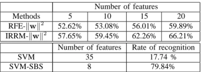
Methods 5 10 15 20 RFE-w2 52.62% 53.08% 56.01% 59.89% IRRM-w2 57.65% 59.45% 62.26% 66.21% Number of features Rate of recognition SVM 35 17.74 % SVM-SBS 8 79.84%
TABLE III
RESULTS OF VALENCE CLASSIFICATION
characteristic of the feature selection methods we tested, RFE and IRRM, the classification rates in tables show that the common SBS outperforms the other methods. Particularly, when comparing the number of selected features for each method, the superiority of the SBS method could be revealed more apparently. In the case of valence classification, we can see that the classification rate (79.84%) by using SBS differs extremely from the rate (17.74%) without selection method. This means that the more complex prediction problem such as valence classification, the more compact feature selection we need.
IV. CONCLUSION
In this paper, we tested different feature selection methods, SVM-RFE, SVM-IRRM, and the common SBS and compared the performance of the methods by recognition rates obtained from two binary emotion classifications, arousal and valence. It turned out that the SBS outperforms the other methods in both classification problems. Particularly, the work supports the general evidence that the arousal intensity of emotional states can be better classified than the valence classification, regardless which selection method is used.
REFERENCES
[1] I. Guyon and A. Elisseeff, “An introduction to variable and feature selection,” Journal of Machine Learning Research, pp. 1157–1182, 2003.
[2] A. Blum and P. Langley, “Selection of relevant features and examples in machine learning,” Artificial Intelligence, vol. 97, pp. 245–271, 1997.
[3] J. Weston, S. Mukherjee, O. Chapelle, M. Pontil, T. Poggio, and V. Vapnik, “Feature selection for svms,” in The Advances in Neural Information Processing Systems (NIPS), vol. 13, 2000, pp. 668–674.
[4] J. Wagner, J. Kim, and E. Andr´e, “From physiological signals to emotions: Implementing and comparing selected methods for feature extraction and classification,” in IEEE International Conf. on Multimedia and Expo (ICME’05), Amsterdam, The Netherlands, July 2005.
[5] N. Cristianini and J. Shawe-Taylor, Introduction to Support Vector Machine. Cambridge University Press, 2000.
5
[6] C. J. C. Burges, “A tutorial on support vector machines for pattern recognition,” Data Mining and Knowledge Discovery, vol. 2, no. 2, pp. 121–167, 1998.
[7] A. Rakotomamonjy, “Variable selection using svm-based crite-ria,” Journal of Machine Learning Research, vol. 3, pp. 1357– 1370, 2003.
[8] H. Froehlich and A. Zell, “Feature subset selection for support vector machines by incremental regularized risk minimization,” in IEEE Int. Joint Conf. on Neural Networks, vol. 3, July 2004, pp. 2041–2045.
[9] Y. Bengio, “Gradient-based optimization of hyperparameters,” Neural Computation, vol. 12, pp. 1989–1900, 2000.
[10] O. Chapelle, V. Vapnik, O. Bousquet, and S. Mukerjhee, “Choosing multiple parameters for svm,” Machine Learning, vol. 46, pp. 131–159, 2002.
[11] J. Kim, Robust Speech Recodgnition and Understanding. I-Tech Education and Publishing, Vienna, Austria, 2007, ch. Bimodal EMotion Recognition using Speech and Physiological Changes, pp. 265–280.