Quantitative Information Flow in Interactive Systems
M´ario S. Alvim1, Miguel E. Andr´es2, and Catuscia Palamidessi1. 1
INRIA and LIX, ´Ecole Polytechnique Palaiseau, France. 2Institute for Computing and Information Sciences, The Netherlands.
Abstract. We consider the problem of defining the information leakage in in-teractive systems where secrets and observables can alternate during the com-putation. We show that the information-theoretic approach which interprets such systems as (simple) noisy channels is no longer valid. However, the principle can be recovered if we consider channels of a more complicated kind, that in Infor-mation Theory are known as channels with memory and feedback. We show that there is a complete correspondence between interactive systems and such chan-nels. Furthermore, we show that the capacity of the channels associated to such systems is a continuous function with respect to a pseudometric based on the Kantorovich metric.
1
Introduction
Information leakage refers to the problem that arises when the observable behavior of a system reveals information that we would like to keep secret. This is also known as the problem of information flow from high variables to low variables. In recent years there has been a growing interest in quantitative approaches to this problem, because it is often desirable to quantify the partial knowledge of the secrets in terms of a probability distribution. Another reason is that the mechanisms to protect the information may use randomization to obfuscate the relation between the secrets and the observables.
Among the quantitative approaches, some of the most popular ones are based on In-formation Theory [5, 16, 4, 24, 6]. The idea is to interpret the system as an inIn-formation- information-theoretic channel, where the secrets are the input and the observables are the output. The channel matrix consists of the conditional probabilitiesp(b|a), defined as the measure of the executions producing the observableb, relative to those which contain the secret a. The leakage is represented by the mutual information, and the worst-case leakage by the capacity of the channel.
In the works cited above, the secret value is assumed to be chosen at the beginning of the computation. We are interested in the more general scenario in which secrets can be chosen at any point. More precisely, we consider interactive systems, i.e. systems in which the generation of secrets and the occurrence of observables can alternate during the computation and influence each other. Examples of interactive systems include
auc-tion protocols like [31, 27, 25]. Some of these have become very popular thanks to their
integration in Internet-based electronic commerce platforms [10, 11, 19]. Other exam-ples of interactive programs include web servers, GUI applications, and command-line programs [3].
In this paper we investigate the applicability of the information-theoretic approach to interactive systems. In order to derive an information-theoretic channel, at a first glance it would seem natural to define the channel matrix by using the definition of p(b|a)in terms of the joint and marginal probabilitiesp(a, b)andp(b). Namely, the entryp(b|a)would be defined as the measure of the traces with (secret, observable)-projection (a, b), divided by the measure of the traces with secret projection a. An approach of this kind was proposed in [9]. However, in the interactive case this con-struction does not really produce an information-theoretic channel. In fact, by definition a channel should be invariant with respect to the input distribution, and this is not the case here, as shown by the following example.
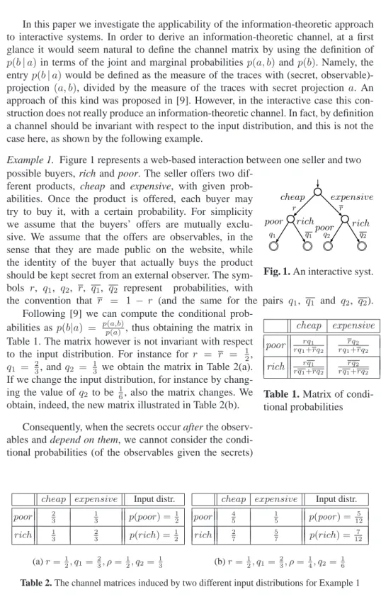
Example 1. Figure 1 represents a web-based interaction between one seller and two
cheap expensive poor rich
poor rich
r r
q1 q1 q2 q2
Fig. 1. An interactive syst.
possible buyers, rich and poor. The seller offers two dif-ferent products, cheap and expensive, with given prob-abilities. Once the product is offered, each buyer may try to buy it, with a certain probability. For simplicity we assume that the buyers’ offers are mutually exclu-sive. We assume that the offers are observables, in the sense that they are made public on the website, while the identity of the buyer that actually buys the product should be kept secret from an external observer. The sym-bols r, q1, q2, r, q1, q2 represent probabilities, with
the convention that r = 1 − r (and the same for the pairs q1, q1 and q2, q2). cheap expensive poor rq1 rq1+rq2 rq2 rq1+rq2 rich rq1 rq1+rq2 rq2 rq1+rq2
Table 1. Matrix of
condi-tional probabilities Following [9] we can compute the conditional
prob-abilities asp(b|a) = pp(a,b(a)), thus obtaining the matrix in Table 1. The matrix however is not invariant with respect to the input distribution. For instance for r = r = 12, q1 = 23, andq2 = 13 we obtain the matrix in Table 2(a). If we change the input distribution, for instance by chang-ing the value ofq2 to be 16, also the matrix changes. We obtain, indeed, the new matrix illustrated in Table 2(b).
Consequently, when the secrets occur after the observ-ables and depend on them, we cannot consider the condi-tional probabilities (of the observables given the secrets)
cheap expensive Input distr. poor 2 3 1 3 p(poor) = 1 2 rich 13 23 p(rich) = 12 (a)r=1 2, q1= 2 3, ρ= 1 2, q2= 1 3
cheap expensive Input distr. poor 4 5 1 5 p(poor) = 5 12 rich 27 57 p(rich) = 127 (b)r= 1 2, q1= 2 3, ρ= 1 4, q2= 1 6 Table 2. The channel matrices induced by two different input distributions for Example 1
as representing a classical channel from secrets to observables, and we cannot apply the standard information-theoretic concepts. In particular, we cannot use “the capacity of the matrix” (defined by considering the matrix as a channel matrix, and taking the max-imum mutual information over all possible inputs) because in general the maxmax-imum is given by a distribution different from the one that has originated the matrix, hence the result would be unsound.
The first contribution of this paper is to consider an extension of the theory of chan-nels which makes the information-theoretic approach applicable also the case of in-teractive systems. It turns out that a richer notion of channels, known in Information Theory as channels with memory and feedback, serves our purposes. The dependence of inputs on previous outputs corresponds to feedback, and the dependence of outputs on previous inputs and outputs corresponds to memory. Recent results in Information Theory [29] have shown that, in such channels, the transmission rate does not corre-spond to the maximum mutual information (the standard notion of capacity), but rather to the maximum normalized directed information, a concept introduced by Massey [17]. We propose to adopt this latter notion to represent leakage.
Our model of attacker is the interactive version of the attacker associated to Shannon entropy in the classification of K¨opf and Basin [15], based on an eavesdropper scenario. We recall that in [15] an attacker is defined by the kind of questions that he can pose to an hypothetical oracle. In the case of Shannon entropy the questions are of the form “doessbelong toS?” wheresis the secret that the attacker is trying to figure out, and Sis a subset of the domain of secret values. The degree of invulnerability of the secret is the average number of questions that the attacker needs to ask in order to find out the exact value of the secret, under the best strategy (i.e. the best choice of the S’s) for the given probability distribution on the secret values. It is easy to see that the invulnerabil-ity degree corresponds to the Shannon entropy of the secret. In the case of a standard single-use channel, the invulnerability degree of the secret before the attacker observes the output is the entropy of the input, determined by its a priori distribution. The invul-nerability degree after the attacker observes the output is the conditional entropy of the input given the output, determined by its a posteriori distribution. The latter is always smaller than or equal to the first. The difference between these invulnerability degrees corresponds to the mutual information, and represents the leakage of the system.
In our interactive framework we consider the same scenario, but iterated. At each time step, we consider the input sequence so far; and the increase of its vulnerability caused by the observation of the new output is given by the contribution of the present step to the leakage. The sum of all these contributions represents the total leakage and, as we will see, corresponds to Massey’s directed information. We will come back to the model of attacker in Section 5, and discuss also a variant of this interpretation.
Gray investigated a concept similar to directed information in [13]. In contrast to our model, which is based on an eavesdropper scenario, he considered leakage in a sender-receiver model. More precisely, he considered a system based on Millen’s synchronous state machine [20], and connected to “low” and “high” environments via communica-tion channels. His purpose was to measure the flow of informacommunica-tion from the high envi-ronment to the low one, assuming that the only way for the low envienvi-ronment to learn about the high one (and vice versa) is trough the system. To this end, he defined a
no-tion of “quasi-directed informano-tion” by extending Gallager’s formula for discrete finite state channels [12]. He also conjectured a correspondence between the quasi-directed information and the transmission rate of the channel. His formulation of quasi-directed information, however, is not completely the same as directed information, and as a result the conjecture does not hold. We come back to this point in Section 5, after Definition 9. A second contribution of our work is the proof that the channel capacity is a continu-ous function of a pseudometric on interactive systems based on the Kantorovich metric. The reason why we are interested in the continuity of the capacity is for computability purposes. Given a functionf from a (pseudo)metric spaceXto a (pseudo)metric space Y the continuity offmeans that, given a sequence of objectsx1, x2, . . .∈ X converg-ing tox∈ X, the sequencef(x1), f(x2), . . .∈ Y converges tof(x)∈ Y. Hencef(x) can be approximated by the objectsf(x1), f(x2), . . .. The typical use of this property is in the case of execution trees generated by programs containing loops. Generally the automaton expressing the semantics of the program can be seen as the (metric) limit of the sequence of trees generated by unfolding the loop at an increasingly deeper level. The continuity of the capacity means that we can approximate the real capacity by the capacities of these trees.
The continuity of the channel capacity was also proved in [9] for simple channels, but the proof does not adapt to the case of channels with memory and feedback and we had to devise a different technique. We illustrate this point by showing a counterexample (cfr. Example 6).
1.1 Plan of the paper
The paper is organized as follows. Section 2 reviews some important concepts from Probabilistic Automata and Information Theory. Section 3 reviews the notion of chan-nel with memory and feedback that is the core of the model we propose. We discuss the concept of directed information and also the concept of capacity in the presence of feed-back. Section 4 contains our main contribution. We explain how Interactive Information Hiding Systems (IIHSs) can be modeled using channels with memory and feedback. In particular we show that for any IIHS there is always a channel that simulates its prob-abilistic behavior. In Section 5 we discuss our notion of adversary and we define the quantification of information leakage as the channel’s directed information from input to output, or as the directed capacity, depending on whether the input distribution is fixed or not. In Section 6 we show an example of our model applied to a protocol: the Cocaine Auction protocol. Section 7 proposes a pseudometric structure on IIHSs based on the Kantorovich metric. We also show that the capacity of the channels associated to interactive systems is a continuous function with respect to this pseudometric. In Sec-tions 8 and 9 we review and discuss the main results of the paper and illustrate some future work.
A preliminary version of this paper appeared in the proceedings of CONCUR 2010 [1]. The additional material presented here consists in the proofs, the auxiliary Lem-mata 1, 2, and 3, Propositions 2 and 3, more examples, and a more elaborate discussion about the model.
2
Preliminaries
In this section we briefly review some basic notions that we will need throughout the paper.
2.1 Probabilistic automata
A functionµ: S →[0,1]is a discrete probability distribution on a countable setS if P
s∈Sµ(s) = 1andµ(s)≥0for alls. The set of all discrete probability distributions
onSisD(S).
A probabilistic automaton [22] is a quadrupleM = (S,L,ˆs, ϑ)whereSis a count-able set of states,La finite set of labels or actions,ˆsthe initial state, andϑa transition
functionϑ:S → ℘f(D(L × S)). Here℘f(X)is the set of all finite subsets ofX. If ϑ(s) =∅thensis a terminal state. We writes→µforµ∈ϑ(s), s∈ S. Moreover, we writes→ℓrfors, r∈ Swhenevers→µandµ(ℓ, r)>0. A fully probabilistic
automa-ton is a probabilistic automaautoma-ton satisfying|ϑ(s)| ≤ 1for all states. In such automata, whenϑ(s)6=∅, we overload the notation and denote byϑ(s)the distribution outgoing froms.
A path in a probabilistic automaton is a sequenceσ = s0 →ℓ1 s1 → · · ·ℓ2 where si ∈ S,ℓi ∈ Landsiℓi+1
→si+1. A path can be finite in which case it ends with a state. A path is complete if it is either infinite, or finite ending in a terminal state. Given a finite pathσ,last(σ)denotes its last state. LetPathss(M)denote the set of all paths, Paths⋆
s(M)the set of all finite paths, andCPathss(M)the set of all complete paths of an automatonM, starting from the states. We will omitsifs= ˆs. Paths are ordered by the prefix relation, which we denote by≤. The trace of a path is the sequence of actions inL∗∪ L∞obtained by removing the states, hence for the aboveσwe have
trace(σ) = l1l2. . .. IfL′ ⊆ L, thentraceL′(σ)is the projection oftrace(σ)on the
elements ofL′.
LetM = (S,L,s, ϑˆ )be a (fully) probabilistic automaton,s ∈ S a state, and let σ ∈ Paths⋆s(M)be a finite path starting in s. The cone generated byσis the set of complete pathshσi = {σ′ ∈ CPaths
s(M) | σ ≤ σ′}. Given a fully probabilistic automaton M = (S,L,s, ϑˆ )and a state s, we can calculate the probability value, denoted byPs(σ), of any finite pathσstarting insas follows:Ps(s) = 1andPs(σ
ℓ
→
s′) =P
s(σ)µ(ℓ, s′), where last(σ)→µ.
LetΩs ,CPathss(M)be the sample space, and letFsbe the smallestσ-algebra induced by the cones generated by all the finite paths ofM. ThenPinduces a unique
probability measure on Fs (which we will also denote byPs) such that Ps(hσi) = Ps(σ)for every finite pathσstarting ins. Fors= ˆswe writePinstead ofPˆs.
Given a probability space(Ω,F, P)and two eventsA, B∈ FwithP(B)>0, the
conditional probability ofAgivenB,P(A|B), is defined asP(A∩B)/P(B).
2.2 Concepts from Information Theory
For more detailed information on this part we refer to [7]. LetA, B denote two dis-crete random variables with finitely many values, and with corresponding probability
distributionspA(·), pB(·), respectively (we shall omit the subscripts when they are clear from the context). LetA={a1, . . . , an},B ={b1, . . . , bm}denote, respectively, the sets of possible values forAand forB.
The entropy of A is defined as H(A) = −P
Ap(a) logp(a) and it measures
the uncertainty of A. It takes its minimum valueH(A) = 0 when pA(·)is a point mass (also called delta of Dirac). The maximum valueH(A) = log|A| is obtained when pA(·) is the uniform distribution. Usually the base of the logarithm is set to be 2 and the entropy is measured in bits. The conditional entropy of A givenB is H(A|B) = −P
Bp(b)
P
Ap(a|b) logp(a|b), and it measures the uncertainty of A
whenBis known. It is well-known that0 ≤H(A|B)≤H(A). The minimum value, 0, is obtained whenAis completely determined byB. The maximum valueH(A)is obtained whenAandB are independent. The mutual information betweenAandBis defined asI(A;B) = H(A)−H(A|B), and it measures the amount of information aboutAthat we gain by observing B. It can be shown thatI(A;B) = I(B;A)and 0≤I(A;B)≤H(A). IfCis a third random variable, the conditional mutual
informa-tion betweenAandBgivenCis defined asI(A;B|C) =H(A|C)−H(A|B, C). The (conditional) entropy and mutual information respect the chain rules. Namely, given the random variablesA1, A2, . . . , Ak,BandC, we have:
H(A1, A2, . . . , Ak|C) = k X i=1 H(Ai|A1, . . . , Ai−1, C) (1) I(A1, A2, . . . , Ak;B|C) = k X i=1 I(Ai;B|A1, . . . , Ai−1, C) (2) A (discrete memoryless) channel is a tuple(A,B, p(·|·)), whereA,Bare the sets of input and output symbols, respectively, andp(b|a)is the probability of observing the output symbolbwhen the input symbol isa. These conditional probabilities constitute the channel matrix. An input distributionpA(·)overAtogether with the channel de-termine the joint distributionp(a, b) = p(a|b)·p(a)and consequentlyI(A;B). The maximumI(A;B)over all possible input distributions is the channel’s capacity. Fi-nally, a family ρ = {pv(·)}v of probability measures parametrized onv is called a
stochastic kernel1.
3
Discrete channels with memory and feedback
In this section we present the notion of channel with memory and feedback. We assume a scenario in which the channel is used repeatedly, in a finite temporal sequence of steps 1, . . . , T. Intuitively, memory means that the output at timetdepends on the input and output histories, i.e. on the inputs up to time t, and on the output up to time t−1. Feedback means that the input at timetdepends on the outputs up to timet−1.
We adopt the following notation, which appears to be standard in the literature of channels with memory and feedback.
1
The general definition of stochastic kernel is more complicated (cfr. [29]), but it reduces to this one in the case of discrete channels, which is what we use in this paper.
Convention 1. Given a set of symbols (alphabet)A={a1, . . . , an}, we use a Greek letter (α,β, . . . ) to denote a sequence of symbols ordered in time. Given a sequence
α =ai1ai2. . . aim, the notationαtrepresents the symbol at timet, i.e. ait, whileα
t
represents the sequenceαi1αi2. . . αit. For instance, in the sequenceα=a3a7a5, we
haveα2=a7andα2=a3a7. Analogously, ifXis a random variable, thenXtdenotes
the sequence oftconsecutive instancesX1, . . . , XtofX.
We now define formally the concepts of memory and feedback. Consider a channel from inputAto outputB. The channel behavior afterT uses can be fully described by the joint distribution ofAT ×BT, namely by the probabilitiesp(αT, βT). Using the chain rule, we can decompose these probabilities as follows:
p(αT, βT) = T Y t=1 p(αt|αt−1, βt−1)p(β t|αt, βt−1) (3)
Definition 1. We say that the channel has feedback if, in general,p(αt|αt−1, βt−1)6= p(αt|αt−1), i.e. the probability of αt depends not only on αt−1, but also on βt−1.
Analogously, we say that the channel has memory if, in general, p(βt|αt, βt−1) 6= p(βt|αt), i.e. the probability ofβtdepends onαtandβt−1.
Note that in the opposite case, i.e. whenp(αt|αt−1, βt−1)coincides withp(αt|αt−1) andp(βt|αt, βt−1)coincides withp(β
t|αt), then we have a classical channel (mem-oryless, and without feedback), in which each use is independent from the previous ones. The only possible dependency on the history is the one ofaton at−1. This is because A1, . . . , AT are in general correlated, due to the fact that they are produced by an encoding function. Note that in absence of memory and feedback (3) reduces to p(αT, βT) =QT
t=1p(αt|αt−1)p(βt|αt), which is the standard formula for a classical channel afterT uses.
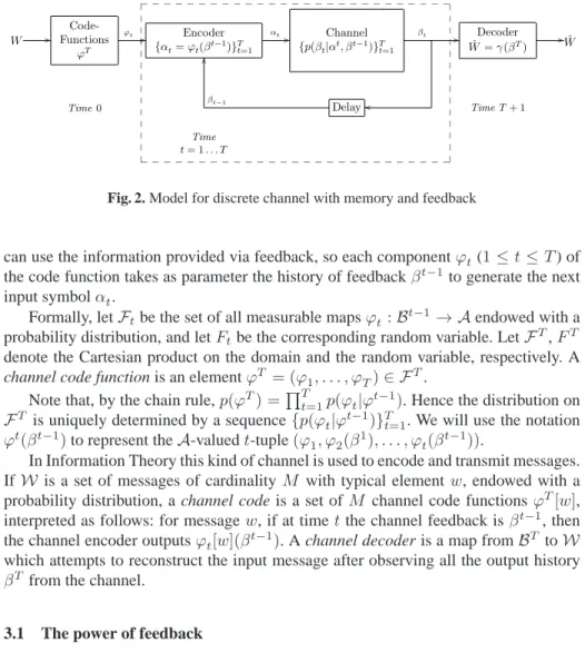
The above is a very abstract description of a channel with memory and feedback. We now discuss a more concrete notion following the presentation of [29] . Such a channel, represented in Figure 2, consists of a sequence of components formally de-fined as a family of stochastic kernels{p(· |αt, βt−1)}T
t=1 overB. The probabilities p(βt|αt, βt−1)represent the innermost behavior of the channel at timet,1≤t ≤T: the internal channel takes the inputαtand, depending on the history of inputs and out-puts so far, it produces an output symbolβt. The output is then fed back to the encoder with delay one. On the output side, at time tthe encoder takes the message and the past output symbolsβt−1and produces a channel input symbolα
taccording to a code functionϕt(we will explain this concept in the next paragraph). At final timeT the decoder takes all the channel outputsβT and produces the decoded messageWˆ. The order is the following:
Message W, α1, β1, α2, β2, . . . , αT, βT, Decoded Message Wˆ (4) Let us now explain the concept of code function. Intuitively, a code function is a strategy to encode the message into a suitable representation to be transmitted through the channel. There is a code function for each possible message, and the function is fixed at the very beginning of the transmission (time t = 0). However, the encoding
W // Code-Functions ϕT ϕt / / Encoder {αt=ϕt(βt−1)}Tt=1 αt / / Channel {p(βt|αt, βt−1)}Tt=1 βt / / o o Decoder ˆ W=γ(βT) //Wˆ Time0 βt−1 Delay O O TimeT+ 1 __ __ __ __ __ __ __ ___ __ __ __ __ __ __ __ __ __ __ __ __ ___ __ __ __ __ __ Time t= 1. . . T
Fig. 2. Model for discrete channel with memory and feedback
can use the information provided via feedback, so each componentϕt(1≤t≤T) of the code function takes as parameter the history of feedbackβt−1to generate the next input symbolαt.
Formally, letFtbe the set of all measurable mapsϕt:Bt−1→ Aendowed with a probability distribution, and letFtbe the corresponding random variable. LetFT,FT denote the Cartesian product on the domain and the random variable, respectively. A
channel code function is an elementϕT = (ϕ
1, . . . , ϕT)∈ FT. Note that, by the chain rule,p(ϕT) =QT
t=1p(ϕt|ϕt−1). Hence the distribution on
FT is uniquely determined by a sequence{p(ϕ
t|ϕt−1)}Tt=1. We will use the notation ϕt(βt−1)to represent theA-valuedt-tuple(ϕ
1, ϕ2(β1), . . . , ϕt(βt−1)).
In Information Theory this kind of channel is used to encode and transmit messages. IfW is a set of messages of cardinality M with typical elementw, endowed with a probability distribution, a channel code is a set ofM channel code functions ϕT[w], interpreted as follows: for messagew, if at timet the channel feedback isβt−1, then the channel encoder outputsϕt[w](βt−1). A channel decoder is a map fromBT toW which attempts to reconstruct the input message after observing all the output history βT from the channel.
3.1 The power of feedback
The original purpose of communication channel models is to represent data transmis-sion from a source to a receiver. Shannon’s Channel Coding Theorem states for every channel there is an encoding scheme that allows a transmission rate arbitrarily close to the channel capacity with a negligible probability of error (if the number of uses of the channel is large enough). A general way to find an optimal encoding scheme that is also easy to decode has not been found yet. The use of feedback, however, can simplify the design of both the encoder and the decoder. The following example illustrates the idea.
Example 2. Consider a discrete memoryless binary channel {A,B, p(.|.)} withA =
{0,1},B={0,1,e}and the channel matrix of Table 3.
0 1 e
0 0.8 0 0.2 1 0 0.8 0.2
Table 3. Channel
ma-trix for binary erasure This kind of channel is called erasure channel because it
can lose (or erase) bits during the transmission with a certain
probability. Namely, any bit has0.8probability of being cor-rectly transmitted, and 0.2 probability of being lost. On the output side the encoder is able to detect whether the bit was erased (by receiving anesymbol), but it cannot tell which was the actual value of the original bit. The Channel Coding The-orem guarantees that the maximum information transmission rate in this channel is (2to the power of) the channel capacity, i.e0.8bits per use of the channel.
Following simple principles described in [7], an encoding that achieves the capac-ity can be easily obtained if the channel can be used with feedback. The idea is an adaptation of the stop-and-wait protocol [26, 28]. Suppose that every bit received on the output end of the channel is fed back noiselessly to the source with delay1. Define the encoding as follows: for each bit transmitted, the encoder checks via feedback if the bit was erased. If not, the encoder moves on to transmit the next of the message. If yes, the encoder transmits the same bit again.
It is easy to see that with this encoding scheme the transmission rate is0.8bit per usage of the channel, since in80%of the cases the bit is transmitted properly, and in 20%it is lost and a retransmission is needed.
In Appendix A we come back to this example to illustrate in more detail the design and the function of the encoder and decoder. Note that the channel capacity in the above example does not increase with the addition of feedback (it is0.8bit per usage of the channel with or without feedback). This is because the channel is memoryless: feedback
does not increase the capacity of discrete memoryless channels [7]. In general however,
feedback does increase the capacity.
3.2 Directed information and capacity of channels with feedback
In classical Information Theory, the channel capacity, which is related to the channel’s transmission rate by Shannon’s Channel Coding Theorem, can be obtained as the supre-mum of the mutual information over all possible input distributions. In the presence of feedback, however, this correspondence no longer holds. More specifically, mutual in-formation no longer represents the inin-formation flow fromAT toBT. Intuitively, this is due to the fact that mutual information expresses correlation, and therefore it is creased by feedback (see Example 5). However, feedback, i.e the way the output in-fluences the next input, is not part of the information to be transmitted. If we want to maintain the correspondence between the transmission rate and capacity, we need to replace the mutual information with directed information [17].
Definition 2. In a channel with feedback, the directed information from input AT to
output BT is defined as I(AT → BT) = PT
t=1I(At;Bt|Bt−1). In the other
di-rection, the directed information from BT toAT is defined as: I(BT → AT) = PT
t=1I(At;Bt−1|At−1).
In Section 5 we shall discuss the relation between directed information and mutual information, as well as the correspondence with information leakage. For the moment, we only present the extension of the concept of capacity.
LetDT ={{p(αt|αt−1, βt−1)}Tt=1}be the set of all input distributions in presence of feedback. For finiteT, the capacity of a channel with memory and feedback is:
CT = sup
DT
1 TI(A
T →BT) (5)
The capacity is also defined when T is infinite, see [29]. However in this paper we consider only the finite case.
4
Interactive systems as channels with memory and feedback
Interactive Information Hiding Systems (IIHS) were introduced in [2] to represent systems where secrets (inputs) and observable (outputs) can interleave and influence each other. They are a variant of probabilistic automata in which actions are divided in secrets and observables. They can be of two kinds: fully probabilistic, andsecret-nondeterministic (or input-secret-nondeterministic). In the former there is no nondeterminism,
while in the latter every secret choice is fully nondeterministic.
In this paper we consider normalized IIHSs, in which secrets and observables al-ternate, and the actions at the first level are secrets. We note that this is not really a restriction, because given an IIHS which is not normalized, it is always possible to transform it into a normalized IIHS which is equivalent to the former one up to a given execution level. The reader can find in Appendix B the formal definition of the transfor-mation. Furthermore, we require that for each statesand each actionℓthere is at most one state that can be reached fromsby performing anℓtransition.
We give now the formal definition of the kind of IIHSs that we will use in this paper.
Definition 3. A (normalized) IIHS is a triple I = (M,A,B), where A and B are disjoint sets of secrets and observables respectively, M is a probabilistic automaton
(S,L,ˆs, ϑ)withL=A ∪ B, and, for eachs∈ S:
1. eitherϑ(s)⊆ D(A × S)orϑ(s)⊆ D(B × S). We callsa secret state in the first
case, and an observable state in the second case;
2. ifs→ℓ rthen: if sis a secret state then r is an observable state, and ifs is an observable state thenris a secret state;
3. ˆs is a secret state;
4. ifsis an observable state then|ϑ(s)| ≤1; 5. either:
(i) for every secret stateswe have|ϑ(s)| ≤1(fully probabilistic IIHS),
or
(ii) for every secret statesthere existai andsi (i = 1, . . . , n) such thatϑ(s) =
{δ(ai, si)}n
i=1, whereδ(ai, si)is the Dirac measure (secret-nondeterministic IIHS);
6. for every statesand actionℓthere exists a unique statersuch thats→ℓ r.
In the rest of the paper we will omit the adjective “normalized” for simplicity. In the above definition, Conditions 1 and 2 imply that the IIHS is alternating between secrets and observables. Moreover, all the transitions between nodes at two consecutive depths
have either secret actions only, or observable actions only. Condition 3 means that the first level contains secret actions. Condition 4 means that all observable transitions are fully probabilistic. Condition 5 means that all secret transitions are either fully prob-abilistic or fully nondeterministic. The term “nondeterministic” is justified by the fact that the scheme of Condition 5(ii), represented in Figure 3(a), is equivalent to the one of Figure 3(b). s rj1 rjj rjn r11 r1n rn1 rnn . . . . . . . . . . . . . . a1 0 aj 1 an 0 a1 1 an 0 a1 0 an 1
(a) Nondeterministic input using Dirac measures
s r11 rjj rnn · · · · a1 aj an (b) Equivalent scheme Fig. 3. Scheme of secret transitions for secret-nondeterministic IIHSs.
Note that we do not consider here internal nondeterminism such as that one arising from interleaving of concurrent processes. This means that we make a rather restricted use of probabilistic automata, but this is enough for our purposes. The nondeterminism generated by concurrency gives rise to a new set of problems (see for example [4]) which are orthogonal to those considered in this paper.
Condition 6 means that the secret and observable actions determine the states. As a consequence, the actions are enough to retrieve the path. This is expressed by the following proposition:
Proposition 1. Given an IIHS, consider two pathsσandσ′. Iftrace
A(σ) =traceA(σ′) andtraceB(σ) =traceB(σ′), thenσ=σ′.
Proof. By induction on the length of the traces. The initial state of the automaton is
uniquely determined by the empty (secret and observable) traces. Assume now we are in a statesuniquely determined by secret and observable tracesαandβ, respectively. Ifs makes a secret transitions→a s′, then by Condition 6 there is only one states′reachable
fromsvia ana-transition, and therefores′ is uniquely determined by the secret trace
α′=αaand the observable traceβ. The case in whichsmakes an observable transition
is similar.
4.1 Construction of the channel associated to an IIHS
We now show how to associate a channel to an IIHS.
In an interactive system secrets and observables may interleave and influence each other. Considering a channel with memory and feedback is a way to capture this rich
behavior. Secrets have a causal influence on observables via the channel, and, in the presence of interactivity, observables have a causal influence on secrets via feedback. This alternating mutual influence between secrets and observables can be modeled by repeated uses of the channel. Each time the channel is used it represents a different state of the computation, and the conditional probabilities of observables with respect to secrets can depend on this state. The addition of memory to the model allows expressing the dependency of the channel matrix on such a state.
We will see that a secret-nondeterministic IIHS determines a channel as specified by its stochastic kernel, while a fully probabilistic IIHS determines, additionally, the input distribution. In Section 6 we will give an extensive and detailed example of how to make such a construction for a real security protocol.
Given a pathσof length2t−1, we will denotetraceA(σ)byαt, andtraceB(σ)by
βt−1.
Definition 4. LetIbe an IIHS. For eacht, the channel’s stochastic kernel correspond-ing toIis defined asp(β
t|αt, βt−1) =ϑ(s)(βt, s′), wheresis the state reached from
the root via the pathσwhose secret and observable traces areαtandβt−1respectively. Note thatsands′in the previous definition are well defined: by Proposition 1,sis
unique, and since the choice ofβtis fully probabilistic,s′is also unique.
The following example illustrates how to apply Definition 4, with the help of Propo-sition 1, to build the channel matrix of a simple example.
Example 3. Let us consider an extended version of the website interactive system of
Figure 1. We maintain the general definition of the system, i.e, there are two possi-ble buyers (richandpoorrepresented byrc.andpr., respectively) and two possible products (cheapandexpensive, represented bychp.andexp., respectively). We still assume that offers are observable, since they are visible to everyone on the website, but the identity of buyers should be kept secret. We consider two consecutive rounds of offers and buys, which implies that, after normalization,T = 3. Figure 4 shows an automaton for this example in normalized form. Transitions with null probability are omitted, and the symbola∗ is used as a place holder to achieve the normalized IIHS
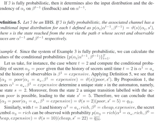
(see Appendix).
To construct the stochastic kernels{p(βt|αt, βt−1)}Tt=1, we need to determine the conditional probability of an observable at timetgiven the history up to timet.
Let us take the caset= 2and compute the conditional probability of the observable β2 = cheapgiven that the history of secrets until timet = 2isα2 = a∗, poorand
the history of observables is β1 = expensive. Applying Definition 4, we see that p(β2=cheap|α2=a∗, poor, β1=expensive) =ϑ(s)(cheap, s′). By Proposition 1,
the tracesα2=a
∗, poor, β1=expensivedetermine a unique statesin the automaton,
namely, the states= 5. Moreover, from the state5a unique transition labelled with the actioncheapis possible, leading to the states′ = 11. Therefore, we can conclude that
p(β2=cheap|α2=a∗, poor, β1=expensive) =ϑ(s= 5)(cheap, s′= 11) =p23. Similarly, witht = 1and historyα1 =a
∗, β0 = ǫ, the observable symbolβ1 = expensivecan be observed with probabilityp(β1 =expensive|α1 =a∗, β0=ǫ) =
ϑ(s= 0)(cheap, s′= 2) =p
IfIis fully probabilistic, then it determines also the input distribution and the de-pendency ofαtonβt−1(feedback) and onαt−1.
Definition 5. LetIbe an IIHS. IfIis fully probabilistic, the associated channel has a conditional input distribution for eachtdefined as p(αt|αt−1, βt−1) = ϑ(s)(α
t, s′),
wheresis the state reached from the root via the pathσwhose secret and observable traces areαt−1andβt−1respectively.
Example 4. Since the system of Example 3 is fully probabilistic, we can calculate the
values of the conditional probabilities{p(αt|αt−1, βt−1)}T t=1.
Let us take, for instance, the case wheret= 2and compute the conditional proba-bility of secretα2=poorgiven that the history of secrets until timet= 2isα1=a∗
and the history of observables isβ1=expensive. Applying Definition 5, we see that p(α2 = poor|α1 = a∗, β1 = expensive) = ϑ(s)(poor, s′). By Proposition 1, the
tracesα1 =a
∗, β1=expensivedetermine a unique statesin the automaton, namely,
the states = 2. Moreover, from the state2 a unique transition labelled with the ac-tion poor is possible, leading to the state s′ = 5. Therefore, we can conclude that p(α2=poor|α1=a∗, β1=expensive) =ϑ(s= 2)(poor, s′= 5) =q
12. Similarly, witht= 3and historyα2=a
∗, rich, β2=cheap, expensive, the secret
symbolα3=richcan be observed with probabilityp(α3=rich|α2=α∗, rich, β0=
cheap, expensive) =ϑ(s= 10)(cheap, s′= 22) =q
24. −1 0 1 2 3 4 5 6 7 8 9 10 11 12 13 14 15 16 17 18 19 20 21 22 23 24 25 26 27 28 29 30 31 32 33 34 35 36 37 38 39 40 41 42 43 44 45 46 a∗ chp. exp. pr. rc. pr. rc.
chp. exp. chp. exp. chp. exp. chp. exp.
pr. rc. pr. rc. pr. rc. pr. rc. pr. rc. pr. rc. pr. rc. pr. rc. b∗ b∗ b∗ b∗ b∗ b∗ b∗ b∗ b∗ b∗ b∗ b∗ b∗ b∗ b∗ b∗ 1 p1 p1 q11 q11 q12 q12 p21 p21 p22 p22 p23 p23 p24 p24 q21 q21q22 q22q23 q23q24 q24q25 q25q26 q26q27 q27q28 q28 1 1 1 1 1 1 1 1 1 1 1 1 1 1 1 1
4.2 Lifting the channel inputs to reaction functions
Definitions 4 and 5 show how to obtain the the joint probabilitiesp(αt, βt)for a fully probabilistic IIHS. We still need to show in what sense this joint probability distribution defines an information-theoretic channel.
The{p(βt|αt, βt−1)}Tt=1determined by the IIHS correspond to a channel’s stochas-tic kernel. The problem resides in the conditional probabilities{p(αt|αt−1, βt−1)}Tt=1. In an information-theoretic channel, the value of αt is determined in the encoder by a deterministic functionϕt(βt−1). Therefore, inside the encoder there is no possibil-ity for a probabilistic description ofαt. The solution is to externalize this probabilistic behavior to the code functions.
As shown in [29], the original channel with feedback from input symbolsAT to output symbolsBT can be lifted to an equivalent channel without feedback from code functionsFT to output symbolsBT. This transformation also allows us to calculate the channel capacity. Let{p(ϕt|ϕt−1)}T
t=1be a sequence of code function stochastic ker-nels and let{p(βt|αt, βt−1)}T
t=1be a channel with memory and feedback. The channel fromFT toBT is constructed using a joint measureQ(ϕT, αT, βT)that respects the following constraints:
Definition 6. A measure Q(ϕT, αT, βT)is said to be consistent with respect to the
code function stochastic kernels{p(ϕt|ϕt−1)}T
t=1and the channel{p(βt|αt, βt−1)}Tt=1
if, for eacht:
1. There is no feedback to the code functions:Q(ϕt|ϕt−1, αt−1, βt−1) =p(ϕ t|ϕt−1).
2. The input is a function of the past outputs:Q(αt|ϕt, αt−1, βt−1) =δ{ϕt(βt−1)}(αt)
whereδis the Dirac measure.
3. The properties of the underlying channel are preserved:
Q(βt|Ft=ϕt, At=αt, Bt−1=βt−1) =p(βt|αt, βt−1)
The following result states that there is only one consistent measureQ(ϕT, αT, βT):
Theorem 2 ([29]). Given{p(ϕt|ϕt−1)}T
t=1 and a channel{p(βt|αt, βt−1)}Tt=1, there
exists only one consistent measureQ(ϕT, αT, βT). Furthermore the channel fromFT
toBT is given by:
Q(βt|ϕt, βt−1) =p(β t|ϕt(βt
−1), βt−1) (6) Since in our setting the concept of encoder makes little sense as there is no in-formation to encode, we externalize the probabilistic behavior ofαtas follows. Code functions become a single set of reaction functions {ϕt}T
t=1 withβt−1 as parameter (the messagewdoes not play a role any more). Reaction functions can be seen as a model of how the environment reacts to given system outputs, producing new system inputs (they do not play a role of encoding a message). These reaction functions are endowed with a probability distribution that generates the probabilistic behavior of the values ofαt.
Definition 7. A reactor is a distribution on reaction functions, i.e., a sequence of stochas-tic kernels{p(ϕt|ϕt−1)}T
if it induces the compatible distributionQ(ϕT, αT, βT)such that, for every1≤t≤T, Q(αt|αt−1, βt−1) = p(α
t|αt−1, βt−1), where the latter is the probability distribution
induced byI.
The main result of this section states that for any fully probabilistic IIHS there is a reactor that generates the probabilistic behavior of the IIHS.
Lemma 1. LetX,Ybe non-empty finite sets, and letx˜∈ X,y˜∈ Y. Letp:X × Y →
[0,1]be a function such that, for everyx∈ X, we have:P
y∈Yp(x, y) = 1. Then: X f∈X →Y f(˜x)=˜y Y x∈X p(x, f(x)) =p(˜x,y˜)
Proof. By induction on the number of elements ofX.
Base case: X ={x˜}. In this case: X f∈X →Y f(˜x)=˜y Y x∈X p(x, f(x)) =p(˜x, f(˜x)) =p(˜x,y˜)
Inductive case: LetX =X′∪ {˚x}, with˜x∈ X′and˚x /∈ X′. Then:
X f∈X′∪{˚x}→Y f(˜x)=˜y Y x∈X′∪{˚x} p(x, f(x)) = (by distributivity) X f∈X′→Y f(˜x)=˜y Y x∈X′ p(x, f(x)) · X g∈{˚x}→Y p(˚x, g(˚x))
= (by the assumption) X f∈X′→Y f(˜x)=˜y Y x∈X′ p(x, f(x))
= (by the induction hypothesis) p(˜x,y˜)
Theorem 3. LetIbe a fully probabilistic IIHS inducing the joint probability distribu-tionp(αt, βt),1 ≤ t ≤ T, on secret and observable traces. It is always possible to
construct a channel with memory and feedback, and an associated probability distribu-tionQ(ϕT, αT, βT), which corresponds toIin the sense that, for every1≤t≤T,αt, βt, the equalityQ(αt, βt) =p(αt, βt)holds.
Proof. First of all we note that, by the laws of probability,Q(αt, βt) =P
ϕtQ(ϕt, αt, βt).
So we need to show thatP
ϕtQ(ϕt, αt, βt) =p(αt, βt)by induction ont.
Base case: t = 1. Let us defineQ(ϕ1|ǫ) = p(ϕ1(ǫ))andQ(β1|α1, ǫ) = p(β1|α1). Then: X ϕ1 Q(ϕ1, α1, β1) =X ϕ1 Q(ϕ1, α1, β1) =X ϕ1
Q(ϕ1|ǫ, ǫ, ǫ)Q(α1|ϕ1, ǫ, ǫ)Q(β1|ϕ1, α1, ǫ)(by the chain rule) =X ϕ1 Q(ϕ1|ǫ)δ{ϕ1(ǫ)}(α1)Q(β1|α 1, ǫ) (by Definition 6) =X ϕ1 p(ϕ1(ǫ))δ{ϕ1(ǫ)}(α1)p(β1|α1) (by construction ofQ) =p(α1)p(β1|α1) (by definition ofδ) =p(α1, β1) =p(α1, β1)
Inductive case: Let us defineQ(βt|αt, βt−1) =p(β
t|αt, βt−1), and
Q(ϕt|ϕt−1) = Y βt−1
p(ϕt(βt−1)|ϕt−1(βt−2), βt−1)
Note that, if we considerX = {βt−1 | β
i ∈ B,1 ≤ i ≤ t−1},Y = A, and p(βt−1, α
t) =p(αt|ϕt−1(βt−2), βt−1), thenX,Yandpsatisfy the hypothesis of Lemma 1.
Then: X
ϕt
Q(ϕt, αt, βt) = (by the chain rule) X ϕt Q(ϕt−1, αt−1, βt−1)Q(ϕt|ϕt−1, αt−1, βt−1)Q(αt|ϕt, αt−1, βt−1)Q(βt|ϕt, αt, βt−1) = (by Definition 6) X ϕt Q(ϕt−1, αt−1, βt−1)Q(ϕt|ϕt−1)δ{ϕt(βt−1)}(αt)Q(βt|α t, βt−1) = (by construction ofQ) X ϕt Q(ϕt−1, αt−1, βt−1) Y β′t−1 p(ϕt(β′t−1)|ϕt−1(β′t−2 ), β′t−1) δ{ϕt(βt−1)}(αt)p(βt|α t, βt−1) = (by definition ofδ) X ϕt ϕt(βt− 1)= αt Q(ϕt−1, αt−1, βt−1) Y β′t−1 p(ϕt(β′t−1)|ϕt−1(β′t−2 ), β′t−1) p(βt|αt, βt−1) = X ϕt−1 Q(ϕt−1, αt−1, βt−1)p(β t|αt, βt−1) X ϕt ϕt(βt− 1 )=αt Y β′t−1 p(ϕt(β′t−1)|ϕt−1(β′t−2 ), β′t−1) = (by Lemma 1) X ϕt−1 Q(ϕt−1, αt−1, βt−1)·p(β t|αt, βt−1)·p(αt|αt−1, βt−1) = p(βt|αt, βt−1)·p(αt|αt−1, βt−1)· X ϕt−1 Q(ϕt−1, αt−1, βt−1) = (by induction hypothesis)
p(βt|αt, βt−1)·p(α t|αt
−1, βt−1)·p(αt−1, βt−1) = (by the chain rule)
p(αt, βt)
Corollary 1. LetIbe a fully probabilistic IIHS. Let{p(β
t|αt, βt−1)}Tt=1be a sequence
of stochastic kernels and{p(αt|αt−1, βt−1)}T
t=1a sequence of input distributions
de-fined byI according to Definitions 4 and 5. Then the reactorR = {p(ϕ
t|ϕt−1)}Tt=1
p(ϕ1) =p(α1|α0, β0) =p(α1) (7) p(ϕt|ϕt−1) = Y
βt−1
p(ϕt(βt−1)|ϕt−1(βt−2), βt−1), 2≤t≤T (8)
Figure 5 depicts the model for IIHS. Note that, in relation to Figure 2, there are some simplifications: (1) no messagewis needed; (2) the encoder becomes an “interactor”; (3) the decoder is not used. At the beginning, a reaction function sequenceϕT is chosen and then the channel is usedT times. At each usaget, the interactor produces the next input symbolαtby applying the reaction functionϕtto the fed back outputβt−1. Then the channel produces an outputβtbased on the stochastic kernelp(βt|αt, βt−1). The output is then fed back to the encoder, which uses it for producing the next input.
Reaction-Functions ϕT ϕt / / “Interactor” {αt=ϕt(βt−1)}Tt=1 αt / / Channel {p(βt|αt, βt−1)}Tt=1 βt / / o o Delay βt−1 O O ___ ____ _____ ____ ____ _____ __ ___ ____ _____ ____ ____ _____ __
Fig. 5. Channel with memory and feedback model for IIHS
We conclude this section by remarking on an intriguing coincidence: The notion of reaction function sequenceϕT, on the IIHSs, corresponds to the notion of deterministic scheduler [22]. In fact, each reaction functionϕtselects the next step,αt, on the basis of theβt−1andαt−1(generated byϕt−1), andβt−1,αt−1represent the path until that state.
5
Leakage in Interactive Systems
In this section we propose a definition for the notion of leakage in interactive systems. We first argue that mutual information is not the correct notion, and we propose to replace it with the directed information instead.
In the case of channels with memory and feedback, mutual information is defined asI(AT;BT) = H(AT)−H(AT|BT), and it is still symmetric (i.e.I(AT;BT) = I(BT;AT)). Since the roles of AT andBT inI(AT;BT)are interchangeable, this concept cannot capture causality, in the sense that it does not imply that AT causes BT, nor conversely. Mutual information expresses correlation between the sequences of random variablesAT andBT.
Mathematically, forT usages of the channel, the mutual information I(AT;BT) can be expressed with the help of the chain rule of (2) in the following form.
I(AT;BT) = T X
t=1
I(AT;Bt|Bt−1) (9)
In the equation above, each term of the sum is the mutual information between the random variableBtand the whole sequence of random variablesAT =A
1, . . . , AT, given the history Bt−1. The equation emphasizes that at time1≤t≤T, even though only the inputsαt =α
1, α2, . . . , αthave been fed to the channel, the whole sequence AT, includingAt
+1, At+2, . . . , AT, has a statistical correlation with Bt. Indeed, in the presence of feedback,Btmay influenceAt+1, At+2, . . . , AT.
In order to show how the concept of directed information contrasts with the above, let us recall its definition:
I(AT →BT) = T X t=1 I(At;Bt|Bt−1). I(BT →AT) = T X t=1 I(At;Bt−1|At−1).
These notions capture the concept of causality, to which the definition of mutual in-formation is indifferent. The correlation between inputs and outputsI(AT;BT)is split into the informationI(AT →BT)that flows from input to output through the channel and the information I(BT → AT)that flows from output to the input via feedback. Note that the directed information is not symmetric: the flow fromAT toBT takes into account the correlation betweenAtandBt, while the flow fromBT toAT takes into account the correlation betweenBt−1andAt.
It was proved in [29] that
I(AT;BT) =I(AT →BT) +I(BT →AT) (10) i.e, the mutual information is the sum of the directed information flow in both senses. Note that this formulation highlights the symmetry of mutual information from yet another perspective.
Once we split mutual information into directed information in the two opposite directions, it is important to understand the different roles that the information flow in each direction plays. I(AT →BT)represents the system behavior: via the channel the information flows from inputs to outputs according to the system specification, modeled by the channel stochastic kernels. This flow represents the amount of information an attacker can gain from the inputs by observing the outputs, and we argue that this is the real information leakage.
On the other hand,I(BT → AT) represents how the environment reacts to the system: given the system outputs, the environment produces new inputs. We argue that the information flow from outputs to inputs is independent of any particular system: it is a characteristic of the environment itself. Hence, if an attacker knows how the en-vironment reacts to outputs, i.e the probabilistic behavior of the enen-vironment reactions
given the system outputs, this knowledge is part of the a priori knowledge of the adver-sary. As a further justification, observe that this is a natural extension of the classical approach, where the choice of secrets is seen as external to the system, i.e. determined by the environment. The probability distribution on the secrets constitutes the a priori knowledge and does not count as leakage. In order to encompass the classical approach, in our extended model we should preserve this principle, and a natural way to do so is to consider the secret choices, at every stage of the computation, as external. Their probability distributions, which are now in general conditional probability distributions depending on the history of secrets and observables, should therefore be considered as part of the external knowledge, and not counted as leakage.
The following example supports our claim that, in the presence of feedback, mutual information is not a correct notion of leakage.
Example 5. Consider the discrete memoryless channel with secret alphabetA={a1, a2} and observable alphabetB={b1, b2}whose matrix is represented in Table 4.
b1 b2 a1 0.5 0.5 a2 0.5 0.5
Table 4. Channel
ma-trix for Example 5 Suppose that the channel is used with feedback, in such a
way that, for all1 ≤t ≤T, we haveαt+1 = a1 ifβt =b1, andαt+1=a2ifβt=b2. It is easy to show that ifT ≥2then I(AT;BT)6= 0. However, there is no leakage fromAT toBT, since the rows of the matrix are all equal. We have indeed that I(AT →BT) = 0, and the mutual informationI(AT;BT)is only due to the feedback information flowI(BT →AT).
Having in mind the above discussion, we now propose a notion of information flow based on our model. We follow the idea of defining leakage and maximum leakage using the concepts of mutual information and capacity, making the necessary adaptations.
As discussed in the introduction, in the non interactive case the definition of leakage as mutual information, for a single use of the channel, is
I(A;B) =H(A)−H(A|B)
(cfr. for instance [4, 15]). This amounts to viewing the leakage as the difference between the a priori invulnerability and the a posteriori one. As explained in the introduction, these are represented byH(A)andH(A|B)respectively. This corresponds to the model of an attacker based on Shannon entropy discussed by K¨opf and Basin in [15].
In the interactive case, we can extend this notion by considering the leakage at every steptas given by
I(At;Bt|Bt−1) =H(At|Bt−1)−H(At|Bt, Bt−1)
The notion of attack is the same modulo the fact that we consider all the input from the beginning up to stept, and the difference in its vulnerability induced by the observation ofBt(the output at stept), taking into account the observation historyBt−1. It is then natural to consider as total leakage the summation of the contributionsI(At;Bt|Bt−1) for all the stepst. This is exactly the notion of directed information (cfr. Definition 2):
I(BT →AT) = T X
t=1
Definition 8. The information leakage of a fully probabilistic IIHS is defined as the directed informationI(AT → BT)of the associated channel with memory and
feed-back.
We now show an equivalent formulation of directed information that leads to a new interpretation in terms of an attack model. First we need the following lemma.
Lemma 2. I(BT →AT) =H(AT)−PT t=1H(At|At−1, Bt−1) Proof. I(BT →AT) = T X t=1 I(At;Bt−1|At−1) (by Definition 2) = T X t=1 H(At|At−1) −H(At|At−1, Bt−1)
(by definition of mutual info.)
=H(AT)− T X
t=1
H(At|At−1, Bt−1)(by the chain rule)
The next proposition points out the announced alternative formulation of directed information from input to output:
Proposition 2. I(AT →BT) =PT t=1H(At|At−1, Bt−1)−H(AT|BT) Proof. I(AT →BT) =I(AT;BT)−I(BT →AT) (by (10)) =I(AT;BT)−H(AT) + T X t=1 H(At|At−1, Bt−1) (by Lemma 2) =H(AT)−H(AT|BT)−H(AT) + T X t=1
H(At|At−1, Bt−1) (by definition of mutual info.)
= T X
t=1
We note that the termPT
t=1H(At|At−1, Bt−1)can be seen as the entropyHRof the reactorR, i.e. the entropy of the inputs, taking into account their dependency on the previous outputs. This brings us to an intriguing alternative interpretation of leakage:
Remark 1. The leakage can be seen as the difference between the a priori
invulnerabil-ity degree of the whole secretAT, assuming that the attacker knows the distribution of the reactor, and the a posteriori invulnerability degree, after the adversary has observed the whole outputBT.
In Section 6 we give an extensive and detailed example of how to calculate the leakage for an actual security protocol.
In the case of secret-nondeterministic IIHS, we have a stochastic kernel but no dis-tribution on the reaction functions. In this case it seems natural to consider the worst leakage over all possible distributions on reaction functions. This is exactly the concept of capacity.
Definition 9. The maximum leakage of a secret-nondeterministic IIHS is defined as the capacityCT of the associated channel with memory and feedback (cfr. (5)).
A comparison with the definition of Gray (cfr. [13], Definition 5.3) is in order. As explained in the introduction, Gray’s model is more complicated than ours, because it assumes that low and high variables are present at both ends of the channel. If we restrict the definition of Gray’s capacityCGto our case, by eliminating the low input and the high output, we obtain the following formula:
CG T = sup DT 1 T T X t=1 I(At−1;Bt|Bt−1) (11)
By comparing (5), which is based on Definition 2, to (11), we can see that the only difference is that (11) considers the correlation between Bt andAt−1 instead of At. This seems to be intentional (cfr. [13], discussion after Definition 4.1). We are not sure whyCG is defined in this way, our best guess is that the high values must be those of the previous time step in order to encompass the theory of McLean [18]. In any case, Gray’s conjecture thatCG
T corresponds to the channel transmission rate does not hold. For instance, it is easy to see that forT = 1we always haveCG
T = 0, but there obviously are channels which can transmit a non-zero amount of information even with one single use.
We conclude this section by showing that our approach to the notion of leakage generalizes the classical approach (based on mutual information) to the case of feed-back. The idea is that, if a channel does not have feedback, thenI(BT →AT) = 0and thereforeI(AT;BT) =I(AT →BT). In our opinion, the fact that mutual information turns out to be a particular case of directed information helps to justify the former as a good measure of information flow, despite its symmetry: in channels without feedback it is a good measure because it coincides with directed information from input to output.
Proof. When feedback is not allowed,BtandAtare independent for1≤t≤T. Then: I(BT →AT) = T X t=1 I(At;Bt−1|At−1) (by Definition 2) = T X t=1
(H(At|At−1)−H(At|At−1, Bt−1))(by definition of mutual information)
= T X
t=1
(H(At|At−1)−H(At|At−1)) (by the independence ofBt−1andAt) = 0
Proposition 3. In absence of feedback, leakage can be equivalently defined as directed information or as mutual information. Similarly, in absence of feedback, the maximum leakage can be equivalently defined as directed capacity or as capacity.
Proof. It follows directly from Lemma 3 and (10).
6
Modeling IIHSs as channels: An example
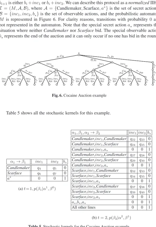
In this section we show the application of our approach to the Cocaine Auction
Pro-tocol [25]. The formalization of this proPro-tocol in terms of IIHSs using our framework
makes it possible to prove the claim in [25] suggesting that if the seller knows the iden-tity of the bidders then the (strong) anonymity guaranties are no longer assured.
Let us consider a scenario in which several mobsters are gathered around a table. An auction is about to be held in which one of them offers his next shipment of co-caine to the highest bidder. The seller describes the merchandise and proposes a starting price. The others then bid increasing amounts until there are no bids for 30 consecu-tive seconds. At that point the seller declares the auction closed and arranges a secret appointment with the winner to deliver the goods.
The basic protocol is fairly simple and is organized as a succession of rounds of bidding. Roundistarts with the seller announcing the bid pricebifor that round. Buyers havet seconds to make an offer (i.e. to say yes, meaning “I’m willing to buy at the current bid pricebi”). As soon as one buyer anonymously says yes, he becomes the winnerwiof that round and a new round begins. If nobody says anything fortseconds, round i is concluded by timeout and the auction is won by the winnerwi−1 of the previous round, if one exists. If the timeout occurs during round 0, this means that nobody made any offers at the initial priceb0, so there is no sale.
Although our framework allows the formalization of this protocol for an arbitrary number of bidders and bidding rounds, for illustration purposes we will consider the case of two bidders (Candlemaker and Scarface) and two rounds of bids. Furthermore, we assume that the initial bid is always1 dollar, so the first bid does not need to be announced by the seller. In each turn the seller can choose how much he wants to increase the current bid value. This is done by adding an increment to the last bid. There are two options of increments, namelyinc1(1 dollar) andinc2(2 dollars). In that way,
bi+1is eitherbi+inc1orbi+inc2. We can describe this protocol as a normalized IIHS
I = (M,A,B), whereA ={Candlemaker,Scarface, a∗}is the set of secret actions, B ={inc1, inc2, b∗}is the set of observable actions, and the probabilistic automaton
M is represented in Figure 6. For clarity reasons, transitions with probability0 are not represented in the automaton. Note that the special secret actiona∗ represents the
situation where neither Candlemaker nor Scarface bid. The special observable action b∗represents the end of the auction and it can only occur if no one has bid in the round.
Cm p1 Sfp2 a∗p3 inc1 q4 inc2q5 inc1 q6 inc2q7 b∗ 1 Cm p9 Sf p10 a∗p 11 p12Cm Sf p13 a∗p 14 p15CmSf p16 a∗p 17 p18Cm Sf p19 a∗p 20 a∗ 1 inc1 q22 inc2 q23 inc1 q24 inc2 q25 b1∗ inc1 q27 inc2 q28 inc1 q29 inc2 q30 b1∗ inc1 q32 inc2 q33 inc1 q34 inc2 q35 b1∗ inc1 q37 inc2 q38 inc1 q39 inc2 q40 b1∗ b1∗
Fig. 6. Cocaine Auction example
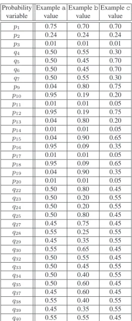
Table 5 shows all the stochastic kernels for this example.
α1→β1 inc1 inc2 b∗ Candlemaker q4 q5 0 Scarface q6 q7 0 a∗ 0 0 1 (a)t= 1, p(β1|α1, β0) α1, β1, α2 →β2 inc1 inc2 b∗
Candlemaker,inc1,Candlemaker q22 q23 0
Candlemaker,inc1,Scarface q24 q25 0
Candlemaker,inc1,a∗ 0 0 1
Candlemaker,inc2,Candlemaker q27 q28 0
Candlemaker,inc2,Scarface q29 q30 0
Candlemaker,inc2,a∗ 0 0 1
Scarface,inc1,Candlemaker q32 q33 0
Scarface,inc1,Scarface q34 q35 0
Scarface,inc1,a∗ 0 0 1
Scarface,inc2,Candlemaker q37 q38 0
Scarface,inc2,Scarface q39 q40 0
Scarface,inc2,a∗ 0 0 1
a∗,b∗,a∗ 0 0 1
All other lines 0 0 1
(b)t= 2, p(β2|α2, β1) Table 5. Stochastic kernels for the Cocaine Auction example.
The interested reader can find the construction of the reaction functions in Ap-pendix C.