Geometric numerical integration for optimisation

(1)

Geometric numerical integration for

optimisation

Erlend Skaldehaug Riis

Department of Applied Mathematics and Theoretical Physics

University of Cambridge

This dissertation is submitted for the degree of

Doctor of Philosophy

(2)

(3)

Declaration

This thesis is the result of my own work and includes nothing which is the outcome of work done in collaboration except as declared in the Preface and specified in the text. It is not substantially the same as any that I have submitted, or, is being concurrently submitted for a degree or diploma or other qualification at the University of Cambridge or any other University or similar institution except as declared in the Preface and specified in the text. I further state that no substantial part of my thesis has already been submitted, or, is being concurrently submitted for any such degree, diploma or other qualification at the University of Cambridge or any other University or similar institution except as declared in the Preface and specified in the text.

Erlend Skaldehaug Riis September 2019

(4)

(5)

Abstract

In this thesis, we study geometric numerical integration for the optimisation of various classes of functionals. Numerical integration and the study of systems of differential equations have received increased attention within the optimisation community in the last decade, as a means for devising new optimisation schemes as well as to improve our understanding of the dynamics of existing schemes. Discrete gradient methods from geometric numerical integra-tion preserve structures of first-order gradient systems, including the dissipative structure of schemes such as gradient flows, and thus yield iterative methods that are unconditionally dissipative, i.e. decrease the objective function value for all time steps.

We look at discrete gradient methods for optimisation in several settings. First, we provide a comprehensive study of discrete gradient methods for optimisation of continu-ously differentiable functions. In particular, we prove properties such as well-posedness of the discrete gradient update equation, convergence rates, convergence of the iterates, and propose methods for solving the discrete gradient update equation with superior stability and convergence rates. Furthermore, we present results from numerical experiments which support the theory.

Second, motivated by the existence of derivative-free discrete gradients, and seeking to solve nonsmooth optimisation problems and more generally black-box problems, including for parameter optimisation problems, we propose methods based on the Itoh–Abe discrete gradient method for solving nonconvex, nonsmooth optimisation problems with derivative-free methods. In this setting, we prove well-posedness of the method, and convergence guarantees within the nonsmooth, nonconvex Clarke subdifferential framework for locally Lipschitz continuous functions. The analysis is shown to hold in various settings, namely in the unconstrained and constrained setting, including epi-Lipschitzian constraints, and for stochastic and deterministic optimisation methods.

Building on the work of derivative-free discrete gradient methods and the concept of structure preservation in geometric numerical integration, we consider discrete gradient methods applied to other differential systems with dissipative structures. In particular, we study the inverse scale space flow, linked to the well-known Bregman methods, which are central to variational optimisation problems and regularisation methods for inverse problems.

(6)

In this setting, we propose and implement derivative-free schemes that exploit structures such as sparsity to achieve superior convergence rates in numerical experiments, and prove convergence guarantees for these methods in the nonsmooth, nonconvex setting. Furthermore, these schemes can be seen as generalisations of the Gauss-Seidel method and successive-over-relaxation.

Finally, we return to parameter optimisation problems, namely nonsmooth bilevel optimi-sation problems, and propose a framework to employ first-order methods for these problems, when the underlying variational optimisation problem admits a nonsmooth structure in the partial smoothness framework. In this setting, we prove piecewise differentiability of the parameter-dependent solution mapping, and study algorithmic differentiation approaches to evaluating the derivatives. Furthermore, we prove that the algorithmic derivatives converge to the implicit derivatives. Thus we demonstrate that, although some parameter tuning problems must inevitably be treated as black-box optimisation problems, for a large number of varia-tional problems one can exploit the structure of nonsmoothness to perform gradient-based bilevel optimisation.

(7)

(8)

(9)

Acknowledgements

After four years in Cambridge that have been beyond wonderful, and at the end of an occasionally chaotic PhD journey, there are many people I would like to thank for being in my life during this period, both in personal and professional capacities.

First of all, I am deeply grateful and indebted to my supervisor Carola Schönlieb. The thesis would not have happened without your academic guidance, support, generosity, and patience, and I count myself as exceptionally lucky to have had you as my doctoral supervisor, and to be a part of the Cambridge Image Analysis group.

I would sincerely like to thank everyone in the CIA by name, but fear at this point that the names alone would fill a page . However, I am very glad to have been in a research group in which academic and social isolation have been such alien concepts, and from which I have many fond memories. Matthias Ehrhardt, thank you for the enjoyable collaborations and discussions, as well as for encouraging me to apply for the LMS Early Career fellowship. Martin Benning, thank you for our collaboration, your guidance on how to ‘Bregmanise’ discrete gradient methods, and your positive energy. Tamara Großmann, thank you for our collaboration—amidst the ceaseless debugging of MATLAB toolboxes, it was great to work with you. Joana Grah, thank you for all the BBQs you hosted, and the lunches at Robinson. Finally, thank you Jingwei Liang for taking the time to talk through various aspects of partial smoothness with me.

My greatest thanks to Reinout Quispel and Robert McLachlan for the wonderful hospital-ity they showed me during my trips to Melbourne and Palmerston North. I am grateful for being introduced to geometric numerical integration during my stays with you. Furthermore, thank you to Reinout Quispel and Torbjørn Ringholm for our collaborations and discussions. Thanks as well to everyone in my cohort of the CCA, and an extra thanks to Eardi Lila for your former, involuntary role as my go-to MATLAB solver. I am grateful to Anders Hansen, for his time and guidance as my supervisor during the first year of CCA, and to Sarah Bohndiek and James Joseph for all the help and discussions during the project on photoacoustic tomography. Thank you to Andrew Stuart for all his support during my mas-ter’s studies, ultimately fooling CCA into accepting my application. Thank you to the CCA

(10)

directors for accepting me onto the programme. Finally, I am thankful to Cantab Capital Institute for the Mathematics of Information for funding the latter part of my PhD.

I sincerely thank the thesis examiners Prof. Elena Celledoni and Dr. Hamza Fawzi for carefully reading the manuscript and for the invaluable feedback and discussions during my viva.

Andria Pancrazi and Jenny Leivadarou, thank you for all the wonderful memories from my first year in Cambridge, and an extra shout-out to Jenny for her valiant efforts in convincing me to stick with the PhD. Thank you to Joel Mandella for visiting Cambridge twice, and of course the rest of the Mandellas, for all the times we have had together during the past 11 years. Thank you to my good friends Njål, Nicolai, and Grete for making the trip from Oslo. Last but not least, I would have not have completed this programme, let alone get into Cambridge, without the love and support of my parents through all the years, even in spite of all those slanderous stories I wrote in school about flawed parents. You make excellent parents, and promise I will take up Norwegian again some day. My sister Oda and brother Pål, at the risk of jinxing the end of my PhD, I look forward to demanding you call me ‘Dr Erlend’. My partner Freya, largely thanks to you, I have stayed relatively sane during the final weeks. Throughout my PhD, your ambition and academic abilities have inspired me to strive to work harder, which this thesis hopefully reflects.

(11)

List of figures

3.1 DG methods for linear systems with condition number κ =10 (left) and κ =1,000 (right). Convergence rate plotted as relative objective[F(xk)−

F∗]/[F(x0)−F∗]. Linear rate is observed for all methods and is sensitive to condition number. . . 57 3.2 Comparison of observed convergence rate with theoretical convergence

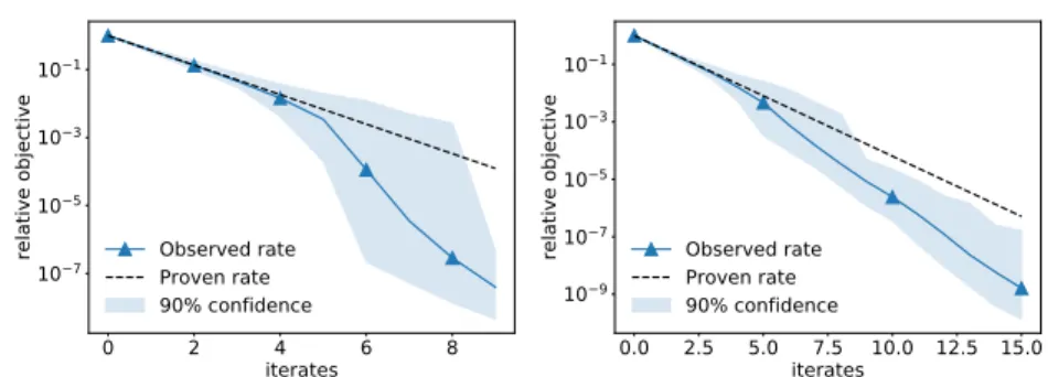
rate (3.24), for randomised Itoh–Abe method applied to linear system with condition numbersκ=1.2 (left) andκ =10 (right). Average convergence

rate and confidence intervals are estimated from 100 runs on the same linear system. The sharpness of the proven convergence rate is observed in both cases. . . 58 3.3 DG methods for linear systems with nontrivial kernel, and convergence

rate plotted as relative objective. Due to the kernel, the function is not strongly convex but nevertheless satisfies the PŁ inequality, hence the linear convergence rates. . . 58 3.4 CIA and RIA methods applied to linear system, with matrix entries created

from uniform distribution. CIA with the time step τ =1/[

√

nL](orange, circle)performs better than the same method with heuristic time stepτ=2/L

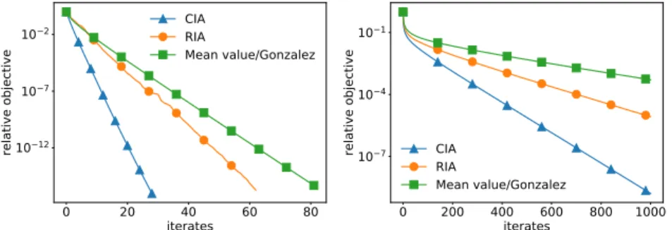
(blue, triangle), but worse than RIA. This is the reverse of what is observed if the matrix entries are created from Gaussian distribution. . . 59 3.5 DG methods forl₂-regularised logistic regression. Convergence rate plotted

as relative objective. The rates of randomised and cyclic Itoh–Abe methods almost coincide, and so do the mean value and Gonzalez discrete gradient methods. . . 60 3.6 DG methods applied to nonconvex problem that satisfies the PŁ

inequal-ity. Left: Plots of relative objective. Right: Plots of norm of gradient (normalised)∥∇F(xk)∥/∥∇F(x0)∥. . . 61

(16)

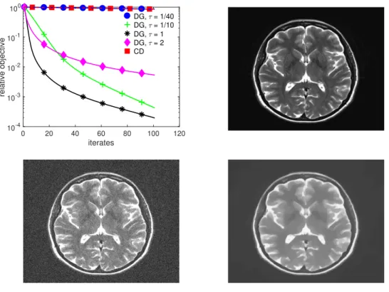
3.7 Top left: Comparison of explicit coordinate descent withτCD=1/(2λ √

ε+

1)vs the Itoh–Abe discrete gradient methods with time steps 0.025, 0.1, 1, and 2, and withε=10−8. Top right: Ground truth image. Bottom left: Noisy

image. Bottom right: Total variation denoising withε=10−8. . . 62

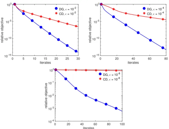
3.8 Comparison of CD to DG for three values ofε, 10−2, 10−4, and 10−8. The

time steps are set toτDG= √

τCDwhere the latter time step is set to 1/L. . . 63

3.9 Comparison of different time steps for CD vs fixed time step for DG. For smaller time steps, the CD iterates decrease too slowly, and for larger steps, they become unstable and fail to decrease. . . 64 3.10 Comparison of DG to simple backtracking line search (LS) in terms of

coordinate evaluations. . . 64 4.1 Comparison of three variants of the Itoh–Abe method applied to the

Rosen-brock function. Top left: Itoh–Abe method with standard frame. Top right: Rotated Itoh–Abe method. Bottom left: Itoh–Abe method with random pursuit. Bottom right: Convergence rates of the relative objective F(xk)−F∗

F(x0₎₋_F∗

for the three variants. . . 86 4.2 Comparison of three variants of the Itoh–Abe method applied to Nesterov’s

nonsmooth Chebyshev–Rosenbrock function. Top left: Itoh–Abe method with standard frame. Top right: Rotated Itoh–Abe. Bottom left: Itoh– Abe with random pursuit. Bottom right: Convergence rates of the relative objective F(xk)−F∗

F(x0₎₋_F∗ for the three variants. . . 87

4.3 Comparison of rotated Itoh–Abe method, LT-MADS and Py-BOBYQA applied to Nesterov’s nonsmooth Chebyshev–Rosenbrock function. Top left: The iterates from the Itoh–Abe method locate the unique minimiser to an order of accuracy of about 10−11. Top right: The iterates from the LT-MADS method locate the nonminimising stationary point. Bottom left: The iterates from the Py-BOBYQA method stagnate due to nonsmoothness. Bottom right: A plot of the relative objective F(xk)−F∗

F(x0₎₋_F∗ with respect to function evaluations,

(17)

List of figures xvii

4.4 Comparison of rotated Itoh–Abe method, LT-MADS and Py-BOBYQA applied to Nesterov’s nonsmooth Chebyshev–Rosenbrock function with a different starting point. Top left: The iterates from the Itoh–Abe method locate the unique minimiser to an order of accuracy of about 10−11. Top right: The iterates from the Py-BOBYQA method stagnate due to nonsmoothness. Bottom left: The iterates from the LT-MADS method locate the nonminimis-ing stationary point. Bottom right: A plot of the relative objective F(xk)−F∗

F(x0₎₋_F∗

with respect to function evaluations, for each method. . . 89 4.5 TV denoising reconstructions for different regularisation parameters. Top

left: Graph of F in (4.10). Top right: First parameter choice,ϑ1=10−2.

Bottom left: Second parameter choice, ϑ2=7×10−2. Bottom right: The

third parameter choice,ϑ3=2×10−1. . . 90

4.6 Wavelet denoising withL2scoring function and the Itoh–Abe method. Top left: Plot of iterates of the Itoh–Abe method. The rest: Image denoising results at different iteratesk. . . 93 4.7 Wavelet denoising with SSIM scoring function and the Itoh–Abe method.

Top left: Plot of iterates of the Itoh–Abe method. The rest: Image denoising result at different iteratesk. . . 94 4.8 TV denoising with SSIM scoring function and the Itoh–Abe method. Top

left: Plot of iterates of the Itoh–Abe method. The rest: Image denoising result at different iteratesk, with a zoom to show the difference. . . 95 4.9 TGV denoising with SSIM scoring function and the Itoh–Abe method. Top

left: Plot of iterates of the method. The rest: Image denoising result at different function evaluations j. . . 96 4.10 Comparison of optimisation methods for TGV denoising with SSIM scoring

function. Top left: Plot of iterates of the Itoh–Abe method. Top right: Plot of iterates of the LT-MADS method. Bottom left: Plot of iterates of the Py-BOBYQA method. Bottom right: Comparison of convergence rates for the methods with respect to function evaluations. . . 97 4.11 Comparison of optimisation methods for TGV denoising with SSIM scoring

function for a different starting point. Top left: Plot of iterates of the Itoh– Abe method. Top right: Plot of iterates of the LT-MADS method. Bottom left: Plot of iterates of the Py-BOBYQA method. Bottom right: Comparison of convergence rates for the methods with respect to function evaluations. . 98 5.1 Numerical results for the optimisation problem in (5.9), with iterates going

(18)

5.2 Numerical results for the optimisation problem in (5.10), with iterates going from red to black. . . 113 6.1 Comparison of SOR and sparse SOR methods, for Gaussian linear system

without noise. Left: Convergence rate for relative objective, i.e. [F(xk)− F∗]/[F(x0)−F∗]. Right: Support error with respect to iterates, i.e. propor-tion of indicesis.t. sgn(xk_i) =sgn(x∗_i). . . 127 6.2 Comparison of SOR and sparse SOR methods, for Gaussian linear system

without noise, and binary ground truth. Left: Convergence rate for relative objective. Right: Support error with respect to iterates. . . 127 6.3 Comparison of SOR and sparse SOR methods, for Gaussian linear system

with noise. Left: Convergence rate for relative objective. Right: Support error with respect to iterates. . . 128 6.4 Comparison of SOR and sparse SOR methods, for ℓ1-regularised linear

system with noise. Left: Convergence rate for relative objective. Right: Support error with respect to iterates. . . 128 7.1 The relative distance of the algorithmic derivative to the convex hull of local

derivatives with respect to iterates, i.e. dist(Dxk,∂x)/dist(Dx1,∂x). . . 166

7.2 Left: The relative objective of (7.35) with respect to the iterates, for FISTA and FB. Right: The relative error∥Dxk₍_ϑ₎₋_Dx₍_ϑ₎_∥_/_∥Dx1₍_ϑ₎₋_Dx₍_ϑ₎_∥

with respect to the iterate, for FISTA and FB, and implicit (Imp) and algo-rithmic (Alg) differentiation. . . 168 7.3 Left: The relative objective of (7.36) with respect to the iterates, for FISTA

and FB. Right: The relative error∥Dxk₍_ϑ₎₋_Dx₍_ϑ₎_∥_/_∥Dx1₍_ϑ₎₋_Dx₍_ϑ₎_∥

with respect to the iterate, for FISTA and FB, and implicit (Imp) and algo-rithmic (Alg) differentiation. . . 169 8.1 Discrete gradient methods applied to the optimisation problem (8.10). Left:

A comparison of the mean value discrete gradient method and the Itoh– Abe method. Right: A comparison of the two previous methods with the Bregman Itoh–Abe method. . . 179

(19)

List of tables

3.1 Estimates ofβ, as well as optimal time stepsτ∗and correspondingβ∗. Recall ζ is defined in (3.5). . . 49

3.2 Average CPU time (s) over 50 iterations of (2.8) with the mean value discrete gradient. Toleranceε=10−6. . . 65

(20)

(21)

Nomenclature

Differentials

Ck(_Rn;_Rm) The set ofktimes continuously differentiable functions f :_Rn→_Rm_.

C_ck(_Rn;Rm) The set of functions inCk(Rn;Rm)with compact support.

∇f Gradient of f :_Rn→_R.

D f The first-order differential of f.

∇xf(x,ϑ) Gradient with respect to spatial vectorx.

D_ϑ f(x,ϑ) Differential with respect to parametersϑ.

∇2f Hessian of f :Rn→R, i.e.∇2f = ∂ 2_f ∂xi∂xj ∂2f ∂xix2_j ! i,j=1,...,n .

f′(·;d) The directional derivative of f in the directiond. ∇x Discretised spatial gradient of the vectorx.

˙

x(t) The temporal derivative of a vector-valued functionx.

E Symmetrised gradient.

Functions

Γ0(Rn) The set of convex, proper, lower semicontinuous functions onRn.

gphf The graph of f.

domf The effective domain of f.

epif The epigraph{(x,α) : α ≥ f(x)}of f.

(22)

δ_Ω The indicator function ofΩ⊂_Rn. sgn(x) The sign function.

f◦g The composition of functions f andg.

f∗ The convex conjugate of f.

J_∨+_G _{The infimal convolution of}_J_and_G_.

Generalised differentials

∂f The (general) subdifferential of f. ∂Cf The Clarke subdifferential of f.

b

∂f The regular subdifferential of f. ∂∞f The horizon subdifferential of f.

fo(·;d) The Clarke directional derivative of f in the directiond.

D_f,Dsymm_f The Bregman distance and symmetric Bregman distance. ∇f A discrete gradient of f.

SGN(x) The (set-valued) subdifferential of|x|.

Linear algebra

A∗ The adjoint of a matrixA.

AH Hermitian adjoint of matrixA.

I_n Then×nidentity matrix. 0n Then×nzero matrix.

rank(A) Rank of matrixA.

σ(A) Spectrum of matrixA.

ρ(A) Spectral radius of matrixA.

κA The condition number of matrixA.

(23)

Nomenclature xxiii

kerA The kernel of a matrixA.

Miscellaneous

ei Theith coordinate vector of_Rn.

R

fds The integral of f with respect tos.

b( moda) The modulo operation.

Eξ The expectation with respect to distributionξ. f(x) =o(g(x)) Littleo: lim_∥_x_∥→₀∥f(x)∥/∥g(x)∥=0.

f(x) =O(g(x)) BigO: lim sup_∥_x_∥→₀∥f(x)∥/∥g(x)∥ ≤C<∞.

Numerical sets

N The set of natural numbers. Z The set of integers.

R The set of real numbers.

R The extended real numbersR∪ {±∞}.

R≥0 The set of nonnegative, real numbers.

C The set of complex numbers. Q The set of rational numbers. Rm,n The set ofm×nreal matrices.

Cm,n The set of complex-valuedm×nmatrices.

B_ε(x) The open ball of radiusε >0 atx.

B_ε(x) The closed ball of radiusε >0 aroundx.

Sn−1 The unit sphere in_Rn.

Norms

∥·∥,⟨·,·⟩ The Euclidean norm and associated inner product on_Rn.

(24)

∥·∥F The Frobenius norm for matrices.

|x| The absolute value ofx.

∥x∥1,2 The group lasso norm∑ni=1∥xi∥.

TV The total variation seminorm∥∇·∥1,2.

TGV The total generalised variation seminorm.

|x|γ The smoothed absolute value

p

x2+γ.

∥x∥_γ The smoothed normp∥x∥2₊_γ_.

∥x∥1,2,γ The smoothed group lasso norm∑ni=1∥xi∥γ.

TVγ The smoothed total variation seminorm∥∇·∥1,2,γ. Riemannian manifolds

TxM The tangent space of manifoldM.

N_xM The normal space of manifoldM. ∇Mf The Riemannian gradient of f alongM.

∇2_Mf The Riemannian Hessian of f alongM.

Wx The Weingarten map ofMatx.

Set operations

Xn Then-Cartesian product of a setX.

U _bV U is compactly contained inV.

X⊥ The orthogonal complement of a setX ⊂_Rn_.

[x,y] The line segment{λx+ (1−λ)y : λ ∈[0,1]}.

clΩ The closure ofΩ⊂_Rn. intΩ The interior ofΩ⊂_Rn.

bdΩ The topological boundary ofΩ, clΩ\intΩ. diamΩ The diameter ofΩ⊂Rn.

(25)

Nomenclature xxv

dist(Ω,x) The Euclidean distance fromx∈_Rn_to_Ω_⊂

Rn.

N_x Neighbourhood ofx∈_Rn_.

riΩ The relative interior ofΩ⊂_Rn.

rbdΩ The relative topological boundary ofΩ, clΩ\riΩ. coΩ The convex hull ofΩ⊂_Rn.

affΩ The affine hull ofΩ⊂_Rn. parΩ The subspace parallel to affΩ.

P_X The projection operator of a closed, convex setX⊂_Rn_.

TC

Ω The Clarke tangent cone ofΩ⊂R

n_.

TH

Ω The hypertangent cone ofΩ⊂R

n_.

Ω∞ The horizon cone ofΩ. b

N_Ω The regular normal space ofΩ.

N_Ω The (general) normal space ofΩ.

Abbreviations

ADMM Alternating direction method of multipliers BSOR Bregman successive-over-relaxation CCD Cyclic coordinate descent

CIA Cyclic Itoh–Abe method DG Discrete gradient

FISTA Fast iterative shrinkage-thresholding algorithm ISS Inverse scale space

KŁ Kurdyka–Łojasiewicz MADS Mesh adaptive direct search MRF Markov random field

(26)

MRI Magnetic resonance imaging ND Nondegeneracy

ODE Ordinary differential equation PDE Partial differential equation PDHG Primal-dual hybrid gradient PŁ Polyak–Łojasiewicz

RCD Randomised coordinate descent RIA Randomised Itoh–Abe method SOR Successive-over-relaxation SSIM Structural similarity index

(27)

Chapter 1 Introduction

In this thesis, we consider methods for solving various classes of optimisation problems, by combining tools from geometric numerical integration and nonsmooth optimality analysis. In this opening chapter, we provide the context and rationale for the research, and outline the contributions.

At the core of mathematical optimisation is the problem

min

x∈XF(x), i.e. findxthat minimisesF :X →R. (1.1)

This objective is notably simple. However, solving (1.1) can be arbitrarily difficult depending on the properties of the objective functionF, and whether or not such a problem is solvable will have implications for the feasibility of various scientific applications. Because of this, optimisation theory is a broad and dynamic field whose developments both influence and are influenced by advances in science and engineering.

In contemporary optimisation problems, one often encounters challenges such as high dimensionality ofX, nonsmoothness ofF, and nonlinearities inX and the gradient∇F. In part, this is due to the rise of big data and machine learning, as well as sophisticated sparsity and regularisation models in signal processing which invoke nonsmooth functions to promote efficient signal representations. This has lead to a surge of interest in first-order optimisation methods, which scale better than higher-order methods with respect to the dimension ofX, and which combine naturally with nonsmooth optimisation via proximal methods. While this has led to rapid developments of mathematical optimisation theory in recent decades, there is as much as ever a demand for the development of algorithmic frameworks in optimisation for handling complex, nonlinear dynamics in an efficient manner.

As is often the case in mathematics, a promising source of ideas and developments in optimisation is to start with perspectives and techniques from other areas of mathematics.

(28)

One such area which has played an integral role to optimisation in recent years is numerical integration. This is the study of numerical methods for solving systems of differential equations. The subfield geometric numerical integration is the systematic study of geometric structures of differential systems and structure-preserving numerical methods. A recurring theme of this thesis is how techniques from geometric numerical integration can be used to solve a wide range of optimisation problems, through the preservation of energy dissipation.

For the remainder of this chapter, we will provide brief introductions to first-order optimisation methods, variational optimisation problems from signal processing which motivate our research, and numerical integration applied to optimisation methods, and finally give an outline and summarise the contributions of this thesis in Sections 1.2 & 1.3

1.1 An overview of optimisation and numerical integration

1.1.1 First-order optimisation methods

The two most important building blocks to first-order optimisation methods areexplicitand

implicit gradient descent. For a differentiable functionF:_Rn→_R, starting pointx0∈_Rn_,

and strictly positive time steps(τk)k∈N, (explicit) gradient descent is given by

xk+1=xk−τk∇F(xk), (1.2)

while implicit gradient descent is given by

xk+1=xk−τk∇F(xk+1). (1.3)

As the names suggest, the former update is explicit, while the latter is implicit, i.e. one must solve (1.3) with respect toxk+1. Note that this is equivalent to

0=∇ F(xk+1) + 1 2τ_k∥x k₋_xk+1_∥2 .

It follows that ify7→F(y) +∥y−xk∥2/(2τk)is convex, thenxk+1solves (1.3) if and only if

it solves xk+1=arg min y∈Rn F(y) + 1 2τk ∥y−xk∥2. (1.4)

This mapping is called theproximal mappingofF atxk. Observe that this latter formulation gives us a notion of implicit gradient descent updates for nondifferentiable functions, provided the minimisation problem in (1.4) is computationally tractable. Of course, by itself this

(29)

1.1 An overview of optimisation and numerical integration 3

observation is not helpful, as solving (1.4) will in general be of similar difficulty as solving the problem (1.1), which in the end is what we are interested in. However, the formulation (1.4) is crucial for several reasons, some of which we will discuss now, and some which will be touched upon at different stages of the thesis.

We first emphasise that for nonsmooth variational optimisation problems, one is often able tosplitthe objective functionF:_Rn→_Rinto different terms, each of which is either continuously differentiable or admits computationally tractable updates for (1.4). From hereon, we refer to functions in the latter category assimple. A well-known example of a simple function is theℓ1-norm∥x∥1:=∑n_i=1|xi|, for which the update (1.4) corresponds to

thesoft shrinkageoperator

S(xk,τk):=sgn(xk)max{|xk| −τk,0}, (1.5)

where sgn is the sign operator,

sgn(x):=          1, ifx>0, 0, ifx=0, −1, ifx<0,

and sgn, max and their products are evaluated elementwise. Another example is that of indicator functions of convex, nonempty, closed setsC⊂_Rn_,

δC(x):=    0, ifx∈C, +∞, otherwise, (1.6)

for which (1.4) corresponds to theprojection mapping

P_C(xk):=arg min

y∈C

1 2∥y−x

k_∥2_.

Second, as can be inferred directly from the equation, the update (1.4) isunconditionally dissipativewith respect to the time stepτkin the sense thatF(xk+1)≤F(xk)for anyτk>0.

This is in contrast to explicit gradient descent, in which the time step must be restricted according to the first-order regularity ofF in order to ensure energy decrease.

We return to proximal mappings in Section 2.4. For further details on proximal mappings, we refer to a survey by Combettes & Pesquet [55] and a monograph by Parikh & Boyd [172].

(30)

We point out that implicit gradient descent is also known as theproximal point algorithm

[101, 189].

To further emphasise that the proximal mapping (1.4) exists within a powerful framework for nonsmooth optimisation, we conclude this section by pointing out that there are various first-order splitting algorithms available for solving nonsmooth variational problems, based on combinations of implicit and explicit gradient descent steps.

These include forward-backward (FB) type methods when F is the sum of a smooth function and a simple function [14, 57, 173, 85], and the Douglas–Rachford method [75, 79, 138] and the related alternating direction method of multipliers (ADMM) whenF consists of two simple functions [27, 93]. Finally, primal-dual hybrid gradient (PDHG) methods [50, 226] are used for optimisation problems involving terms that are neither smooth nor simple but can be transformed into so-called saddle-point problems, and for which each term is either smooth or simple (see Section 2.4).

We return to PDHG and FB methods in Chapter 7 and Chapter 8, when we consider them for solving the lower-level problem of a bilevel optimisation problem (to be defined in the following section).

For a general treatment of convex analysis and monotone operator theory, see [12].

1.1.2 Variational optimisation problems

In what follows, we summarise common variational optimisation problems encountered in signal and image processing, and more generally inverse problems.

An inverse problem seeks to recover a signalx∈_Rn_{from data} _fδ _∈

Rl, via a forward

modelG:_Rn→_Rl_{, i.e. such that}_x_solves

fδ ₌_G₍_x_{) +}

δ, (1.7)

whereδ represents noise in the data fδ.

Before we introduce variational regularisation models for solving inverse problems, we motivate their necessity with the concept ofill-posedness. An inverse problem is said to be

well-posedif it admits auniquesolutionx∗∈_Rn_{such that}_G₍_x∗_{) =} _fδ_{, and which is stable}

with respect to perturbations in the data fδ_{. Due to the presence of noise in the data, as well}

as other uncertainties, such as errors in the forward modelG, a direct inversion ofGmight lead to an inaccurate reconstruction. Furthermore,Gis often ill-conditioned, meaning that even small amounts of noise in the data can lead to significant artefacts in the reconstruction. For these reasons, many inverse problems are ill-posed.

(31)

When an inverse problem is ill-posed, one needs to formulate a reconstruction model that finds a good signal match for the data, i.e. x such that G(x) is close to fδ_{, while}

simultaneously ensuring that the reconstruction adequately accounts for the uncertainty and instability in the inverse problem.

One popular approach is to use variational regularisation models, wherein one solves the variational optimisation problem

arg min

x∈Rn

F(G(x),fδ_{) +}_R₍_x_,

ϑ). (1.8)

HereF:_Rl_×

Rlis adata fidelityterm which measures the discrepancy betweenG(x)and fδ,

one example beingF(x,y) =∥x−y∥2/2, andR(·,ϑ)aregularisation term, which promotes

known information about the true signal, such as smooth regions and sharp edges of images, or signal sparsity in some coordinate frame.

We mention some regularisersR(·,ϑ)commonly used in image and signal processing.

The aforementionedℓ1-norm weighted byϑ ∈_R≥0, i.e. ϑ∥ · ∥1forϑ ≥0, is a popular

choice for promoting sparsity. We elaborate on this in the next subsection. Thetotal variation(TV) seminorm [48] in_Rnis defined as

TV_ϑ(x):=ϑ∥∇x∥1,2, ϑ ≥0. (1.9)

Here∇∈_R2n,ndenotes thediscretised spatial gradient for vectors in_Rn, as defined in [47], and ∥ · ∥1,2 is thegroup Lasso norm, which forz∈Rn,m is defined as∥z∥1,2:=∑n_i₌₁∥zi∥, wherezidenotes theith row vector ofz. This is the discretised version of total variation. We introduce its original, continuous formulation in Section 4.5.2. This regulariser is popular in image processing for its ability to preserve edges while penalising noise [196].

In spite of the prevalence of the TV regulariser, one of its drawbacks is that it promotes piecewise constant features, which can lead to so-called staircasing effects when the input image has linear features. To remove noise while promoting linear and higher-order features in images, Bredies et al. proposed thetotal generalised variation(TGV) seminorm [29]. In the discretised setting, this is given by

TGV_ϑ₁,ϑ2(x):= min

v∈R2n,n

ϑ1∥∇x∥1,2+ϑ2∥Ev∥1,2, ϑ1≥0,ϑ2≥0, (1.10)

whereE is the symmetrised gradient [29]. Similarly as forTV, the continuous formulation is given in Section 4.5.2.

We emphasise that regularisers are often parametrised, and the reconstruction of (1.8) therefore depends on the parameter choiceϑ. A common practical and theoretical challenge

(32)

in solving inverse problems is to tune these parameters appropriately. This leads to the class ofbilevel problemswhich we will discuss later in this chapter, and which is a recurring topic in this thesis.

For a review of regularisation methods for inverse problems, see [18, 83].

Nonsmoothness in variational problems

A central topic in this thesis is nonsmoothness in optimisation problems. As can be observed in the previous subsection, nonsmoothness is also a common feature for variational regulari-sation models—e.g. the three aforementioned regularisers are nonsmooth. In what follows, we will further motivate why nonsmoothness plays an important role in signal processing, and why frameworks and methods that account for nonsmoothness in optimisation problems are worth pursuing.

We take the example of signal sparsity and compressed sensing [73]. Since the seminal works of Daubechies, Meyer, et al. on wavelets and compressibility [6, 64, 150, 151], it is well-known that real-world signals such as audio recordings and images are highly

compressiblein certain bases and dictionaries. Compressibility in this context means that in some basis, such as the wavelet basis, the signaly∈_Rm_{can to a high level of accuracy be}

represented by a small number of bases vectorssrelative to its ambient dimensionalitym, i.e. s≪m. Given a signaly∈_Rm_{and a dictionary matrix}_W _∈

Rm,nwhich can be seen as

a transformation from the sparsity basis to the basis ofy, it is therefore of interest to find a sparse vectorx∈_Rn_{such that}_{W x}_≈_y_{. A reasonable variational approach to this is to solve}

1

2∥W x−y∥

2₊

ϑ∥x∥0,

where∥x∥0=|supp(x)|is the number of nonzero elements inx, and supp(x):={i : xi̸=0}.

However, as∥·∥0is nonconvex and discontinuous, this problem is computationally intractable

[41]. Alternatively, one could solve the optimisation problem 1

2∥W x−y∥

2₊

ϑ∥x∥1.

In addition to being convex and continuous, recall that∥ · ∥1is simple, so this problem is

amenable to proximal splitting methods.

Compressibility of signals has proven to be a powerful idea, with several applications. In

compressed sensing[41, 73], one exploits the inherent redundancy of information in signals to allow for subsampling of fδ_{, i.e. only observe a subset of the elements of} _fδ_{, while still}

(33)

that these recovery guarantees hold if one replaces∥ · ∥0with the convex relaxation∥ · ∥1like

we did above [41, Theorem 1.3]. This has implications e.g. for magnetic resonance imaging (MRI), as it allows for a significant reduction in scanning time [143].

Another example where data compressibility has played a crucial role is in the domains of big data, where the mere scale of the data collected renders compression a practical necessity. This includes astronomy [117, 174, 217] and genomics [140].

These examples illustrate that nonsmooth functions play an integral role in modelling and exploiting structures of signals, for methods in signal processing.

Bilevel optimisation problems

To conclude this subsection, we introduce a class of optimisation problems in which there is another layer of complexity to account for. These arebilevel optimisation problems, in which one seeks to optimise the parameters that go into a variational regularisation problem. As mentioned earlier, it is common to parametrise regularisation terms, e.g. withϑ in (1.8),

yet choosing these parameters optimally can be difficult. A bilevel optimisation problem is given by

min

ϑ∈Ω

E(x_ϑ,ϑ) s.t. xϑ ∈arg min

x∈Rn

F(x,ϑ), _(1.11)

whereΩ⊂Rmis the parameter space,E:Rn×Ω→Ris anupper-level objective function

which takes as input the parameter choiceϑ as well as the corresponding signal reconstruction

x_ϑ, andF :_Rn×Ω→Ris alower-level objective function, e.g. as given in (1.8).

What makes bilevel problems particularly difficult to solve is that the mappingϑ 7→

arg min_xF(x,ϑ)might be set-valued if F(·,ϑ) is not strongly convex, nonsmooth if F is

nonsmooth, and the mappingϑ 7→E(xϑ,ϑ)is generally nonconvex due to the nonlinearity

of the solution mappingϑ 7→xϑ. Furthermore, computingxϑ for a single choice ofϑ can be

computationally costly, and computing derivativesD_ϑx_ϑ, when this is possible, even costlier. In summary, bilevel problems for nonsmooth variational regularisation problems are nonsmooth, nonconvex, and computationally expensive. In fact, bilevel problems are in general NP hard [70]. See [40] for a review of bilevel optimisation for image processing.

The combination of nonsmoothness and nonconvexity has proven to be particularly challenging in optimisation problems, in comparison to for example convex, nonsmooth problems, whose theory is fairly well understood (see Section 2.4). With the exception of cases where the objective function can be split into a convex term and a smooth term, there are relatively few methods available for solving nonsmooth, nonconvex optimisation problems.

(34)

Several of the methods studied in this thesis address this class of problems, and are motivated by solving bilevel problems. That is, in Chapters 4 & 5, we propose derivative-free methods for nonsmooth, nonconvex optimisation problems, with applications to bilevel optimisation, and in Chapter 7, we study generalised differentiability of the solution mapping

ϑ 7→x_ϑ for nonsmooth variational problems.

We conclude these sections by reemphasising that nonsmoothness is an essential aspect of signal processing and optimisation methods. Yet in different contexts of optimisation, they continue to pose challenges, and hence there is a need for new optimisation methods that address these challenges, as well as new approaches to formulating and studying optimisation schemes. Furthermore, while explicit gradient descent and proximal mappings are powerful tools for solving various optimisation problems, they may not be applicable in cases where gradients are not accessible or the nonsmooth functions are not simple. It is therefore of interest to look at optimisation schemes that are applicable in more general settings.

1.1.3 Numerical integration

Numerical integration is the study of numerical methods for solving systems of differential equations. In recent years, this field has received increasing attention from the mathematical optimisation community, due to the idea that optimisation schemes can be understood through their relation to continuous-time differential systems and the numerical integration methods that connect them. We illustrate this with some examples.

The relevance of numerical integration to optimisation should not be surprising, consider-ing that explicit and implicit gradient descent (1.2), (1.3), the two, main buildconsider-ing blocks of first-order optimisation methods can be viewed as the forward and backward Euler method [114] respectively applied to the differential system known as thegradient flow,

˙

x(t) =−∇F(x(t)), x(0) =x0∈Rn, t≥0. (1.12)

Furthermore, their stability properties, e.g. unconditional dissipativity of (1.3) with respect to the time stepτk, can be inferred from the properties of the Euler method.

A prominent example of the study of differential equations and numerical integration to address challenges in optimisation is that of understanding theacceleration phenomenon. In 1983, Nesterov introducedaccelerated gradient descent[157] as a method that matches the optimal convergence rate ofO(1/k2)for first-order methods onL-smooth, convex functions. Since the resurgence of first-order methods in the era of big data and high-dimensional optimisation, acceleration techniques have received significant attention in the past decade,

(35)

for solving problems such as compressed sensing [16], training of deep and recurrent neural networks [210], and sparse linear regression [14].

In spite of its prevalence, the underlying dynamics of acceleration schemes are not well-understood, prompting several recent approaches to identify a framework in which to understand these schemes, taking perspectives from numerical integration. Su et al. [208] and Wibisono et al. [219] identify second-order ordinary differential equations (ODEs) that can be seen as continuous-time limits of the acceleration schemes. In the former case, this enables them to explain the oscillatory behaviour of acceleration scheme by interpreting the ODEs as damping systems. In the latter case, they present a family of

Bregman Lagrangian functionalswhich generate the original and new acceleration schemes. Furthermore, they demonstrate that the choice of ODE discretisation method is crucial for whether the acceleration phenomena is retained in the iterative scheme.

Several works have contributed to this setting of numerical analysis of acceleration methods which bridges continous-time and discrete-time dynamics. Wilson et al. [220] approach this from the perspective of Lyapunov theory, presenting Lyapunov functions accounting for both continuous- and discrete-time dynamics. Betancourt et al. [23] present a framework ofsympletic optimisation, i.e. considering perspectives of Hamiltonian dynamics and symplectic structure-preserving methods.

In a similar vein, recent papers by Maddison et al. [144] and França et al. [92] have studied conformal Hamiltonian systems, with the former focusing on how information about the the objective function’s convex conjugate can be incorporated to obtain stronger convergence rates, and the latter on structure-preserving numerical methods and their relation to different iterative schemes.

Another central issue for iterative optimisation schemes is the choice of time stepτk,

which is closely tied to stability analysis of numerical methods. In this context, tools from numerical integration can be used to formulate iterative schemes that allow for the use of larger time steps and therefore faster progression towards the minimum. Eftekhari et al. [80] achieve this for strongly convex problems, by formulating explicit stabilised descent methods that use explicit Runge–Kutta methods to maximise the total length of time steps [1]. The theoretical analysis demonstrates robustness with respect to the objective function’s condition number, and in numerical examples the method is shown to outperform accelerated gradient descent.

Other numerical integration methods include implicit Runge-Kutta methods, where energy dissipation is ensured under mild time step restrictions [104]. Finally we mention that one may consider gradient flows under non-Euclidean metrics, such as Bregman distances (see Chapter 6) and the Wasserstein metric [5, 200] (see Section 8.3.1).

(36)

Geometric numerical integration

In this thesis, we are particularly interested in geometric structure-preserving methods, which is the domain of geometric numerical integration. As described by Iserles & Quispel in

‘Why Geometric Numerical Integration?’[115], differential equations may exhibit geometric invariants, such as conservation laws of Hamiltonian energies, or Lie point symmetries, each of which imply that the solution to the differential equations is restricted to some lower-dimensional manifold. One is then interested in numerical methods which preserve these structures in some sense.

We highlight one class of methods from geometric integration, namelydiscrete gradient methods[97, 116, 148, 183]. These are designed for differential equations that can be written inlinear-gradient-form, i.e.

˙

x(t) =A(x(t))∇F(x(t)), (1.13) whereAis a matrix-valued function. By applying the chain rule, we derive

dF(x(t))

dt =⟨∇F(x(t)),A(x(t))∇F(x(t))⟩,

from which one can observe that the system is conservative, i.e.F is constant alongx(t), ifA

isskew-symmetric, i.e. A∗=−A. Similarly, we observe that the system is dissipative ifA

is negative-definite i.e.−Ais positive-definite—see Section 2.3. In fact, [148, Proposition 2.1 & Proposition 2.8] show that conservative and dissipative systems can in general be expressed in linear-gradient form.

Discrete gradient methods preserve the geometric structures of linear-gradient systems, e.g. energy conservation and dissipation laws, as well as Lyapunov functions. Furthermore, the methods areunconditionally stable, in the sense that these properties are preserved for all discretisation time stepsτk>0. This has prompted the study of discrete gradient methods

applied to gradient flows for solving optimisation problems. We give some examples. Grimm et al. [100] propose using discrete gradient methods for solving variational regularisation problems in image analysis. The applications include image inpainting and denoising, and they prove that for continuously differentiable objective functions, the methods converge to a set of stationary points. Furthermore, they compare the stability properties with other methods, such as Euler methods. In a similar setting, Ringholm et al. [185] consider the

Itoh–Abediscrete gradient method for solving image inpainting problems regularised with Euler’s elastica. These are nonconvex optimisation problems whose gradients are expensive to compute, while the Itoh–Abe discrete gradient (defined in Section 2.7) is derivative-free.

(37)

1.2 Contributions 11

Their numerical results suggest that this method is competitive with state-of-art methods for nonconvex variational optimisation problems.

Going beyond gradient flows in Euclidean space, Celledoni et al. [44] extend the discrete gradient method to solve Riemannian gradient flow systems on manifolds. In this setting, they prove that the iterates of the method converge to a set of stationary points. They apply the method to solve eigenvalue problems, as well as imaging problems that can naturally be formulated on manifolds.

For some reviews of the field of geometric numerical integration, we refer the reader to [105, 115, 147].

In summary of this section, numerical integration has in recent years shown great promise in providing new perspectives and frameworks for addressing challenges in optimisation. As we detail in the next section, we are interested in various optimisation problems, including those concerning nonsmooth energies, and we are interested in the use of discrete gradient methods from geometric numerical integration applied in this setting.

1.2 Contributions

In what follows, we summarise the motivations for and contributions of each chapter.

Chapter 3: The foundations of discrete gradient methods for smooth

optimisation

This chapter is based on the preprint [81], which is joint work done in collaboration with Matthias J. Ehrhardt, Torbjørn Ringholm, and Carola-Bibiane Schönlieb. The purpose of this chapter is to provide a comprehensive analysis of discrete gradient methods for the optimisation of continuously differentiable functions. While these optimisation methods have already been applied in various contexts for variational regularisation problems [100, 185], linear systems [153], and preserving Lyapunov functions [108], various aspects of the theoretical analysis have until now been lacking.

In this chapter, we address several issues, including convergence rates of the methods, well-posedness of the discrete gradient equation (2.8), and how to solve (2.8) efficiently. In particular, in Theorem 3.4 we prove for the three main discrete gradient methods that the discrete gradient equation admits a solution for all time steps. Furthermore, we prove that the discrete gradient methods essentially inherit the convergence rates of explicit gradient descent, yieldingO(1/k)rates for convex functions, and linear rates for strongly convex functions. Meanwhile, we propose a novel scheme for solving the discrete gradient equation, which we

(38)

demonstrate to be theoretically and numerically superior in certain cases. Furthermore, we propose and study a natural generalisation of the Itoh–Abe discrete gradient method, akin to randomised coordinate descent and random pursuit methods. The theory is supported with numerical experiments.

Chapter 4: Discrete gradient methods for nonsmooth, nonconvex

opti-misation

This chapter is based on the preprint [184], which is joint work done in collaboration with Matthias J. Ehrhardt, G. R. W. Quispel, and Carola-Bibiane Schönlieb. In this chapter, we consider the Itoh–Abe discrete gradient method for solving nonsmooth, nonconvex optimisation problems. Since this discrete gradient is derivative-free, it provides us with a notion of gradient flow-type dissipation in a black-box setting where we only have access to function evaluations.

We consider theClarke subdifferentialframework [54], defined in Section 2.5, for locally Lipschitz continuous functions. In this setting, we prove for randomised extensions of the Itoh–Abe discrete gradient method, as well as deterministic variants, that the iterates converge to a limit set of Clarke stationary points. Convergence guarantees in the deterministic case is based on a property termedcyclical density. While the analysis in this chapter can be used for discrete gradient methods, they are immediately generalisable to other line search-based, derivative-free methods in the Clarke subdifferential setting, thus allowing for optimality analysis for a wider class of derivative-free optimisation algorithms. Noting that many bilevel problems are nonsmooth, nonconvex, and challenging to compute gradients for, we consider the proposed methods for solving these problems. Furthermore, we compare with state-of-art derivative-free optimisation algorithms, thereby demonstrating the competitiveness of the proposed methods.

Chapter 5: Discrete gradient methods for nonsmooth, nonconvex,

con-strained optimisation

In this chapter, we build on the analysis of the previous chapter for derivative-free optimisation of nonsmooth, nonconvex functions, by extending the algorithm and convergence analysis to constrained optimisation problems. The reason for this is that parameter-optimisation problems often involve constraints on the parameters, varying from explicit constraints to more complicated, implicitly defined constraints. We study this problem in a general setting, only assuming that the constraint is epi-Lipschitzian [188], which essentially means it is the

(39)

1.2 Contributions 13

level set of a locally Lipschitz continuous function. The Clarke subdifferential framework is extended to define stationary points constrained to a set, and in this framework, we prove that the algorithm converges to a set of stationary points.

Chapter 6: Bregman discrete gradient methods for sparse optimisation

This chapter is based on the article [20] published in the Journal of Mathematical Imaging and Vision, and which is joint work done in collaboration with Martin Benning and Carola-Bibiane Schönlieb. While in the previous chapters, we look at discrete gradient methods applied to gradient flows, in this chapter we consider discrete gradient methods applied to the inverse scale space flow [201], which is a dissipative differential system closely related to Bregman iterative methods. This system allows us to incorporate additional structure into the scheme, to promote sparsity or other features of the objective function and the ground truth. We study the Itoh–Abe discrete gradient method applied to this flow, and prove convergence in a nonsmooth, nonconvex subdifferential framework. We implement this method for different Bregman distances and objective functions, generalising well-known methods such as Gauss-Seidel and successive-over-relaxation (SOR) for sparse optimisation. Through numerical experiments, we observe that for sparse ground truths, the Bregman discrete gradient methods converge significantly faster than regular SOR. Furthermore, the analysis in this chapter opens the door for the application of discrete gradient methods to other, non-Euclidean gradient flows.

Chapter 7: Differentiation for nonsmooth bilevel optimisation

In this chapter, we focus exclusively on bilevel optimisation problems, seeking to exploit structured nonsmoothness of the corresponding variational problem to differentiate with respect to the parameters. To do so, we employ the framework of partial smoothness [130]. For a large class of bilevel problems, we demonstrate piecewise differentiability of the solution mapping in Theorem 7.29, allowing us to characterise the Clarke subdifferential of the bilevel objective function. Furthermore, we prove for various forward-backward type algorithms, including accelerated variants, that the algorithmic derivatives converge to the limiting, implicit derivative in Theorem 7.33.

(40)

1.3 Outline of chapters

Chapter 2: Mathematical preliminaries

In Chapter 2, we define notation and basic mathematical tools used throughout the thesis. Specifically, we provide background material for linear algebra, convex and nonconvex optimality analysis, tools for first-order optimisation methods, and finally discrete gradient methods and geometric numerical integration.

Chapter 3: The foundations of discrete gradient methods for smooth

optimisation

After the introduction, we present a new existence result for the discrete gradient equation, based on the Brouwer fixed point theorem in Section 3.3. In Section 3.4 we study fixed point iterative methods for solving the discrete gradient equation, including a relaxed fixed point method with improved efficiency, while in Section 3.5, we study the dependence of the updatexk+1←_[xk on the time stepτk>0 for the mean value discrete gradient and the

Itoh–Abe methods. In Sections 3.6 and 3.7, we prove convergence rates for the discrete gradient methods, and convergence guarantees for functions that satisfy the strong Kurdyka– Łojasiewicz inequality, respectively. Before a brief discussion of preconditioned methods in Section 3.8, we present numerical results in Section 3.9.

Chapter 4: Discrete gradient methods for nonsmooth, nonconvex

opti-misation

In Section 4.1, we discuss the background for nonsmooth, nonconvex optimisation, and the purpose of the chapter. In Section 4.2 we provide the main theoretical results of the chapter, namely that the generalised Itoh–Abe methods converge to a connected set of Clarke stationary points. In Section 4.4 we propose an algorithm for solving black-box optimisation problems, and in Section 4.5 we provide numerical examples.

Chapter 5: Discrete gradient methods for nonsmooth, nonconvex,

con-strained optimisation

In Section 5.1 we propose a modification of the Itoh–Abe methods for constrained problems and discuss related works, while in Section 5.2 we provide preliminary results on epi-Lipschitzian sets and Clarke subdifferential analysis in the constrained setting. In Section 5.3

(41)

1.3 Outline of chapters 15

we study the proposed optimisation algorithm and prove that the methods converge to a connected set of Clarke stationary points in the constrained setting as well. In Section 5.4 we present numerical results.

Chapter 6: Bregman discrete gradient methods for sparse optimisation

After introducing the inverse scale space flow in Section 6.1, we propose to solve it using a Bregman discrete gradient method based on the ISS flow in Section 6.2. In Section 6.3 we prove well-posedness and convergence results for this method in a nonconvex, nons-mooth framework. Furthermore, in Sections 6.4 and 6.5, we discuss particular examples of Bregman discrete gradient methods and prove equivalencies between methods derived from different numerical integration schemes, respectively, before providing numerical results in Section 6.6.

Chapter 7: Differentiation for nonsmooth bilevel optimisation

In Section 7.1 we discuss bilevel optimisation of nonsmooth variational problems and motivations for studying the differential properties of the solution mapping. In Section 7.2, we review examples of nonsmooth bilevel problems and existing approaches for solving them in literature. In Section 7.3 we provide preliminary concepts for the subdifferential analysis, and prove for a sufficiently general class of variational problems that they are subdifferentially regular. In Section 7.4 we define partly smooth functions, and show under reasonable assumptions that the solution mapping is piecewise differentiable. In Section 7.5 we study algorithmic differentiation of various first-order methods for solving nonsmooth variational methods, and prove convergence guarantees to the implicit derivative. In Section 7.6 we present some numerical results, and in Section 7.7 we conclude.

Chapter 8: Conclusion & outlook

In Sections 8.1 and 8.2 we summarise and discuss the results of this thesis. In Section 8.3 we discuss future directions of research building on the work in this thesis. In particular, in Section 8.3.1, we consider solving the Wasserstein gradient flow with discrete gradients. In Section 8.3.2, we propose the use of mean value discrete gradient methods for nonsmooth objective functions, under assumptions of partial smoothness. In Section 8.3.3, we discuss future work for gradient-based approaches to bilevel problems, considering algorithmic differentiation of primal-dual methods, and studying stability of algorithmic differentiation methods when the number of iterations is determined by a stopping rule.

(42)

(43)

Chapter 2 Mathematical preliminaries

In this section, we provide mathematical preliminaries which will be used throughout the thesis. We first consider basic properties of differentiable functions, followed by theory of the class of convex, proper, lower semicontinuous functions. Next we provide an overview of nonconvex generalised differential theory, which in comparison to its convex counterpart is rather less unified. We conclude with an overview of geometric numerical integration and in particular discrete gradients.

2.1 Basic notation and conventions

In a Euclidean space setting, we denote by ∥ · ∥and ⟨·,·⟩ the norm and associated inner product. Forx∈_Rn_and _p_>_{0, the}_ℓp_-norm_{∥ · ∥}

pis defined as

∥x∥p:= p

q

x₁p+x₂p+. . .+x_np, while∥x∥_∞:=maxi=1,...,n|xi|, and∥x∥0:=|supp(x)|.

We denote by(ei)n_i₌₁the standard coordinate vectors inRn. We denote by[x,y]the line

segment between two pointsx,y∈_Rn_i.e.

[x,y]:=λx+ (1−λ)y : λ ∈[0,1] .

Forε>0,x∈_Rn, we denote byBε(x)theopen ball of radiusε at x,{y∈Rn : ∥x−y∥<ε},

and byB_ε(x)theclosed ball of radiusε at x,{y∈_Rn : ∥x−y∥ ≤ε}. We denote bySn−1

(44)

We summarisebigandsmall o-notation. For two functions f :_Rn→_Rm_and_g_:

Rn→Rl,

if∥f(x)∥/∥g(x)∥ →0 as∥x∥ →0, then f(x) =o(g(x)). If there isε>0 andC>0 such that

∥x∥<ε implies∥f(x)∥ ≤C∥g(x)∥, then f(x) =O(g(x)). Similarly, suppose(xn)_k_∈_N⊂_Rn_and₍_yn₎

k∈N⊂Rmare two sequences. If∥xk∥/∥yk∥ →0

ask→∞, thenxk=o(yk), while if there isC>0 andK∈_Nsuch that∥xk_{∥ ≤}_C∥yk_∥_{for all}

k≥K, thenxk=O(yk).

2.2 Notation and results for functions

First we introduce some notation for differentiable functions. Fork∈_N, the set ofk-times continuously differentiable functions f :_Rn→_Rm_{is denoted by}_Ck₍

Rn;Rn), andCk(Rn)

for short whenm=1. For f ∈C1(_Rn;Rm), we denote by ∇f(x)its gradient atx, and for

f ∈C2(_Rn), we denote by∇2f(x)its Hessian atx. Furthermore, for parametrised functions

f(x,ϑ)we useDinstead of∇to denote differentiation with respect to the parametersϑ, and

we write∇xf(x,ϑ)andDϑf(x,ϑ)to denote differentiation with respect to first and second

argument respectively.

We say that a function f onRnisset-valued inRmif for eachx∈Rn, f(x)is a subset

ofRm, and we write f :Rn⇒Rm. An important example of a set-valued function is the

subdifferential given in Section 2.4.

Definition 2.1(Graph). For a function f :_Rn_⇒_Rm, itsgraphis the subset of_Rn×_Rm_given

by

gphf :={(x,v)∈_Rn×_Rm : v∈ f(x)}.

For single-valued functions, the graph is defined analogously.

Definition 2.2(Support). For a function f :_Rn→_Rm_{, its support is the set of points for}

which the function does not vanish, i.e.

suppf :={x∈_Rn _: _f₍_x₎_̸₌₀_}_.

We also state the implicit function theorem, which we will apply to study properties of discrete gradient equations in Chapter 3, as well as for computing gradients for bilevel problems in Chapter 7.

Proposition 2.3(Implicit function theorem [22, Proposition A.25]). Let f :_Rn×_Rm_→

Rnbe

a function such that for some(x∗,y∗)∈_Rn_×

Rm, f(x∗,y∗) =0, f is locally C1-smooth around

Geometric numerical integration for optimisation