Offline and Online Density Estimation for Large High-Dimensional Data

(1)

Michigan Technological University Michigan Technological University

Digital Commons @ Michigan Tech

Dissertations, Master's Theses and Master's Reports

2018

Offline and Online Density Estimation for Large High-Dimensional

Data

Aref Majdara

Michigan Technological University, [email protected]

Recommended Citation Recommended Citation

Majdara, Aref, "Offline and Online Density Estimation for Large High-Dimensional Data", Open Access Dissertation, Michigan Technological University, 2018.

(2)

OFFLINE AND ONLINE DENSITY ESTIMATION FOR LARGE HIGH-DIMENSIONAL DATA

By Aref Majdara

A DISSERTATION

Submitted in partial fulfillment of the requirements for the degree of DOCTOR OF PHILOSOPHY

In Electrical Engineering

MICHIGAN TECHNOLOGICAL UNIVERSITY 2018

(3)

(4)

This dissertation has been approved in partial fulfillment of the requirements for the Degree of DOCTOR OF PHILOSOPHY in Electrical Engineering.

Department of Electrical and Computer Engineering

Dissertation Advisor: Dr. Saeid Nooshabadi

Committee Member: Dr. Daniel Fuhrmann

Committee Member: Dr. Timothy Havens

Committee Member: Dr. Yeonwoo Rho

(5)

(6)

Dedication

To my dear mother Raziyeh and my loving father Iraj,

(7)

(8)

List of Figures

2.1 Example of mid-point binary partitioning scheme in 2D sample space. 14 2.2 Calculating four new cut probabilities at each level, in 2D space. . . 16 2.3 Sample data (N = 20,000) from a trimodal bivariate normal

distribu-tion. . . 19 2.4 Actual joint density of the data in Figure 2.3. . . 19 2.5 BSP cuts on the sample space of Figure 2.3, with N = 20,000 and

M = 200. The number of BSP cuts is 182. . . 20 2.6 Estimated marginal PDF and CDF, using copula transform, for N =

20,000 and M = 200. . . 24 2.7 Distribution of the transformed random variables F1(X1) and F2(X2),

with N = 20,000. . . 24 2.8 BSP cuts on copula-transformed sample space with N = 20,000 and

M = 200. The number of BSP cuts is 87. . . 25 2.9 Estimated joint density, using copula transform with N = 20,000 and

(13)

2.10 Partition scores with N = 20,000 and M = 200 sample partitions for

examples for (a) marginals in Figure 2.6, (b) copula in Figure 2.8. . 29

2.11 Flowchart for Bayesian sequential partitioning. . . 32

2.12 Flowchart for density estimation using copula transform. . . 33

2.13 Data structure extended, to store distribution of the data points in subregions. . . 41

2.14 Optimized data structure for storing distribution of data points in sub-regions for (a) copula-transformed estimation where intermediate data structure dataDist stores the indices todata, and (b) for each of the marginals, where the intermediate step is not required. . . 42

2.15 Execution time and KLD vs. sample size (N) for different values ofM for a 64-D dataset. . . 44

2.16 Clustering a 2D example. . . 62

(a) Original unlabeled data . . . 62

(b) Clustering decision graph . . . 62

2.17 Clustered data . . . 62

2.18 Execution time vs. sample size N. . . 63

(a) Density estimation time . . . 63

(b) Total clustering time . . . 63

(14)

2.21 Clustering a 2D example. . . 67 (a) Decision Graph . . . 67 (b) Clustered data . . . 67

3.1 Equalizing the marginal sample spaces for all blocksb = 1,2, ..., B. For each block b with the total number of tb subregions, the first and last

subregion volumesV₁b and V_tb

b are properly extended toV

0b

1 and Vt0bb. 80

3.2 KL divergence (KLD) for various block sizes . . . 83 3.3 Computation times for individual blocks, for various block sizes. The

standard deviations are reported on top of the plots. . . 85 3.4 Relation between computation time and the required memory, and the

block size for a high dimensional dataset with simple structure . . . 86 3.5 Memory requirements for storing output density information for

in-dividual blocks, for various block sizes. The standard deviations are reported on top of the plots. . . 87 3.6 Time to reach different target KLD values. The corresponding

parti-tion scores are reported in the legend. . . 88 3.7 Memory requirement for storing the processed output density

infor-mation for different target KLD values. The corresponding partition scores are reported in the legend. . . 89 3.8 Overall memory requirement (input data-block and output density

(15)

3.9 KLD and normalized partition score overN (PSN) versus sample space size . . . 92

3.10 Linear relationship between partition score over N (PSN) and KLD 93

3.11 Differential normalized partition scores overN (dPSN) versus the data-block size . . . 94

3.12 Time to reach target dPSN = 0.025, for various block sizes. The number of blocks to achieve the required dPSN and the achieved KLD values with respect to a block size of 80k are marked on the plot. . 98

3.13 Memory requirements for dPSN=0.025, for a complex high dimensional dataset. . . 99

3.14 Relationship between the computation time and the required memory, and the block size for a complex high dimensional dataset. . . 100

3.15 Relation between arrival rate, processing rate and change rate, with response time τresp and settling time τsett, (a) Rp ≥ Ra and _R1_c <

Bα L Ra + L Rp (b) Rp ≥Raand 1 Rc ≥ Bα L Ra+ L Rp (c) Rp < Ra and 1 Rc < Bα L Ra + L Rp (d) Rp < Ra and _R1_c ≥ Bα L Ra + L Rp . . . 104

3.16 Variations in KLD, in density estimation over a 64-dimensional data stream. . . 111

(16)

3.18 Variations in KLD, in density estimation over a 90-dimensional real data stream. . . 113

4.1 Density estimation error vs. N, for a range of block sizes. . . 118 4.2 Comparison of methods in terms of KLD vs. N, for various block sizes

(64-D data). . . 125 4.3 Comparing the methods of regular and progressive block averaging,

regarding computation time per block of data, for various block sizes. 126 4.4 Comparing the methods of regular and progressive block averaging,

regarding the number of binary cuts per block of data, for various block sizes. . . 127 4.5 Comparison of estimation error, for various block sizes, for a stream of

64-D data. . . 131 4.6 Comparison of Hellinger distance, for various block sizes, for a stream

(17)

(18)

List of Tables

2.1 BSP with direct and copula-transformed cuts on D-dimensional space for various dimensions, forN = 20,000, M = 200. . . 23 2.2 BSP with copula-transformed cuts on D-dimensional space, for three

different options. . . 26 2.3 List of main data structures used in copula-based implementation of

the BSP algorithm. . . 37 2.4 Impact of correlation on computation time and estimation accuracy

(N = 100,000, D= 64). . . 47 2.5 Speedup rates for parallelization over d and m, on a 4-core machine

(N = 100,000, D= 64). . . 50 2.6 Comparison of density estimations using the methods of BSP, KDE

and median-based cuts for the marginals (D= 64). . . 53 2.7 Comparison of density estimations using the methods of BSP, KDE

and median-based cuts, for the marginals for a bimodal skewed Beta distribution (D= 64). . . 56 2.8 Classification rates for some sample datasets . . . 59

(19)

(20)

Preface

This doctoral dissertation contains material previously reviewed and published or material submitted to scientific journals and conferences, currently under review. Full citation of these publications are as follows:

Chapter 2:

• Aref Majdara and Saeid Nooshabadi, Nonparametric density estimation using copula transform, Bayesian sequential partitioning and diffusion-based kernel estimator, Paper under review, IEEE Transactions on Pattern Analysis and Machine Intelligence.

• Aref Majdara and Saeid Nooshabadi, Efficient density estimation for high-dimensional data, Paper under review, IEEE Transactions on Knowledge and Data Engineering.

• Aref Majdara and Saeid Nooshabadi, Efficient data structures for density estimation for high-dimensional Big data structures, 2017 IEEE International Symposium on Circuits and Systems (ISCAS), Baltimore, MD, 2017, pp. 1-4.

(21)

Chapter 3:

• Aref Majdara and Saeid Nooshabadi, Block-wise density estimation over high-dimensional data streams, Paper under review, ACM Transactions on Knowl-edge Discovery from Data.

Chapter 4:

• Aref Majdara and Saeid Nooshabadi, Progressive update of binary partitions for efficient offline and online density estimation, Paper under review, IEEE Transactions on Knowledge and Data Engineering.

(22)

Acknowledgments

I would like to thank all those who have helped me learn. Very special thanks to my advisor, Dr. Saeid Nooshabadi for his support and patience throughout my PhD research. I would also like to thank Dr. Daniel Fuhrmann, ECE Department Chair, for the financial support through TA and RA positions. Many thanks to MTU Graduate School for providing financial support for my last semester, through Doctoral Finishing Fellowship.

I would like to thank my wonderful family: my dearest mother Raziyeh, my loving father Iraj, my dear brothers Adel and Abed, my lovely sister Atefeh, my wonderful sister-in-law Neda, and my dear brother-in-law Moahammad, for always giving me their undivided love and support, even from far far away. I would also like to include the youngest member of our family, my sweet and lovely nephew, Behrad, who brought joy and love to our lives. I love you all!

Many thanks to my PhD defense committee members, Dr. Daniel Fuhrmann and Dr. Timothy Havens from Department of Electrical and Computer Engineering, and Dr. Yeonwoo Rho from Department of Mathematical Sciences.

At the end, I would like to thank my dear friend Hossein Tavakoli, for being such a great friend and wonderful roommate during these years.

(23)

(24)

List of Abbreviations

BBSP Blockized Bayesian Sequential Partitioning BP Binary Partitioning

BSP Bayesian Sequential Partitioning CDF Cumulative Distribution Function CPU Central Processing Unit

DPSN Differential Partition Score Normalized GPU Graphical Processing Unit

KDE Kernel Density Estimation KL Kullback-Leibler

KLD Kullback-Leibler Divergence KNN K-Nearest Neighbors

LDA Linear Discriminant Analysis MAP Maximum a-posteriori Probability MPI Message Passing Interface

PCA Principal Component Analysis PDF Probability Density Function PMF Probability Mass Function PSN Partition Score Normalized

(25)

SIS Sequential Importance Sampling TPW Tiled Parzen Window

(26)

Abstract

Density estimation has wide applications in machine learning and data analysis tech-niques including clustering, classification, multimodality analysis, bump hunting and anomaly detection. In high-dimensional space, sparsity of data in local neighborhood makes many of parametric and nonparametric density estimation methods mostly inefficient.

This work presents development of computationally efficient algorithms for high-dimensional density estimation, based on Bayesian sequential partitioning (BSP). Copula transform is used to separate the estimation of marginal and joint densities, with the purpose of reducing the computational complexity and estimation error. Us-ing this separation, a parallel implementation of the density estimation algorithm on a 4-core CPU is presented. Also, some example applications of the high-dimensional density estimation in density-based classification and clustering are presented. Another challenge in the area of density estimation rises in dealing with online sources of data, where data is arriving over an open-ended and non-stationary stream. This calls for efficient algorithms for online density estimation. An online density estimator needs to be capable of providing up-to-date estimates of the density, bound to the available computing resources and requirements of the application. In response to this, BBSP method for online density estimation is introduced. It works based on collecting and processing the data in blocks of fixed size, followed by a

(27)

weighted averaging over block-wise estimates of the density. Proper choice of block size is discussed via simulations for streams of synthetic and real datasets.

Further, with the purpose of efficiency improvement in offline and online density estimation, progressive update of the binary partitions in BBSP is proposed, which as simulation results show, leads into improved accuracy as well as speed-up, for various block sizes.

(28)

Chapter 1 Introduction

1.1 Motivation

A variety of modern real-world applications including sensing technologies, security, financial trading, epidemiology, networks and scientific experiments, strongly rely on a proper and timely analysis of stationary or non-stationary streams of data [1] [2]. Density estimation can provide an effective way of obtaining useful insights on im-portant features of the data, such as multimodality and skewness [3]. While density estimation can be used for both continuous and discrete data, it is specially helpful in smoothing continuous data. It can be used as the basis of a range of statisti-cal analyses and machine learning techniques, including non-parametric discriminant

(29)

analysis [4], classification, feature analysis [5], cluster analysis [6], bump hunting [7], and anomaly detection [8]. Statistical analysis of big data typically requires analytics in high-dimensional domain, where many of the commonly used techniques fail to perform [9].

Furthermore, with growing availability of data in large volumes, development of com-putationally efficient data analysis algorithms has become of great importance, in various fields of science and technology. This efficiency can be stated in terms of a number of parameters, including computation time and memory requirements. In applications with data continuously arriving over a stream, analysis of the data needs to be performed in an online fashion, i.e. the data needs to be processed as it arrives. Efficiency in terms of computation time becomes critical in these online applications. If the rate at which the data is being processed is lower than the arrival rate of data, the processing system will not be able to provide up-to-date results. This work studies the problem of density estimation in high dimensions, with a focus on developing computationally efficient data structures and algorithms, for offline and online applications.

1.2 Background

(30)

visualiz-[13], bioprocessing [14], etc.

Multivariate density estimation serves as the basis for many of data mining and ma-chine learning techniques. Density estimation is defined as the process of constructing an estimate of the probability density function (PDF), from a set of observed data. For a D-dimensional random vector X = (X1,· · · , XD), its PDF fX(x), where the

vector x= (x1,x2,· · · ,xD), can be used in computing the probability that point X

is located in a certain D-dimensional domain D= (D1,D2,· · · ,DD), is defined as,

P(X ∈D) =

Z

D

fX(x)dx (1.1)

where dx= dx1dx2· · ·dxD.

Typical parametric density estimation methods [3] [15] [16] assume that the data is coming from a known type of distribution,e.g. Normal distribution with meanµand

variance σ2. Then the process of density estimation aims at estimating the values of theses parameters. However, in high-dimensional problems, parametric methods become largely inefficient, as due to sparsity of data in some areas of the sample space, the number of parameters rapidly increases with the sample size and dimension (a.k.a.

curse of dimensionality)[15] [17] [18].

Non-parametric methods are more suited for high-dimensional data, as they do not assume any characteristic structure for the data. In these methods, the number of parameters is not fixed, which makes them more flexible than parametric methods.

(31)

Kernel density estimation (KDE) [3] [15] [16] [19] [20] [21] is one of the most popular non-parametric density estimators, and is defined by [3],

ˆ f(x) = 1 N hD N X i=1 K x−Xi h (1.2)

where K is the kernel function, Xi represents the ith sample and h is called the

bandwidth. In kernel methods, proper choice of the bandwidth is critical, specially in

high-dimensional problems.

The most commonly used data-driven method for bandwidth selection is the plug-in

method [22] [23]. However, this method is found to be negatively affected by the normal reference rule [24] [25] [26].

The work in [26] introduces an adaptive method for kernel density estimation, based on linear diffusion processes and their smoothing properties. They view the kernel of the estimator as the transition density of a diffusion process. In addition, to avoid the negative effects of the normal reference rule, they introduce an improved method for calculating the plug-in bandwidth. Their new nonparametric plug-in method does not require assuming a preliminary Normal model. Main part of their work focuses on one-dimensional problems, but they claim that their method can be extended to higher dimensions.

Some work has been done on density estimation methods using decision trees [27]. In these tree-based methods, the density estimation process involves learning a set of

(32)

rules, which are then used for estimating the density for each given test point. In [27], they have presented examples of density estimation for up to 784 dimensions, as well as density-based binary and multi-class classification examples for a 64-dimensional classification problem.

Methods for nonparametric density estimation using wavelets are discussed in [28]. Other works in density estimation include use of weak classifier for density estimation [29] and density estimation based on nearest and farthest neighbor [30].

Multivariate kernel methods [31] [32] are frequently used for multivariate density estimation. The work in [31] presents simulation results for up to 5-dimensional examples. RS-Forest method proposed by [8] provides a fast density estimator for anomaly detection over streams. It uses a forest of randomized space trees (RS-Trees) to partition the data space. In [33], nonparametric multivariate density estimation is performed based on the integration of several multivariate histograms.

In some applications like change point detection in time series [34], estimation of density differences is desired. Some work has been done on direct estimation of density differences [35] [36], and density ratios [37] [38]. Some other works [39] have used an extension of the P´olya Tree [40] to develop a framework for multivariate density estimation. The high computational complexity of this method makes it not a good choice for high-dimensional problems.

(33)

Another non-parametric density estimation method is thehistogram with fixed

multi-dimensional bin volume, which is widely used in univariate problems for obtaining a quick estimate of the density function. The basic idea of the histogram can be easily extended to higher dimensions. A multivariate histogram works based on the simple idea of dividing the sample space into equal multi-dimensionalbins of volumehD _and

then counting the number of data points in each bin, to obtain a piecewise constant estimate of the underlying density function. However, with equally spaced bins, it is not possible to adapt to spatially varying smoothness [41]. Even more significantly, in multivariate space, the density function may vary unevenly across the dimensions. To deal with this, various histogram methods with adaptive choice of the bin volume have been proposed [41] [42]. For a variable bin volume histogram with fixed bin size projected along each dimension, the bin volume can be expressed ash =h1h2· · ·hD.

For a more general case of variable bin sizes along each dimension, a D-dimensional bin volume can be expressed as hj=(j1,···,jD) =

QD

d=1hjd, with 1 ≤ jd ≤ jdmax. In

general hjd 6= hkd, or more generally hj 6= hk. For a sample X =x, located in the D-dimensional bin volume of hj, the density is estimated as [3],

f(x) = 1

N ×

nj hj

(1.3)

where N is the total number of samples and nj is the data count in bin volume hj.

Even with variable bin sizes, the direct application of histogram with regular grid structure becomes impractical as the number of bins required grows exponentially

(34)

with the dimension. As an example, for a 10-dimensional test case in MATLAB®, the maximum number of bins that can be allocated before the system runs out of memory is 810. This corresponds to only eight bin segments along each dimension! To significantly reduce the number of bins, requires partitioning the sample space into irregular partitions of various sizes. The method of adaptive histogram, in which the irregular bin volumes are chosen in a data-dependent way, has been proposed before [41] [42] [43] [44] [45]. Data-dependentBayesian sequential partitioning (BSP)

method using sequential importance sampling (SIS) [46] [47] has been proposed [9] as an efficient way of partitioning the sample space, based on Bayesian inference. Binary partitioning of the sample space in a sequential fashion, has also been used in [48], for creating a data-adaptive partition over the sample space. Star discrepancy [49] is used as a measure of uniformity of data distribution, in order to decide which areas of the sample space need further partitioning.

In this dissertation, BSP is used as a basis for developing an efficient algorithm for high-dimensional density estimation and its application is extended to online density estimation for high-dimensional data.

(35)

1.3 Outline

The rest of this dissertation is organized as follows. Chapter 2 presents density es-timation using BSP algorithm, with a focus on high-dimensional density eses-timation. It presents the proposed data structures for the efficient implementation of BSP and discusses different implementation-related issues. The simulation results for some ex-ample cases are presented, for performance evaluation purposes. This chapter also discusses the computational complexity of the copula-transformed BSP and paral-lelization of the proposed algorithm using the various features of the algorithm. To show some practical applications of non-parametric density estimation, density-based classification and clustering for low and high-dimensional data are presented.

In Chapter 3, a method for blockized density estimation is proposed, as the basis of an online density estimation framework. It first examines the performance of the Blockized BSP (BBSP) algorithm in offline cases and then extends its application to online cases, including stationary and non-stationary streams. Several examples of synthetic and real data streams are provided to evaluate the capabilities of the proposed method in satisfying the general design criteria for online data mining tech-niques.

(36)

and online density estimation. It is based on the idea of progressive update of the binary partitions. Efficiency of the progressive method is evaluated in both offline and online density estimation. Applying this progressive partitioning method to the basic blockized method introduced in Chapter 3, results in improved estimation accuracy and reduced computation time.

(37)

(38)

Chapter 2 Density Estimation in

High-dimensional Domain

2.1 Binary partitioning

Non-parametric density estimation methods have an appeal in physical sciences, due to the fact that they allow embedding of physical prior belief in the analysis. Fur-ther, they provide a straightforward path to obtain predictive distribution, and more generally, spectral inference, by means of posterior draws [50].

Histograms are the simplest form of non-parametric density estimation. In univari-ate domains, histograms are widely used to obtain an understanding of the overall

(39)

shape of distribution of data. In multivariate domain, however, the proper choice of bandwidth becomes more challenging and as the number of bins grows exponentially with the dimensions, multidimensional histograms become highly inefficient. Thus, as an alternative to regular histograms described in Chapter 1, the sample space can be partitioned using a binary partitioning (BP) scheme, in which only binary cuts

are allowed, i.e. each subregion can only be cut into two smaller subdivisions. The most convenient choice for location of the binary cut would be cutting in the middle of the subregion, i.e., into two equal halves. Figure 2.1 illustrates the mid-point BP scheme, in 2-dimensional space. The method works on the idea of choosing the best partitioning scenario after a certain number of cuts, based on some chosen criterion. However, it is not practically feasible to exhaustively generate all the possible scenar-ios, because the number of paths grows very rapidly, even in low dimensions. For a

D-dimensional sample space, at each levelj, there are (j−1)×Dpossible ways to cut each of the existing partition subregions. It can be shown that the total number of possible ways to partition the sample space into j BP subregions is (j−1)!×D(j−1). For the 2-dimensional space shown in Figure 2.1, generation of 50 BP subregions, requires evaluation of 3.4×1077 _{possibilities! Thus, instead of exhaustively creating}

and examining all possible sample partitions, we need to randomly generate a certain number of sample partitions to maintain a good diversity. In [9], a posterior proba-bility is proposed for this purpose, as part of the BSP method that will be described next.

(40)

A rather less common choice for the location of the binary cuts is cutting the sub-region at the median point where resulting subsub-regions will have the same number of samples [51], rather than equal volumes. In comparison to the mid-point BP scheme, this scheme requires an additional step of searching for the median of the data, to determine the location of the cut. While the BSP method described in the next sub-section is based on mid-point BP scheme, the median-based BP scheme will also be discussed later in Section 2.7.2.

2.2 BSP Algorithm

Consider a D-dimensional dataset with N sample points, expressed as an N ×D

matrix. In BSP, the smallest D-dimensional sample space containing the dataset is progressively divided into subregions where the density in each of the divided subregions is estimated by simply counting the number of data points that it contains. The algorithm follows a BP scheme, i.e. each cut at a given level j splits one of the

subregions into two equal halves.

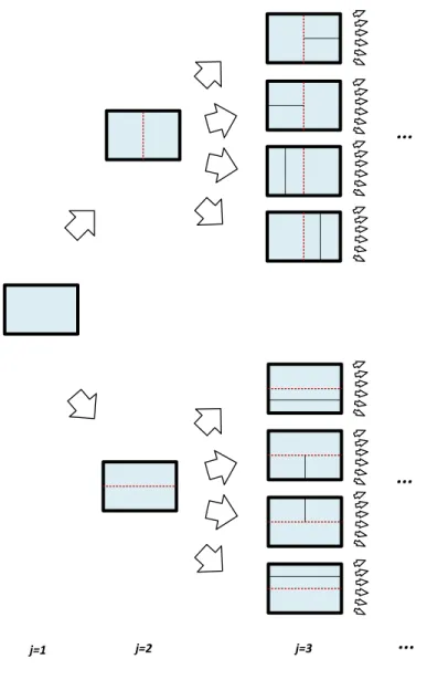
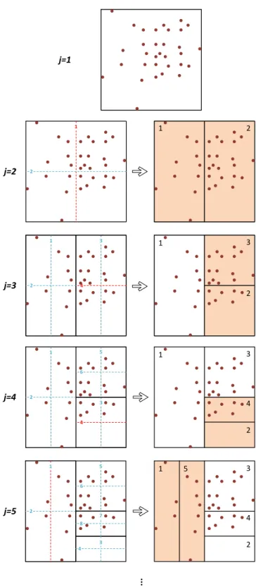
Figure 2.2 illustrates an example of binary sequential partitioning (BSP) in a 2-dimensional sample space. At j = 1, the algorithm starts with the entire sam-ple space. Based on the distribution of data, one of the dimensions is chosen for splitting the sample space using BP. At the beginning of each level j > 1, in

(41)

j=1 j=2 j=3

... ...

...

Figure 2.1: Example of mid-point binary partitioning scheme in 2D sample

space.

path gj = {cut2, cut3,· · · , cutj−1}, the sample space contains (j − 1) subregions

(p = 1,· · · , j−1), with subregion p having a volume of vp, and containing np data

points. There are (j−1)×Dpossibilities for thejth _{cut, from which one is randomly}

(42)

highest probabilities of being picked. For instance, in the example demonstrated in Figure 2.2, making the first cut in horizontal direction results in point distribution of

n(1) = 12 and n(2) = 20 for two halves. A vertical cut, on the other hand, produces

a slightly more unbalanced distribution with n(1) = 11 and n(2) = 21, and thus, it

has the highest probability of being randomly picked. Similar situation prevails in all consequent levels. In Figure 2.2, the dashed lines show all possibilities for the next cut, and the red dashed line shows the one that presents the highest probability.

To improve the quality of density estimation,M independent paths are tried at each level (M sample partitions). At each level j, path gjm = {cut2m, cutm3 ,· · · , cutmj−1},

(m= 1,· · · , M), the sample space contains (j−1) subregions (p= 1,· · · , j−1), with subregionphaving a volume ofvp, and containingnpdata points. There are (j−1)×D

possibilities for thejthcut. Enumerating the possibilities aspd= 11,· · · ,1D,· · · ,(j−

1)D, a conditional probability sjpd is calculated for each of these cuts as [9]:

sjpd(cutjpd|gj−1) = Cj−12 npΓ(n (1) pd)Γ(n (2) pd) Γ(np) (2.1)

where n(1)_pd and n(2)_pd are data points in each of the resulting halves due to the cut in subregion p along dimension d, and Cj−1 is a normalizing constant. The sum of all

(j−1)×Dconditional probabilities are normalized to unity to construct a probability mass function (PMF), which is used to make the random cut at level j in the chosen subregionpand dimensiond, to generate the new subregionp=j. Subsequent to the

(43)

1 1 2 5 6 7 8 4 3 1 2 5 3 6 4 j=3 j=4 j=5 3 j=2 1 2 j=1 ... 1 2 4 1 2 1 2 3 1 3 4 2 3 4 2 1 5

Figure 2.2: Calculating four new cut probabilities at each level, in 2D

(44)

cut, the data structures holding the information (the number of data points, volumes and coordinates) for the two new subregions, are updated accordingly. This process is repeated until either the best possible partition is obtained, or the number of cuts reaches the maximum value set by the user. Once the optimum partition is obtained, probability density is estimated for each subregion 1 ≤ p ≤ j (a D-dimensional bin), as np/(N vp). The best partition is the one that gives the lowest error between

the actual and estimated densities. However, since the actual density of the data is unknown for real datasets, the algorithm needs to be able to determine the best partition without relying on the knowledge of the actual density.

It has been shown in [9] that the log of the posterior distribution of a sample partition,

π(m) is a linear function of the Kullback-Leibler divergence (KLD) [36] [52] [53] [54] [55] between the actual and estimated densities, with a negative slope. Thus, in order to minimize the KLD, the algorithm uses the sample partition m with highest log(π(m)). To do so, for each sample partitionm ∈1,· · · , M, withj levels, a partition

score is defined as [9]:

score(m) = log(π(m)) =−βj+ log(B(n1+α,· · · , nj +α) B(α,· · · , α) )−

j X

p=1

nplog(|vp|) (2.2)

where α ∈ [0,0.5] and β ∈ [0.5,1] are two constants. vp and np are the volume and

the number of data points in the subregion p, respectively. B(u1,· · · , uK) denotes

the multivariate version of Beta-function [56] and is expressed in terms of Γ-function

(45)

maximum partition score at level j, we stop the BSP algorithm if the score does not improve within a further fixed number of partitioning levels, ∆j. A value of ∆j = 10 is used in this work. At this point, partition with maximum score, i.e. maximum

a-posterior (MAP), is chosen as the best partition.

2.2.1 BSP example

Consider the Gaussian mixture distribution in D dimensions,

X ∼

R X

r=1

crNr(µr,Σr) (2.3)

where Nr(µr,Σr) is a Normal distribution with the D-dimensional mean vector µr = (µ1, µ2, ..., µD)r; Σr = Cov[Xi, Xj]r is a D × D covariance matrix with i, j = 1,2,· · · , D, and cr are the mixture weights. Figure 2.3 presents the sample

data points for N = 20,000 for the case of R = 3 and D = 2, with the following parameters: µ1 = [2.25,5.40], µ2 = [2.60,5.65], µ3 = [2.8,5.15], Σ1 =     0.042 ₀ 0 0.042     , Σ2 =     0.072 ₀ 0 0.072     , Σ3 =     0.042 ₀ 0 0.042     c1 = 0.25, c2 = 0.4, c3 = 0.35.

(46)

x1 2.1 2.2 2.3 2.4 2.5 2.6 2.7 2.8 2.9 3 x2 4.8 5 5.2 5.4 5.6 5.8 6 Original 2D Data

Figure 2.3: Sample data (N = 20,000) from a trimodal bivariate normal

distribution. 3 2.8 2.6 2.4 x1 Actual Joint PDF 2.2 2 4.5 5 x2 5.5 20 30 40 0 10 6 Density

(47)

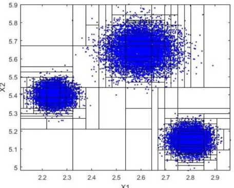
Figure 2.5: BSP cuts on the sample space of Figure 2.3, withN = 20,000 and M = 200. The number of BSP cuts is 182.

Figure 2.4 presents the actual density of the data in Figure 2.3, obtained from Eq. 2.3. Figure 2.5 presents the result of applying BSP on the sample space of Figure 2.3, with M = 200 sample partitions, and j = 182 cuts. This simple example clearly demonstrates how the BSP algorithm tends to make more cuts in the areas with more rapidly changing density, and few cuts in the areas with rather uniform distribution. Also, obviously, if a subregion is empty (local density is zero), it will never be further divided into smaller subregions.

(48)

2.3 Complexity

Reduction

Through

Copula

Transform

Further the true distribution is from uniform, the BSP algorithm requires more cuts to capture the structure of the data. This effect results in dramatic increase in the number of cuts and the deterioration of KLD values for high-dimensional data. The complexity arises due to the fact that in BSP the marginal distributions are learned together with the joint one. To reduce the number of time consuming cuts in the den-sity estimation in high-dimensional space, this section presents utilization of copula transform [41] [57] [58] as a method to map aD-dimensional density estimation prob-lem into the product of D one-dimensional marginal densities and a copula density. Each marginal density is estimated separately, and the results, along with density estimate of the copula, are used to estimate the joint density of the original dataset. The advantage of presenting the density in copula-transformed domain is that the transformed data will have uniform marginal distributions in the interval [0,1] [41], which leads to a significant reduction in the number of cuts in BSP in high dimensions and much better KLD.

In this work, I am using non-parametric copula, which is estimated directly from the distribution of marginal CDFs. For a random vector X = (X1,· · · , XD), BSP

(49)

f1(x1),· · · , fD(xD). The estimated PDFs are then used to build the marginal

cu-mulative distribution functions (CDFs), F1(x1),· · · , FD(xD)∈[0,1], where Fd(xd) = P(Xd≤xd). The resulting random variablesF1(X1),· · · , FD(XD) form the new

mul-tivariate dataset. As a result, the joint CDF of the sample dataset FX(x) can be

expressed as a standard copula C [41] as,

FX(x) = C(F1(x1),· · ·, FD(xD)) (2.4)

In copula domain, instead of using N samples of X = (X1,· · · , XD) to

per-form the BSP, we use N samples of the generated marginal CDFs as a copula-transformed dataset (F1(X1),· · · , FD(X1)) (a new N ×D dataset). The method

of BSP is then applied to this newD-dimensional dataset, to estimate the joint PDF

c(F1(x1),· · · , FD(xD)), wherec(u) = ∂ D

∂u1...∂uDC(u). The PDF for the original dataset, f(x), can then be calculated as [41],

f(x) = c(F1(x1),· · · , FD(xD)) D Y

d=1

fd(xd) (2.5)

Simulations show that in high dimensions, use of copula transform reduces the total number of cuts. More importantly, it reduces the number of computationally complex cuts required by the BSP algorithm in high dimensional space by as much as 98%, and substitutes them by computationally cheaper cuts in the marginal distributions.

(50)

Table 2.1

BSP with direct and copula-transformed cuts onD-dimensional space for various dimensions, forN = 20,000, M = 200.

Time unit is seconds. The number of cuts are shown as the sum of total marginal and copula cuts, as well as a pair in the parenthesis corresponding to each component.

D= 2 D= 32 D= 64

Direct Copula Direct Copula Direct Copula

Cuts 182 183 2938 1694 3648 3338

(96+87) (1614+80) (3266+72)

Time 13 19 2200 278 6018 552

KLD 0.045 0.018 33.5 0.19 72.5 0.31

Table 2.1 presents the number of cuts, the execution times and the KLD values of the direct and copula-transformed BSP for various dimensions, for a multivariate normal distribution. The synthetic dataset used in these simulations is a trimodal normal distribution for the first two dimensions, as shown in Figure 2.4. In 32 and 64-dimensional datasets, the third dimension is a unimodal normal distribution, and di-mensions four and higher have a bimodal normal distribution. This choice of datasets ensures adequate level of diversity in the marginal distributions. Significant from the data in Table 2.1 is the vast disparity between the KLD values for the direct and copula techniques for the high dimensional datasets.

(51)

x1 2.2 2.4 2.6 2.8 0 0.5 1 1.5 2 2.5 3 3.5 0 0.2 0.4 0.6 0.8 PDF CDF x2 5 5.2 5.4 5.6 5.8 0 0.5 1 1.5 2 2.5 3 3.5 0 0.2 0.4 0.6 0.8

Figure 2.6: Estimated marginal PDF and CDF, using copula transform,

forN = 20,000 and M = 200.

The number of BSP cuts for the two marginals X1 and X2 are 49 and 47,

respectively. -0.5 0 0.5 1 1.5 F1(x1) -0.5 0 0.5 1 1.5 F2(x2)

Figure 2.7: Distribution of the transformed random variablesF1(X1) and

(52)

F1(x1) 0.1 0.2 0.3 0.4 0.5 0.6 0.7 0.8 0.9 1 F2(x2) 0 0.1 0.2 0.3 0.4 0.5 0.6 0.7 0.8 0.9

1 Density estimation for c(F1(x1), F2(x2))

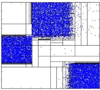
Figure 2.8: BSP cuts on copula-transformed sample space withN = 20,000

and M = 200. The number of BSP cuts is 87.

3 2.8 2.6 2.4 x1 Estimated Joint PDF 2.2 2 4.5 5 x2 5.5 20 30 40 0 10 6 Density

Figure 2.9: Estimated joint density, using copula transform with N =

(53)

T able 2. 2 BSP with copu la-transformed cuts on D -dimensional space, for three differen t opti ons. 1 : M = 200 for marginals, M = 200 for copula, Option 2 : M = 1 with MAP for marginals, M = 200 for copula, Option 3 : M = 1 with MAP for marginals, M = 1 for copula. D = 2 D = 32 D = 64 D = 128 D = 256 Option 1 Option 2 Option 3 Option 1 Option 2 Option 3 Option 1 Option 2 Option 3 Option 1 Option 2 Option 3 O pti on 1 Option 2 Option 3 Cuts 183 185 173 1694 1678 1625 3338 3262 3279 6666 6474 6485 13314 12914 12939 (96+87) (79+106) (79+94) (1614+80) (1543+135) (1517+108) (3266+72) (3152+110) (3147+132) (6569+97) (6249+225) (6302+183) (13237+77) (12649+265) (12693+246) Time 19 13 0.1 278 58 1 552 87 2. 6 842 197 10 1680 427 21 KLD 0.018 0.024 0.033 0.19 0.93 1. 33 0.31 1.62 2.02 1.51 4.22 3.90 1.59 6.84 6.59 (std) (0.0034) (0.0116) (0.0202) (0.0727) (0.4629) (0.5576) (0.0102) (0.4665) (0.7129) (0.4599) (0.7237) (0.7129) (0.3445) (1.0132) (0.7772) Cuts 293 294 284 2674 2654 2598 5277 5244 5153 10462 10400 10328 20837 20723 20621 (156+137) (152+142) (150+134) (2554+120) (2526+128) (2531+67) (5155+122) (5130+114) (5115+38) (10345+117) (10277+123) (10277+51) (20734+103) (20618+105) (20618+3) Time 111 44 0.5 1262 110 5 2475 169 10 4254 293 50 8857 485 99 KLD 0.007 0.008 0.01 0.068 0.077 0. 75 0.13 0.14 0.88 0.31 0.39 1.10 0.52 0.57 1.56 (std) (0.0014) (0.0018) (0.00508) (0.004) (0.0049) (0.4119) (0.0044) (0.0043) (0.4499) (0.1079) (0.1224) (0.4221) (0.0068) (0.0084) (0.4499)

(54)

Figure 2.6 to Figure 2.9 illustrate BSP through the application of copula transform for the same N = 20,000 data samples generated by Eq. 2.3. Figure 2.6 presents the estimated marginal PDFs and CDFs from BSP. Discontinuities in the PDF plots correspond to cuts from BSP process. Figure 2.7 presents two random variables

F1(X1) and F2(X2) in the transformed domain, which are in fact marginal CDFs

of X1 and X2. Figure 2.8 shows the copula-transformed sample space and the cuts

made by BSP process. For N = 20,000 and M = 200 the BSP has made a total of 183 cuts with 49 and 47 cuts for the two marginals X1 and X2, respectively. The

number of cuts for estimating the copula-transformed density in the 2-dimensional space is 87, a significant reduction from 182 cuts in the direct method. However, as expected, and seen in Table 2.1, for a low dimensional problem of d = 2 the overhead associated with the copula transformation far outweighs the reduction in the number of cuts in 2-dimensional space, which results in a higher execution time. Further, notice the difference between the cuts in Figure 2.5 with a higher number of cuts in the high density areas, and Figure 2.9, where most cuts are made away from high density areas. As we will see later, the cuts in the high density areas involve much higher computational complexity. The estimated joint density from the BSP algorithm is shown in Figure 2.9. The KLD between the true density in Figure 2.5 and the estimated density in Figure 2.9 is only 0.018.

(55)

2.3.1 Copula Transform and Sample Partition Diversity

One important effect of copula transformation is that for each of the marginals, cuts are made in one-dimensional space, meaning that at each levelj, there are onlyj−1 possible ways to make the next cut; alleviating the need for selecting a typically large value ofMto improve density estimation through increased path diversity. Simulation results for the 2-dimensional example in Figure 2.6 for marginals and Figure 2.8 for copula-transformed partitions are shown in Figure 2.10 (a) and (b), respectively. As seen from Figure 2.10 (a) after a relatively small number of cuts, the partition scores for allM = 200 sample partitions merge towards a single value, indicating that allM

independent paths eventually lead to the same or similar partitions. Plots in Figure 2.10 (a) also show that for two choices ofM = 1, (∆ for MAP and 2 for random cut from PMF), the scores are very close to, (and for most cuts even better than), the best score obtained withM = 200. Thus, for all marginals, BSP can be applied with only one sample partition,M = 1 with MAP for all j cuts.

For the case of BSP in copula-transformed multidimensional space, in Figure 2.10 (b) despite the fact that most of the sample partitions tend to converge at relatively small number of cuts j, the algorithm needs to process a large number of sample partitions to maintain a good diversity. The scores for two cases of M = 1 are very close to the

(56)

j 0 50 100 Partition Score 0 2000 4000 6000 8000 10000 12000 j 0 50 100 150 0 2000 4000 6000 8000 10000 12000 14000 16000 18000 20000 .BSHJOBM9 .BSHJOBM9 B C

M=1, MAP at each level j M=1, Random cut from PMF at each level j

C(F1(x1),F2(x2))

Figure 2.10: Partition scores with N = 20,000 and M = 200 sample

partitions for examples for (a) marginals in Figure 2.6, (b) copula in Figure 2.8.

with M = 200.

To further investigate the effect ofM on the density estimation, a set of simulations is performed with dimensions and distributions identical to Table 2.1, with two different dataset sizes. Simulation results are shown in Table 2.2, for a range of dimensions, from 2 to 256. In the basic setup (Option 1),M is 200 for all marginals as well as the

copula-transformed density estimation part. At each level j, the location of the next subregion cut is decided based on a random draw from the conditional probability in Eq. 2.1. A variation of the basic set up is Option 2, where M = 200 for the

copula-transformed part, but M = 1 for the marginals; i.e., for each of the marginals the algorithm only maintains one sample partition from beginning to the end of BSP.

(57)

At each levelj, subregion pwith the highest conditional probabilitysjp will be picked

for the next cut (MAP estimate). Finally, in Option 3, M = 1 for all marginals as

well as the copula-transformed estimation. In this setting, MAP estimate described above is used for the marginals only.

The values reported in this table are mean values obtained from multiple runs of the code: 32 runs forD= 2, 16 runs forD= 32, 8 runs for D= 64, and 4 runs for higher dimensions. The number of cuts are shown as the sum of marginal and copula cuts, with individual components presented as the pair in the parenthesis. The standard deviation corresponding to each KLD value is reported below it, in parenthesis. As can be seen in Table 2.2, for small dimension of D = 2 the variations in the estimation error (KLD) is small across the three options, even when the dataset is relatively small. Therefore, M can be set to 1 for both marginals and the copula to gain one to two orders of magnitude reduction in the computational complexity. For larger dimensions (32 and 64), with N = 20,000, the degradation in KLD is significant and use of options 2 and 3 become less attractive. However, for large dataset ofN = 100,000, with no appreciable increase in KLD, an order of magnitude reduction in computation time can be obtained by setting M = 1 for the marginals. A further one order magnitude reduction in computation time can be achieved, by setting M = 1 for both marginals and copula BSP, if an increase in KLD to more than 1.0 can be accepted.

(58)

be seen that even for high-dimensional cases, the BSP method (withOption 1 or 2)

is still able to provide good results, as long as the sample size is increased accordingly. In the following subsections, extended simulation results are presented, for a wider range of values of N, for the case of D = 64, to show how the estimation error is decreased by increasing the sample size.

Regarding computation time, it is observed that the time increases almost linearly with increasing dimensions. Computational complexity of the algorithm is discussed in further detail, in Sections 2.5 and 2.6.

2.4 Algorithm and Data Structures for BSP

2.4.1 Algorithm

When dealing with large, high-dimensional datasets, BSP method of density esti-mation can result in high computational complexity. The flowchart in Figure 2.11 illustrates my efficient implementation of the BSP through repeated evaluation of Eq. 2.1 and Eq. 2.2 in a loop. Similarly, the flowchart in Figure 2.12 illustrates the process of BSP using copula transformation, through evaluation of Eq. 2.4 and Eq. 2.5.

(59)

Start Read the input data

(N × D).

Create a sample space, bounded by Min and

Max of data in each dimension. Initialize all M sample partitions sptn1_,…,_sptnM

to the whole sample space. Variable initializations:

j=1; c=0; m=1; max_score=0; Next level: j = j + 1; Subregion p=1; Dimension d=1;

cutjm=(p,d);

Evaluate potential cut in subregion p along

dimension d.

For cutjm calculate the conditional probability

sjm(cutjm|gj‐1m). d = d + 1; d < D ? No p = p + 1; p < j‐1 ? No

Normalize (j‐1)×D values of sjm to create a

probability mass function (PMF).

Generate rcutjm by a random selection of

pair (p, d) from the PMF. Add a new subregion. Update sptnm_record.

Calculate score[m] for sptnm_.

Next sample partition: m = m + 1;

m <= M

No

max(score[]) > max_score ? No

c = c +1;

Calculate probability density in each

partition, for the sample partition with the

highest score (i.e., best_sptn).

c <= 10 ? Yes

max_score = max(score[]);

m_max = index(max(score[]));

best_sptn = sptnm_max_; c = 0; End Yes Yes Yes Yes Yes No j < jmax ? No 1 2 3 4 5 6 7 8 9 10 11 12 13 14 15 16

(60)

Start Read the

data (N × D) Initialize the dimension to

d=1;

Xd = Column d of data

Run BSP on Xd, to estimate

the marginal density fd(xd).

Next dimension: d = d + 1;

d <= D ?

Yes

data_cp = [F1(X1) … FD(XD)];

No

Using fd(xd), calculate the

marginal distribution Fd(xd).

Run BSP on data_cp, to estimate the joint density

of marginal distributions: c(F1(x1) , … , FD(xD))

Calculate the estimated joint density of data:

fX(x1, …, xD) = c(F1(x1), … ,FD(xD)) × f1(x1) × … × fD(xD) End 1 2 3 4 5 6 7 8

(61)

2.4.2 Subregion Evaluation Reduction

To improve the speed of the algorithm in the flowchart of Figure 2.11, an important observation is made. With reference to Eq. 2.1, at each level j, there is no need to calculate sjpd for all possible pd cuts. This is because the sjpd values corresponding

to all cuts, except the 2D potential cuts in the two recently modified subregions, are already calculated in the previous level, j −1. By properly storing and reusing these values, we can reduce the number of sjpd evaluations from (j −1)D to only

2D; which is a huge reduction in computation time, when level j becomes large, in high-dimensional problems. This simplification eliminates the loop over p in the flowchart of Figure 2.11. Figure 2.2 illustrates this computational simplification in 2D sample space. At each level j > 1 there are only two possible cuts (marked in blue and red dashed lines) for each subregion, with a total of 2(j −1) possible cuts. The red dashed line identifies the location earmarked for the actual cut at level j. The resulting two subregions separated by a solid black line, due to a cut at level j

are marked in beige. At each level j ≥3 , the algorithm only needs to calculate four new values of sjpd that belong to these two new subregions. All remaining possible sjpd values for cuts in subregions marked white are carried over from level j −1. In

Figure 2.2, the left column shows all the possible cuts, with red lines marking the actual cut. This leads to the new partition shown in the right column. For example,

(62)

probabilities associated with the possible cuts in subregions 1 and 3 (cut numbers 1, 2, 5, and 6) have already been calculated in the previous levelj = 4, and are available for reuse. So the algorithm only needs to evaluate the sjpd values for cut numbers 3,

4, 7, and 8.

2.4.3 Data Structures

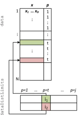
Main data structures for implementing the described BSP algorithm are listed in Table 2.3 [59]. The data structures are designed for efficient memory access and min-imum data movement. They are also designed for the ease of mapping into an efficient parallel processing paradigms of OPENMP® and MPI. All data structures are orga-nized for optimal column-major memory access, the method of choice in MATLAB®. Some of the data structures listed in Table 2.3 are for the purpose of estimation of one-dimensional marginal densities, while some others are exclusively designed for copula density estimation, and some structures are common for both estimations. At each level j, subsequent to a cut in one of the existing subregions, the data points in each of the two new subregions need to be identified and their total number counted and stored in the structure nSub. This is the most time consuming part of BSP algorithm for large and high-dimensional datasets. To reduce the computational complexity associated with this operation, theN×Dinput dataset structure,data, is augmented with an additional columnpto store the corresponding subregion number

(63)

for each of the data points. Then the whole structure is rearranged (partially sorted) such that all the points with the same subregion identity are stored in a contigu-ous block. The implemented scheme is shown in Figure 2.13. A pointer structure,

dataDistLimits, stores the indices for the first (marked green) and the last element (marked red) in each subregion. The efficiency of the proposed structure comes from the fact that when at level j, subregion t is cut, the algorithm only needs to sort the subset of the data structure marked as t. This partitioning scheme of dataset struc-ture,dataworks well for small dimensions less than 5. However, for larger dimensions, even the limited subregion sorting process requires movement of a large amount of multi-dimensional data. To reduce the data movement for dimensions larger than five, the structure shown in Figure 2.14 (a) is adopted where an intermediate data structuredataDiststores the indices todata. This way, the subregion sorting process involves a much simpler 2-column structure, instead of a D-column structure. In the optimized implementation of BSP using copula transform, for each of the marginals, a simpler structure, shown in Figure 2.14 (b), is used. Before processing each marginal

d, its corresponding column is copied fromdata todataMarginal. After processing,

dataMarginal will contain the CDF for that marginal, which is copied back to the corresponding column of data for copula processing, using the structure in Figure 2.14 (a).

(64)

T able 2. 3 List of main data structures used in copula-based im p le men tation of the BSP algorithm. Name Dimensions Description data N × D Con tains the whole input data se t o r copula-transformed data, i.e. N ro ws of D -dimensional data. dataMarginal N × 3 × M F or eac h of the M sample partitions, dataMarginal stores distribution of the marginal data for dimension d in partition subregions. The first column con-tains an index to the original data se t stored in data . T he second column con tains a cop y of column d of data . The third column stores the corresp ond-ing subregion n um b ers for the data from co lumn 2. After pro cessing of eac h marginal d , the second column of dataMarginal will con tain its marginal CDF, and is co pied bac k to the corresp onding column of data for copula pro ce ssin g. Continue d on next p age

(65)

T able 2.3 – Continue d fr om pr evious p age Dimensions Description N × 2 × M F or eac h of the M sample partitions, dataDist stores distribution of the data in the partition subregions. The first column con tains an index to the original dataset stored in data , and the second column stores the subregion n um b ers corresp onding to the indices from colum n 1. 2 × jmax × M Main tains p oin ters to the start and end en tries of eac h subregion in dataDist 2 D × jmax × M Stores co ordinates of the subregions. Eac h subregion is sp ecified b y its lo w er and higher b oundaries in eac h dimension. D × jmax × M Stores the calculated probab ilities for cutting eac h of the existing subre gions along an y of dimensions, at eac h lev el j . All v alues are in lo g domain. D × jmax Stores the lo g normalized probabilities from sjLog . M × 1 Stores the scores for sample partiti ons. Continue d on next p age

(66)

T able 2.3 – Continue d fr om pr evious p age Name Dimensions Description nSub jmax × M Stores the n um b er of data p oin ts in eac h of the subregions for eac h of M sample partitions. nSubMAP jmax × 1 Records the state of one column of nSub with the h ighest partition score, when the BSP meets the stopping crite ria. vSub jmax × M Stores the v olume of the subregions for eac h of the M sample partitions. vSubMAP jmax × 1 Records the state of one column of vSub with the h ighest partition score, when the BSP meets the stopping crite ria. bestDistMAP N × 2 Stores a subset of dataDist structure for the sample partition with the highest partition score. rCuts M × 1 Stores the subregion n um b er that is rando mly cut at eac h lev el j . Continue d on next p age

(67)

T able 2.3 – Continue d fr om pr evious p age Dimensions Description 2 × jmax × D Eac h columns of this stru cture corresp onds to one of the marginal densities and stores the final co ordinates of the subregions for the ma rginal sample partition with the highest partition score. jmax × D Eac h columns of this structure corresp onds to one of the marginal d ensities and stores the final estimated subr egion marginal densities. 2 D × jmax Stores the final co ordinates of the subregions, tak en from the partition with the highest partitio n score. jmax × 1 Stores the final v alues of the join t probabilit y densities, for the copula-transformed densit y estimation.

(68)

x ... N 1 1 1 p t t t 1 x1 … xD ... i1 i p=1 … ... ... x N 1 x1 … xD ... dataDist data ... p=j p=t i1 i2 p=1 … dataDistLimits p=j p=t … ... ... N dataMarginal p=1 … p=t … p=j data dataDistLimits _{dataDistLimits} i1 i iv iw iz 1 1 1 ... ... ... ... ... p xd ... ... ... ... ... ... i1 t i2 t 1 N iv iw iz ... ... ... p Index ... ... ... i1 t i2 t 1 ₁ 1 1 ... ... t … ...

Figure 2.13: Data structure extended, to store distribution of the data

points in subregions.

2.5 Density Estimation Simulation Results

This section presents the results obtained from MATLAB®simulation runs on a single Intel® Core i7-3820, 3.60 GHz, with 32 GB RAM, for the performance evaluations of the algorithm.

Density estimation is performed for the range of sample data sizes from N = 10,000 up to N = 1,000,000, and range of dimensions, from D = 2 up to D = 64. The simulations aim at examining the impact of different parameters on computational efficiency, measured in execution time, and estimation accuracy measured as KLD. Figure 2.15 presents the execution time and KLD for a 64-dimensional dataset versus

(69)

x ... N 1 1 1 p t t t 1 x1 … xD ... i1 i2 p=1 … ... ... x N 1 x1 … xD ... dataDist data ... p=j p=t i1 i2 p=1 … dataDistLimits p=j p=t … ... ... N dataMarginal p=1 … p=t … p=j (a) (b) data dataDistLimits dataDistLimits i1 i2 iv iw iz 1 1 1 ... ... _... _... ... xd p ... _... _... ... _... _... i1 t i2 t 1 N iv iw iz ... ... ... Index p ... ... ... i1 t i2 t 1 1 1 1 ... ... t … ...

Figure 2.14: Optimized data structure for storing distribution of data

points in subregions for (a) copula-transformed estimation where intermedi-ate data structure dataDiststores the indices to data, and (b) for each of the marginals, where the intermediate step is not required.

the sample sizesN, with the number of sample partitionsM as a parameter. Clearly, a larger sample dataset improves accuracy, at the cost of increased execution time. It can be seen that the execution time grows almost linearly with the sample sizeN.

(70)

The KLD between the actual density and the estimated density, on the other hand, decreases exponentially with sample size. For this particular example, increasing the sample size overN = 300,000 has little impact in improving the estimation accuracy. While the execution time increases linearly withM, the KLD exhibits small sensitivity to M. It is also seen that the choice of M = 1 for the marginals and M = 200 for the copula transformation results in no appreciable increase in KLD, with a six-fold reduction in computational complexity, when compared with the next closest case of M = 50 for both marginals and copula. A further 12-fold improvement in the execution time can be seen for the choice ofM = 1 for both marginals and the copula transformation. However, KLD on average remains higher than the case of M = 1 for the marginals and M = 200 for the copula transformation, by about a little more than 1.0. It also can be seen that for this case, due to the lack of diversity in the selection of the sample partitions, the KLD is relatively unstable across the range of

(71)

Ϭ Ϭ͘ϱ ϭ ϭ͘ϱ Ϯ Ϯ͘ϱ Ϭ ϱ ϭϬ ϭϱ ϮϬ Ϯϱ ϯϬ ϯϱ ϰϬ Ϭ ϭϬϬ ϮϬϬ ϯϬϬ ϰϬϬ ϱϬϬ ϲϬϬ ϳϬϬ ϴϬϬ ϵϬϬ ϭϬϬϬ <> dŝŵĞ; ƐĞĐͿ E

Time_M50_M50 Time_M100_M100 Time_M200_M200

Time_MAP_M200 Time_MAP_M1 KLD_M50_M50 KLD_M100_M100 _{KLD_M200_M200} KLD_MAP_M200 KLD_MAP_M1 (x 10 3 ) (x 103)

Figure 2.15: Execution time and KLD vs. sample size (N) for different

values ofM for a 64-D dataset.

2.6 Complexity Analysis and Parallelization

2.6.1 Complexity Analysis

The profiling of the algorithm presented in the flowcharts of Figure 2.11 and Figure 2.12 for Option 1, (M = 200 for marginals, M = 200 for copula), with N = 100,000

and D= 64 in Table 2.2 reveals that only 5% of the execution time is spent on the copula part. One reason is that only 2% of 5277 cuts are attributed to the copula. However, since a copula cut goes over all the 64 dimensions it is expected to have a much higher complexity (close to 64 times higher) compared to the complexity of a

(72)

marginal cut that goes over a single dimension; but the profiling results reveal that the average computational complexity for a copula cut is only about 2 times larger than that of the marginal cuts! There are two reasons for this ratio to be low. First, referring to the flowchart in Figure 2.11, it is noted that steps 10 to 14 in the flowchart are outside the loop for d, and therefore, executed only once for each iteration of m

irrespective of the value ofd. The profiling results further reveal that over 81% of the overall execution time is spent on the execution of these steps, with step 12 being the overwhelming contributor (over 78%). From the number of cuts in Table 2.2, it can be observed that on average every round of execution of steps 10 to 14 for a copula cut, there are 40 execution rounds of the same steps for a marginal cut. However, the overall complexity of one round of execution of these steps (in most part due to step 12) is more than three times less for a copula cut compared to a marginal cut. This is because in the copula case the fraction of cuts in the high density regions requiring time consuming count and sort operations across a large number of data points, and update of data structures in Fig 2.13 and 2.14 is far less than that for the marginals. This can be observed from Figure 2.8, where large blocks of high density areas in blue have no cuts. Further, for by the same token, the complexity of one round of execution of steps in the d loop, step 6 (involving the count of data points in each newly created subregion) to 9 is much less for a copula cut than for a marginal cut. From the preceding discussion, due to the fact that copula cuts form only a small fraction of the overall time, attempts to parallelize this part of the algorithm yields

(73)

no benefit. Therefore, the work presented later in Subsection 2.6.3 only focuses on parallelization over the marginals.

2.6.2 Effect of covariance matrix on performance of BSP

For illustration simplicity, in Section 2.2, for the Gaussian mixture distribution in Eq. 2.3, it was assumed that Σr[i, j] = 0 for i6=j. This is equivalent to Rr[i, j] = 0

for i = j and Rr[i, i] = 1, where Rr = (Σr)− 1

2Σ_r(Σ_r)− 1

2 is the correlation matrix.

In general, however, the correlation between marginals can have non-zero values. In order to investigate the effect of correlation matrix on performance of BSP, Table 2.4 presents the KLD and execution time performance of BSP for a range of correlation coefficients between 0 and 1, for the same 64-dimensional example studied before. From the data in the table, the KLD values remain small for correlation coefficients as high as 0.95. The contribution of copula to the total computation time increases linearly from about 6% to about 20% for the change in the correlation coefficient from 0 to 0.95. The increase in the number of cuts follows the same trend.

It should be noted that in the multivariate analysis, where there is high correlation between the marginals the method of principal component analysis (PCA) [60] can be used to transform the dataset into a new set of variables in smaller number of dimensions (principal components) that are uncorrelated. The method of BSP can

(74)

Table 2.4

Impact of correlation on computation time and estimation accuracy (N = 100,000,D= 64).

Time Cuts KLD

R Marginal Copula Total Marginal Copula Total

0 2315 160 2475 5155 122 5277 0.13 (93.7%) (6.3%) 0.2 2288 178 2466 5106 178 5284 0.13 (92.8%) (7.2%) 0.4 2282 239 2521 5078 246 5324 0.14 (90.5%) (9.5%) 0.6 2282 256 2538 5133 269 5402 0.23 (89.9%) (10.1%) 0.8 2280 402 2682 5133 464 5597 0.15 (85.0%) (15.0%) 0.9 2352 494 2846 5133 579 5712 0.16 (82.6%) (17.4%) 0.95 2302 574 2876 5133 671 5804 0.18 (80.0%) (20.0%) 1.0 2322 6930 9252 5148 4177 9325 14.71 (25.1%) (74.9%)

2.6.3 Parallelization

The proposed algorithm in the flowcharts of Figure 2.11, and the data structures in Table 2.3, Figure 2.13 and Figure 2.14, have been designed suitably for the ease of parallelization around BSP parameters; dataset elements 1 ≤ n ≤ N, sample partitions 1 ≤ m ≤ M, dimensions 1 ≤ d ≤ D and subregions 1 ≤ p ≤ j −1. In this section, the discussion is limited to the coarse-grain parallelization around

m and d. Fine-grain parallelization over data sample n is best achieved through massively parallel architectures of graphical processing unit (GPU) and is limited to

Offline and Online Density Estimation for Large High-Dimensional Data

Digital Commons @ Michigan Tech

Digital Commons @ Michigan Tech

Offline and Online Density Estimation for Large High-Dimensional

Offline and Online Density Estimation for Large High-Dimensional

Data

Data

Dedication

To my dear mother Raziyeh and my loving father Iraj,

Contents

List of Figures

List of Tables

Preface

Acknowledgments

List of Abbreviations

Abstract

Chapter 1

Introduction

1.1

Motivation

1.2

Background

1.3

Outline

Chapter 2

Density Estimation in

High-dimensional Domain

2.1

Binary partitioning

2.2

BSP Algorithm

2.2.1

BSP example

2.3

Complexity

Reduction

Through

Copula

Transform

2.3.1

Copula Transform and Sample Partition Diversity

2.4

Algorithm and Data Structures for BSP

2.4.1

Algorithm

2.4.2

Subregion Evaluation Reduction

2.4.3

Data Structures

2.5

Density Estimation Simulation Results

2.6

Complexity Analysis and Parallelization

2.6.1

Complexity Analysis

2.6.2

Effect of covariance matrix on performance of BSP

2.6.3

Parallelization