United States Military Academy
United States Military Academy
USMA Digital Commons
USMA Digital Commons
West Point Research Papers
Fall 11-25-2019
A Collaborative Visual Localization Scheme for a Low-Cost
A Collaborative Visual Localization Scheme for a Low-Cost
Heterogeneous Robotic Team with Non-Overlapping Perspectives
Heterogeneous Robotic Team with Non-Overlapping Perspectives
Benjamin Abruzzo
CCDC Armaments Center, U.S. Army ARDEC , Picatinny Arsenal, NJ, [email protected]
David Cappelleri
Purdue University, West Lafayette, IN
Philippos Mordohai
Stevens Institute of Technology , Hoboken, NJ
Follow this and additional works at: https://digitalcommons.usmalibrary.org/usma_research_papers Part of the Artificial Intelligence and Robotics Commons, and the Robotics Commons
Recommended Citation
Recommended Citation
Abruzzo, Benjamin; Cappelleri, David; and Mordohai, Philippos, "A Collaborative Visual Localization Scheme for a Low-Cost Heterogeneous Robotic Team with Non-Overlapping Perspectives" (2019). West Point Research Papers. 280.
https://digitalcommons.usmalibrary.org/usma_research_papers/280
This Conference Proceeding is brought to you for free and open access by USMA Digital Commons. It has been accepted for inclusion in West Point Research Papers by an authorized administrator of USMA Digital Commons.
Proceedings of the ASME 2019 International Design Engineering Technical Conferences and Computers and Information in Engineering Conference IDETC/CIE2019 August 18-21, 2019, Anaheim, CA, USA
IDETC2019-97377
A COLLABORATIVE VISUAL LOCALIZATION SCHEME FOR A LOW-COST
HETEROGENEOUS ROBOTIC TEAM WITH NON-OVERLAPPING PERSPECTIVES
Benjamin Abruzzo Stevens Institute of Technology
Hoboken, NJ 07030 U.S. Army ARDEC Picatinny Arsenal, NJ 07806 benjamin.a.abruzzo.civ at mail.mil
David Cappelleri Associate Professor School of Mechanical Engineering
Purdue University West Lafayette, IN 47907-2088
dcappell at purdue.edu
Philippos Mordohai Associate Professor Department of Computer Science
Stevens Institute of Technology mordohai at cs.stevens.edu
ABSTRACT
This paper presents and evaluates a relative localization scheme for a heterogeneous team of low-cost mobile robots. An error-state, complementary Kalman Filter was developed to fuse analytically-derived uncertainty of stereoscopic pose measure-ments of an aerial robot, made by a ground robot, with the iner-tial/visual proprioceptive measurements of both robots. Results show that the sources of error, image quantization, asynchronous sensors, and a non-stationary bias, were sufficiently modeled to estimate the pose of the aerial robot. In both simulation and ex-periments, we demonstrate the proposed methodology with a het-erogeneous robot team, consisting of a UAV and a UGV tasked with collaboratively localizing themselves while avoiding obsta-cles in an unknown environment. The team is able to identify a goal location and obstacles in the environment and plan a path for the UGV to the goal location. The results demonstrate local-ization accuracies of 2cm to 4cm, on average, while the robots operate at a distance from each-other between 1m and 4m.
Supplemental Material1
This paper is accompanied by a video of the robot po-sition and the IMU perceived popo-sition: https://youtu. be/RNa_ndlBlSU. The source code used for these
exper-1Unclassified. Distribution A. This publication is approved for public release
distribution is unlimited.
iments can be downloaded here: https://github.com/
benjaminabruzzo/idetc2019_code.
1 Introduction
In the growing body of research on collaborative robotics a variety of application spaces are investigated, including aerial exploration and navigation, SLAM, manipulation, infrastructure inspection and maintenance, heterogeneous teams, and disaster response. A major challenge facing teams is the task of local-izing relative to other team members in a reliable manner which allows them to share knowledge or measurements about the envi-ronment. Common solutions to this challenge fall into one of two types: 1) registering fixed landmarks, jointly observable by team-mates when measured from different perspectives [1–8], or 2) directly observing teammates to calculate relative poses [9–15]. For example, Schmuck and Chli [7] focus on mapping an out-door area using a single UAV over four distinct flight paths. The four flight paths were used to simulate four distinct ‘vehicles’ by replaying the captured data synchronously on a ground station to aggregate the observations of the UAVs, merge maps, and man-age loop closures. By supplying the optimized information back to the UAVs, the simulated UAVs can use the provided informa-tion to better localize from the collective key frames. In [6] two UAVs, each equipped with a single camera, aim to maximize the overlap of their forward facing cameras to enable the estimation
1 INTRODUCTION
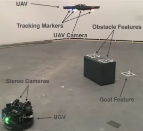
FIGURE 1: Heterogeneous team in unknown environment with an obstacle. of the essential matrix. From the essential matrix, relative po-sition and orientation can be extracted and used to maintain a formation between the two vehicles.
In the previous two cases, the jointly observable features in the environment are used as the reference to relatively localize the UAVs. Alternatively, Dias et al. [11] and Teixeira et al. [15] approached pose estimation by directly observing nearby UAVs using on-board monocular cameras. In [11], illuminated spheres were affixed to three UAVs to aid in detection and pose estima-tion. Vehicle identification was accomplished through a unique flashing frequency of one of the affixed markers on each UAV. In flight, one UAV was able to maintain a relative pose to the other two stationary UAVs. In contrast, Teixeira et al. [15] use colored LEDs with spherical diffusers in a known constellation to aid in detection of a dependent UAV by a supervisor UAV. Both meth-ods use the perspective 3-point (P3P) algorithm to calculate the pose estimates from the observed markers. In all four of these ex-amples, each team was composed of homogeneous UAVs which are limited by power, computation, and lifting capacity.
Several authors have attempted to address the limitations of UAV teams by implementing a heterogeneous air-ground team. Such a configuration provides complementary capabilities; the additional UGVs can operate for much longer periods, carry sig-nificantly more cargo, or even have an attached manipulator. For example, the authors in [16] sought to minimize the total explo-ration time of a UAV-UGV team with a strong focus on the tra-jectory planning aspect of collaboration. By combining terrain classes with a 2.5D elevation map generated by the UAV to plan a feasible path for the UGV, which was then executed by a hu-man pilot. Their work led to progress in collaborative robotics, but the fact that the UGV is manually operated highlights that the problem is not completely solved. Our work aims to make an additional step towards collaborative, full automation. In sim-ilar works, a UAV was used to explore and unknown environ-ment to generate a feature based map which was then aligned
to a similar map created by a ground vehicle configured with a point-cloud generating sensor (RGBD [2], LiDAR [3], laser scanner [4], monocular camera [5], or a camera and scanner [1]). After the resulting maps were aligned, the robots could calcu-late relative pose between vehicles. In all six of these publica-tions, the robots continued to operate independently even after the maps were explored or aligned. The benefit of using the en-vironment to indirectly localize is the freedom of motion away from any field of view constraints. However, this freedom comes at the cost of localization ambiguity and introduces a require-ment for the team to carry compatible sensors with the ability to measure the same features. Measurements from these sensors are then used to align maps generated from the different perspec-tives, but will fail entirely if the observed regions never overlap.
A solution which avoids map alignment involves one robot observing another to then calculate the relative pose directly. For example, in both [13] and [14] a UAV conducted an explo-ration trajectory to create a map of the environment, and then re-turned to hover above the UGV. The UGV in the system carried a vertically-oriented, 2D fiducial marker to enable simple detec-tion and tracking by the UAV while the UGV was in modetec-tion. While in motion, the UAV continued to estimate its own pose and thus could provide pose estimates to the UGV to assist while moving through the environment. Other authors in [11], [12] and [15] avoid the need for the large, oriented 2D markers which are only observable from a specific perspective used in [10], [13], and [14] by equipping robots with active, light-emitting markers, which are then used P3P for fast visual pose estimation.
For relative pose determination we have developed a method most similar to [17], in which a UAV carries spherical diffusers covering uniquely-colored LEDs to aid in visual detection. These markers are observed by a stereoscopic camera system that esti-mates the 6DOF pose of the UAV. This is different than in [12], which used non-diffused LEDs as the identifying markers. LEDs are both small and directional, which imposes constraints on viewing direction and filtering images to reduce noise. Using colored spheres instead of LEDs enables a wider range of view-ing perspectives as well as a larger physical feature to detect. While the authors in [17] fix the location of cameras to be used as an alternative to a motion capture system, we have mounted the cameras onto the UGV to enable a mobile solution to local-ization.
In our team, the UGV is completely reliant on the UAV for the map of obstacles and goal locations, whereas the UAV is reliant on the UGV for position relative to a global reference frame. This interdependence differs from the map-alignment style works presented earlier. Robots in our team do not mu-tually observe the same features or landmarks, therefore, such techniques would not be applicable. As the UGV moves, it con-tinues to provide position information to the UAV, while the UAV ensures there are no obstacles in the path of the UGV. Finally, we have developed a complementary Kalman filter to
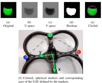
simultane-2 SYSTEM OVERVIEW AND APPROACH (a) Original (b) U space (c) V space (d) Boolean (e) Circled
(f) Colored, spherical markers and corresponding axes of the UAV defined by the markers.
FIGURE 2: Circle detection of spherical markers for triangulation. ously update the pose estimates of the UGV and UAV by com-bining the high-frequency proprioceptive sensors on each robot with the low-frequency relative pose measurements of the stereo-scopic cameras.
The main contribution of this work is the presentation and evaluation of a novel relative localization scheme using low-cost, heterogeneous, mobile robots which are able to share environ-mental observations and pose estimates while navigating in an unknown environment without requiring correspondences of mu-tually visible features or landmarks. While we focus on visual perception, the results of this work are not limited to computer vision; application of these methods could easily be extended to other combination of robots or sensors.
2 System Overview and Approach
As mentioned previously, we propose a collaborative lo-calization scheme for low-accuracy, low-cost robots. Figure 1 shows an example configuration of such a team. Specifically, there is a UGV which carries a calibrated and software-rectified stereoscopic camera system with an upward tilt. This allows the UGV to directly observe the second member of the team, a UAV. To simplify recognition and tracking of the UAV, uniquely-colored, illuminated, spherical markers are attached to it. The UAV is equipped with an IMU to maintain stability while in flight and a calibrated, downward-facing camera to observe the environment. However, it lacks a sensor to provide localization relative to an external reference frame. In this configuration, nei-ther vehicle is able to directly observe the same aspects of the environment.
2.1 Stereoscopic Measurements
To localize the UAV, the cameras on the UGV convert the RGB color images into YUV color coordinates, which are then
thresholded to screen for the different colored markers. Morpho-logical processing, specifically, erosion and dilation, are applied to reduce background noise and generate clean boolean images corresponding to each marker color. Minimum radius circles are circumscribed around the resulting blobs to determine marker centroids. Figure 2 shows the resulting boolean image of a de-tected marker and the circle fit around the marker.
Marker occlusion is rare due to the viewing angle of the UGV, but even in the presence of partial occlusion the circle finding process still matches a circle by circumscribing the color matched pixels, see Figure 2. Since the center of a 3D sphere projects to the center of a 2D circle in images, fitting circles to detected blobs allows us to assume the center of the circle lies on a ray through the actual center of the marker. Beyond simple im-age discretization, circle finding enables sub-pixel determination of the marker center.
Using triangulation, the 3D position of an ideal point marker in the camera frame,cammppp, can be calculated as shown in Equa-tion (1). We assume that the UGV-mounted stereoscopic cameras are calibrated and rectified, which leaves image quantization as the predominant source of error when determining the 3D posi-tion of a point by stereoscopic triangulaposi-tion [18]. Because the images are fully rectified (in software),yL=yR=y, thus the Ja-cobian of the triangulation equations is Equation (2). In both Equations (1) and (2), xL,xR, yL, andyR are the left and right pixel coordinates of the point marker’s projection onto the image plane, d =xR−xL is the disparity between two corresponding pixel coordinates in the left and right images,bis the baseline be-tween cameras, and fis the focal length of the cameras. Once the 3D positions of the markers are known, computing the body axes and heading angle of the UAV is trivial using vector operations. These values are calculated in the frame of the stereoscopic cam-eras, which are then be transformed into the UGV frame prior to inclusion in further pose estimates.
cam mppp= X Y Z = b 2d(xL+xR) b 2d(yL+yR) f b d = b 2d(xL+xR) by d f b d , (1) cam mJ= ∂fX ∂xL ∂fX ∂xR ∂fX ∂y ∂fY ∂xL ∂fY ∂xR ∂fY ∂y ∂fZ ∂xL ∂fZ ∂xR ∂fZ ∂y = −bxR 2d2 bxL 2d2 0 −by d2 by d2 b d −b f d2 b f d2 0 (2)
2.2 Complementary Kalman Filters for UAV and UGV 2 SYSTEM OVERVIEW AND APPROACH
2.2 Complementary Kalman Filters for UAV and UGV To simplify the propagation of uncertainty from image to vehicle coordinate systems, we approximate the non-Gaussian errors in measured image coordinates as Gaussian, as in [19]. Image uncertainties are propagated linearly to the 3D triangula-tion calculatriangula-tions. In general, the output covariance matrix,Σo, of a function,g, is given by:
Σo=JgΣiJgT, (3)
whereΣiis the covariance of the input andJgis the Jacobian of g. We use this first-order method of uncertainty propagation to derive error covariance matrices from the triangulation error of image features to 3D position covariances of the active markers. These marker positions and covariances are then used to derive the position and heading angle of the UAV and the covariances of those values.
Complementary filtering is a method for combining redun-dant measurements and is most useful in situations where the spectral properties of the measurements are different [20], [21]. This is beneficial to the configuration of our team where both ve-hicles have an inertial/odometric sensor package which indepen-dently operate at much higher frequencies than the stereoscopic cameras and also at different rates from each other. The Comple-mentary Kalman Filter (CKF) that we have developed is an indi-rect filter that estimates the errors in the vehicle states. This fil-ter operates on the error-state vector between the estimated pose computed by the high-rate, body-centered inertial sensors and the low-rate relative measurements of the stereoscopic cameras. In general, this type of configuration limits the need to develop highly detailed dynamical models and decreases the frequency that the filter needs to update [22].
For our system, we assume that the firmware maintains the flight stability of the UAV and that our filter will only be used for higher level navigation and communication of detected ob-stacles to the map for the UGV. The stability controller of the UAV manages the roll and pitch angles freeing our filter from estimating those two states. Thus, the filter is only concerned with the three Cartesian coordinates (x, y, z), and the heading angle (ψ). The UAV firmware also provides a lateral velocity measurement through a combination of the on-board IMU mea-surements in conjunction with optical-flow odometry from the downward-facing camera as well as an altimeter for altitude mea-surements. As part of the IMU, the gyroscopic compass gener-ates the directly-measured heading value, but has a slow walking-bias term (β) which is included in the augmented state vector, uavppp=
uavxuavyuavzuavψ β T
. Lastly, the operational dynam-ics of the UAV maintain slow angular rates with regard to head-ing, so higher order terms are neglected.
The stereoscopic cameras provide a direct measurement of
the pose of the UAV in the UGV frame, ugvuavppps, which is trans-formed into the global frame, gppp
s, using the most recent esti-mates of the UGV position, uavgppps, and corresponding rotation matrix,uavgRRR. In the time between the camera measurements, the estimated states of the vehicles, uavgpppˆ andugvgppp, are updated di-ˆ rectly with the time integration of the high-frequency sensors. Without the external reference, the errors of the high-frequency inertial/odometric sensors accumulate and the resulting pose es-timates diverge from the actual states of the vehicles.
When a new camera based relative measurement is calcu-lated, first the estimated relative pose between the vehicles,∆p,ˆ is computed from the most recently estimated position of both vehicles:
∆ppˆp= uavgppˆp− g ugvpppˆ
. (4)
The measurement error vector, δpp˜p, is the difference between these two measurements:
δppp˜=gppps−∆pˆpp (5)
Because the slowest sensor contributing to the filter is the stereo-scopic measurements, the filter is only updated when each new stereoscopic measurement is made. At each update the optimal error state estimate,δppˆpk+1, is computed by Equation 6,
δppˆpk+1=FFF·δppˆpk+KKKk·δppp˜. (6)
Where FFF is the matrix of the error state dynamics, andKKKk is the Kalman gain calculated in the standard fashion [21]. The optimal error state estimate is used to proportionally update the estimated states for both vehicles. This estimate is updated at the time of each new image in real time at the frame-rate of the stereoscopic cameras (in our experiments, this occurs at approx-imately 10 Hz).
Similar to the UAV states, the UGV states estimated by the filter are the two 2D planar Cartesian coordinates and the head-ing angle,ugvppp= g
ugvxugvgyugvgψT. Vehicle-level wheel odome-try is used to generate the high-rate kinematic trajectory between stereoscopic updates. The simplicity of the vehicle models is one of the benefits from the complementary filtering approach [22]. Additionally, between updates of the CKF, the measurements from the high-frequency sensors are used to compute the most up-to-date estimates of vehicle poses in the relative and global frames. These estimates can be sequentially applied to transform measurements made in the UAV camera frame to the UGV or global frames as necessary.
2.3 UAV Control 3 ACCURACY OF RELATIVE MEASUREMENTS 0 10 20 30 40 50 60 70 80 90 1 1.5 2 2.5 3 3.5 4 4.5 Simulation X [m] 00.5 1 1.5 2 2.5 3 3.5 Experiment X [m]
Goal Location Ground Truth CKF Est Sim CKF Est Exp
0 10 20 30 40 50 60 70 80 90 time [s] -0.5 0 0.5 1 1.5 Simulation Y [m] -1.5 -1 -0.5 0 0.5 Experiment Y [m] 0 10 20 30 40 50 60 70 80 90 0.5 1 1.5 2 Simulation Z [m] 0 0.5 1 1.5 Experiment Z [m] 0 10 20 30 40 50 60 70 80 90 time [s] -60 -30 0 30 60 90 120 Simulation Yaw [m] -120 -90 -60 -30 0 30 60 Experiment Yaw [m] Experiment Simulation
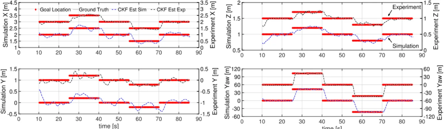
FIGURE 3: Simulation and experiment trajectories of UAV controlled by static UGV. Red diamonds are the goal poses for the UAV and the gray solid lines are the ground truth measurements from the Vicon motion capture system. The blue dashed lines are the estimated trajectory of the UAV in simulation and the black dashed lines are the estimated trajectories from an experiment. Note: the simulation data are offset from the experiment data for clarity.
2.3 UAV Control
The logic used for autonomous control is designed to drive the velocity of the UAV to zero and the estimated global pose of the UAV, uavgppp, to the desired global pose,ˆ uavgpppd = g
uavxduavgyd uavgzd uavgψd T
. The controller is shown in Equation (7), whereuavUUUis the control vector in the body frame,Kpand Kvare experimentally determined, constant gains applied to the pose and velocity errors, anduavgRRR(ψˆ)is the rotation matrix re-quired to convert from the global frame to the UAV body using the most recent estimate ofuavψ. A purely proportional control law would allow the UAV to overshoot the desired position due to the lateral dynamics of the UAV, which tends to allow ‘slip-ping’ when the UAV is completely horizontal. This is due to the inertia of the UAV, which would only be counter-acted by tilting the UAV to stop the lateral velocity. For this reason the UAV con-trol logic includes terms that drive the lateral velocities to zero but does not include angular or altitude velocities. While this is a simplistic controller, UAV modeling and control is not the main focus of this work, and a wide variety of control schemes could be implemented instead, e.g. [23, 24].
uavUUU=K
p·uavgRRR(ψˆ)·(uavgpppd−uavgpˆpp)−Kv· uav ˙ x ˙ y (7)
3 Accuracy of Relative Measurements
In physical experiments, vehicle position and orientation ground truth are measured by a Vicon motion capture sys-tem. A Parrot AR.Drone 2.0, which costs $300, is used as the aerial robot. Stability of the UAV is firmware-controlled by the manufacturer-developed Extended Kalman Filter autopilot using the on-board IMU [25]. Sensor measurements are communicated via a WiFi connection between the UAV and the UGV using the
SDK provided by the Parrot organization and the ROS wrapper developed by Simon Fraser University [26]. We assume any la-tency from networking and communication is small and will not contribute significantly to the errors of the system.
The ground vehicle is a modified version of the low-cost “Tortoisebot” developed at Stevens Institute of Technology [27] and costs under $2500. On the UGV, the Robot Operating Sys-tem (ROS) is used as the coordination framework for fusing sen-sors and estimated poses. The pair of cameras carried by the UGV are PointGrey Chameleon cameras (1288x964) with Fuji-non 70oFOV lenses. The cameras are separated by a baseline of 15 centimeters and they are calibrated using the ROS cam-era calibration package. Both the AR.Drone and the Turtlebot were modeled in Gazebo to simulate this configuration using the same ROS/C++ software developed on the actual robots.
TABLE 1: Magnitude of position and yaw errors of the UAV estimates from the simulation and experiment shown in Figure 3
UAV error x [m] y [m] z [m] ψ[deg] Simulated: mean 0.018 0.015 0.014 0.5 max 0.042 0.039 0.039 3.6 Experimental: mean 0.019 0.008 0.010 0.6 max 0.078 0.028 0.045 4.0
To demonstrate the closed loop performance of the team, we conducted experiments with the UAV in flight while a station-ary UGV provides position and orientation localization. After lifting off, the UAV was guided through a series of way-points, exercising changes in position and yaw angle. This experiment was designed to assess whether the CKF will accurately estimate Unclassified. Distribution A. This is approved for public release distribution is unlimited.
4 COOPERATIVE MANEUVERS
the states of the UAV. This type of experiment will also show if the control law for the UAV will suitably guide the UAV to poses prescribed by the UGV. Lastly, we want to determine if the simulation of the UAV accurately depicts reality based on the assumptions made in developing the team and our approach.
For each iteration of this experiment, the UAV lifted off from a location in front of the UGV and was guided by the UGV through a set of way-points while the UGV remained station-ary. Throughout the experiment, both vehicles were observed by the Vicon motion capture system, though these data were only used to provide the ground-truth of the landmarks’ and robots’ positions. An example of the measured and estimated states of the UAV is shown in Figure 3. These plots show that the UAV controller will converge on the goal location within a few sec-onds. The average and maximum errors of the estimated UAV pose for both experiments are compiled in Table 1. In both sim-ulation and experiment, the errors are largest in thexdirection due to triangulation from stereoscopic measurements, which are least accurate along the optical axis of the cameras. The errors in Table 1 reflect a strong agreement between simulation and real experiments.
4 Cooperative Maneuvers
Based on the results of the relative measurement experi-ments described in Section 3, a new set of experiexperi-ments were de-signed with both robots moving in order to showcase cooperative maneuvers for the robot team. The environment for these exper-iments included a physical obstacle between the UGV starting and goal locations. To simplify detection of obstacles and goal locations, two fiducial landmarks [28, 29] were placed on top of the barricade while the third was placed on the opposite side of the barricade from the UGV to provide a goal location. Addition-ally, these landmarks were chosen to be specifically unobservable by the UGV, forcing the UGV to rely upon the UAV to provide in-formation about the environment. This configuration highlights the complementary nature of a heterogeneous UAV-UGV team, especially with regard to the perspective of each robot relative to the environment.
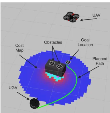
For planning, we used the standardROS move basepackage. Using a well known and accepted method allowed us to focus on the relative localization and cooperative nature of the team. The global planner used by the UGV was the defaultnavfn plan-ner based on the Dijkstra algorithm for computing the naviga-tion funcnaviga-tion. The cost map for the planning algorithm was con-structed using the locations of the fiducial landmarks as observed by the UAV. Finally, obstacle avoidance was implemented using the Dynamic Window Approach local planner of themove base package. Figure 4 is a snapshot of an experiment at the moment when the UAV has already created the map and the UGV has charted a path but has not yet started moving. Figure 5 shows the estimated path of the UGV overlaid with the actual path of the
UAV Obstacles Planned Path UGV Cost Map Goal Location
FIGURE 4: Still frame from experiment at the moment that a plan for the UGV has been computed but before the UGV begins to move. The inset shows the planned trajectory of the UGV around the obstacles.
UGV during trial 5.
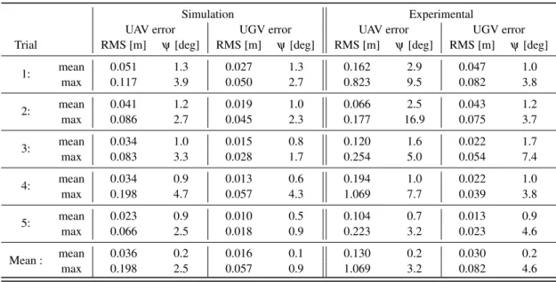
Table 2 presents a compilation of five trials of this experi-ment, both in simulation and in the laboratory. The errors re-ported in Table 2 are the differences calculated between the esti-mated position and orientation of each vehicle and the pose data from the Vicon motion capture system. Each row corresponds to a distinct trial and for each trial the average and maximum errors of the estimated position of each vehicle is reported. The maxi-mum and average across all trials is included in the final row of the table. The trials were conducted on two different days, and each trajectory and obstacle configuration is shown in Figure 6. For each trial, the simulation is configured to match the initial configuration of the corresponding physical experiment with re-gard to initial poses of vehicles and obstacles.
In Figure 6, the trajectory in trial 4 appears to have an anomalous path compared to the other trials; this is due to the ini-tial conditions and the path optimization. In this trial, the UGV moved closer to the obstacles, and as a result the recalculated minimum cost path diverged from the other trials. Additionally, in both Trials 1 and 4 the maximum error of the UAV position is significantly higher than that of the other trials. In these two cases, during the experiment, the UAV was briefly outside the field of view of the UGV, causing the estimate to drift, after the
4 COOPERATIVE MANEUVERS
TABLE 2: Position and yaw errors of the simulated and actual UAV and UGV pose estimates from collaborative experiments. Simulation Experimental
UAV error UGV error UAV error UGV error Trial RMS [m] ψ[deg] RMS [m] ψ[deg] RMS [m] ψ[deg] RMS [m] ψ[deg]
1: mean 0.051 1.3 0.027 1.3 0.162 2.9 0.047 1.0 max 0.117 3.9 0.050 2.7 0.823 9.5 0.082 3.8 2: mean 0.041 1.2 0.019 1.0 0.066 2.5 0.043 1.2 max 0.086 2.7 0.045 2.3 0.177 16.9 0.075 3.7 3: mean 0.034 1.0 0.015 0.8 0.120 1.6 0.022 1.7 max 0.083 3.3 0.028 1.7 0.254 5.0 0.054 7.4 4: mean 0.034 0.9 0.013 0.6 0.194 1.0 0.022 1.0 max 0.198 4.7 0.057 4.3 1.069 7.7 0.039 3.8 5: mean 0.023 0.9 0.010 0.5 0.104 0.7 0.013 0.9 max 0.066 2.5 0.018 0.9 0.223 3.2 0.023 4.6 Mean : mean 0.036 0.2 0.016 0.1 0.130 0.2 0.030 0.2 max 0.198 2.5 0.057 0.9 1.069 3.2 0.082 4.6 -0.5 0 0.5 1 1.5 2 2.5 3 3.5 4 UGV x position [m] -0.5 0 0.5 1 1.5 UGV y position [m]
goal obstacle actual path estimated path
-0.5 0 0.5 1 1.5 2 2.5 3 3.5 4
Distance along trajectory [m]
-0.02 0 0.02
Position error [m] ugv estimate error
FIGURE 5: (Top) UGV estimated and actual trajectory for trial 5. Coordinates are relative to the UGV’s starting orientation. The dashed circles represent the circumscribed physical footprint of the UGV and the goal landmark.(Bottom) Error of UGV estimate as a function of distance traveled.
UAV returned to the FOV of the UGV, the errors recovered. This can be seen by the comparability of the average errors across all trials for the UAV position. At the conclusion of each trial, the error of the UGV position is approximately 2% or less of the distance traveled.
While our experiment includes specific fixed landmarks, it is not necessary to instrument the environment for the approach that we have presented. These fiducial markers were included to simplify loop closure and to provide a physical object that could be measured by the Vicon motion capture system, pro-viding ground-truth for computing errors in measurements and a
-2 -1.5 -1 -0.5 0 0.5 1 1.5 X [m] -1 -0.5 0 0.5 1 1.5 2 2.5 3 Y [m] Obstacles Trial 1 Trial 2 Trial 3 Trial 4 Trial 5 Goal Landmark
FIGURE 6: Trajectories of UGV for trials 1-5. The dashed circles circum-scribe the physical footprint of the robot and the goal landmark. Note: obstacle colors correspond to the color of the trial in which they are present.
physically measurable goal location. Our results verify that this methodology enables a UAV and a UGV to navigate an unknown environment.
To assess the range of distances in which the system was actually operational, we compared the theoretical maximum de-tection range of the UAV by the UGV’s camera system as well as an empirically determined maximum threshold through simu-lation and experiments. For a camera with a focal length of 1080 pixels, observing a 40 mm sphere, and image processing with a closing operation using a 7 pixel diameter kernel, the theoretical maximum range to detect the sphere is 6.17 meters. This range is not achieved in our simulations nor experiments however, largely Unclassified. Distribution A. This is approved for public release distribution is unlimited.
5 CONCLUSION
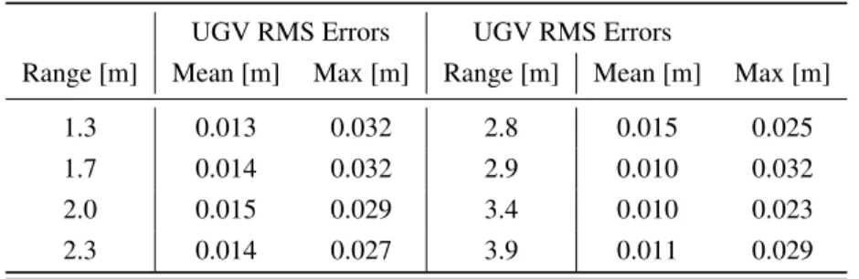
TABLE 3: Magnitude of position errors of the simulated UGV during trials of increasing distance between vehicles.
UGV RMS Errors UGV RMS Errors
Range [m] Mean [m] Max [m] Range [m] Mean [m] Max [m] 1.3 0.013 0.032 2.8 0.015 0.025 1.7 0.014 0.032 2.9 0.010 0.032 2.0 0.015 0.029 3.4 0.010 0.023 2.3 0.014 0.027 3.9 0.011 0.029
TABLE 4: RMSE of vehicles over entire trajectory.
UGV Errors UAV Errors
Ref Dist [m] RMS [cm] RMS [o] Dist [m] RMS [cm] RMS [o]
[2] (Map alignment) 7.7 3.8 - 23 1.2
-[4] (Map alignment) ∼5 7.5 1.5 - -
-[17] (RGB Binocular) - - - 3 12.7 2.0
Experimental 4.1 3.0 0.2 14.7 13 0.2
Simulated 4.1 1.6 0.2 15.2 3.6 0.2
due to the lighting conditions, shading on the edges of the spher-ical markers, and the thresholds applied to convert images from the YUV space to a boolean image. In simulation, detection of the UAV markers fails at an approximate upper limit of 5.25 me-ters. In the laboratory experiments, detection of markers is lim-ited by an upper bound of approximately 5.6 meters. Similarly, the theoretically minimum distance where all three markers are within the FOV of the stereo camera system is 0.45 meters. How-ever, at such close ranges (approximately one body length of the UAV), it is not practical to maintain the UAV within the FOV of the cameras. In practice, an achievable and functional minimum distance for the UAV is approximately 1 meter.
With these limits in mind, we conducted a number of sim-ulated trials for the exploration experiment from Section 4 to provide evidence of the robustness of this methodology to dif-ferent stand-off distances between UAV and UGV while in mo-tion. For 8 different distances within the operational range, we iterated simulated trails of the same configuration as the experi-ments in Section 4. The results of these trials are shown in Table 3. Regardless of distance between vehicles, the error of the po-sition estimate for the UGV remained comparable to the errors reported in the previous section. From these results, we conclude that this methodology is robust enough to successfully localize both vehicles while the UGV navigates to the goal location. This experiment was not attempted in the laboratory due to the space limitations of the motion capture system.
For comparison, the root mean square error (RMSE) of the vehicles in our experiments are listed along side the results of similar experiments in Table 4. For both UGVs and UAVs, the total distance traveled by either UGV or UAV is listed first fol-lowed by the position and orientation errors. The data for the first three rows was collected from the presented results of the cited publications, the bottom two rows of the table correspond to the experimental and simulated results of our work. With re-gard to UGV pose performance, ours are comparable to existing results, with slightly better performance in terms of orientation. For localizing the UAV, the map alignment process from [2] out performed the RGB method presented here, however, the perfor-mance was comparable between our results and those presented in [17].
5 Conclusion
We have presented and evaluated a novel relative localiza-tion scheme for low-cost, heterogeneous, mobile robots with non-overlapping sensing perspectives. An error-state, com-plementary Kalman Filter was developed to fuse analytically-derived uncertainty of stereoscopic pose measurements of an aerial robot, made by a ground robot, with the inertial/visual proprioceptive measurements of the aerial robot. Analysis of simulated and experimental results verified the validity of the er-ror models as well as the ability of the Kalman Filter to track
REFERENCES REFERENCES
the states of both vehicles. The robot team was both simulated and physically developed to test the expected error sources and evaluate the performance in the presence of errors for combined navigation. The effective operation of this team is limited to an approximate inter-robot range between 1 and 5 meters due to the resolution of the cameras equipped by the UGV. This maximum of this range could be increased with more expensive cameras or by lenses with a more narrow field of view, though reducing the field of view would increase the minimum effective limit.
REFERENCES
[1] Fankhauser, P., Bloesch, M., Krsi, P., Diethelm, R., Wer-melinger, M., Schneider, T., Dymczyk, M., Hutter, M., and Siegwart, R., 2016. “Collaborative navigation for fly-ing and walkfly-ing robots”. In Proc. of the IEEE/RSJ In-ternational Conference on Intelligent Robots and Systems (IROS), pp. 2859–2866.
[2] Forster, C., Pizzoli, M., and Scaramuzza, D., 2013. “Air-ground localization and map augmentation using monoc-ular dense reconstruction”. In Proc. of the IEEE/RSJ In-ternational Conference on Intelligent Robots and Systems (IROS), pp. 3971–3978.
[3] Gawel, A., Dub, R., Surmann, H., Nieto, J., Siegwart, R., and Cadena, C., 2017. “3d registration of aerial and ground robots for disaster response: An evaluation of features, de-scriptors, and transformation estimation”. In IEEE Interna-tional Symposium on Safety, Security, and Rescue Robotics (SSRR), pp. 27–34.
[4] Kaslin, R., Fankhauser, P., Stumm, E., Taylor, Z., Mueg-gler, E., Delmerico, J., Scaramuzza, D., Siegwart, R., and Hutter, M., 2016. “Collaborative localization of aerial and ground robots through elevation maps”. In IEEE Interna-tional Symposium on Safety, Security, and Rescue Robotics (SSRR), pp. 284–290.
[5] Oleynikova, H., Burri, M., Lynen, S., and Siegwart, R., 2015. “Real-time visual-inertial localization for aerial and ground robots”. In Proc. of the IEEE/RSJ International Conference on Intelligent Robots and Systems (IROS), pp. 3079–3085.
[6] Piasco, N., Marzat, J., and Sanfourche, M., 2016. “Collab-orative localization and formation flying using distributed stereo-vision”. In Proc. of the IEEE International Confer-ence on Robotics and Automation (ICRA), pp. 1202–1207. [7] Schmuck, P., and Chli, M., 2017. “Multi-uav collaborative monocular slam”. In Proc. of the IEEE International Con-ference on Robotics and Automation (ICRA), pp. 3863– 3870.
[8] Shen, C., Zhang, Y., Li, Z., Gao, F., and Shen, S., 2017. “Collaborative air-ground target searching in complex en-vironments”. In IEEE International Symposium on Safety, Security, and Rescue Robotics (SSRR), pp. 230–237.
[9] Breitenmoser, A., Kneip, L., and Siegwart, R., 2011. “A monocular vision-based system for 6d relative robot local-ization”. In Proc. of the IEEE/RSJ International Conference on Intelligent Robots and Systems (IROS), pp. 79–85. [10] Dewan, A., Mahendran, A., Soni, N., and Krishna, K. M.,
2013. “Heterogeneous ugv-mav exploration using integer programming”. In Proc. of the IEEE/RSJ International Conference on Intelligent Robots and Systems (IROS), pp. 5742–5749.
[11] Dias, D., Ventura, R., Lima, P., and Martinoli, A., 2016. “On-board vision-based 3d relative localization system for multiple quadrotors”. In Proc. of the IEEE Interna-tional Conference on Robotics and Automation (ICRA), pp. 1181–1187.
[12] Faessler, M., Mueggler, E., Schwabe, K., and Scaramuzza, D., 2014. “A monocular pose estimation system based on infrared LEDs”. In Proc. of the IEEE International Confer-ence on Robotics and Automation (ICRA), pp. 907–913. [13] Mueggler, E., Faessler, M., Fontana, F., and Scaramuzza,
D., 2014. “Aerial-guided navigation of a ground robot among movable obstacles”. In 2014 IEEE International Symposium on Safety, Security, and Rescue Robotics (SSRR), pp. 1–8.
[14] Reardon, C., and Fink, J., 2016. “Air-ground robot team surveillance of complex 3d environments”. In IEEE In-ternational Symposium on Safety, Security, and Rescue Robotics (SSRR), pp. 320–327.
[15] Teixeira, L., Maffra, F., Moos, M., and Chli, M., 2018. “Vi-rpe: Visual-inertial relative pose estimation for aerial vehi-cles”. IEEE Robotics and Automation Letters (RAL),3(4), Oct, pp. 2770–2777.
[16] Delmerico, J., Mueggler, E., Nitsch, J., and Scaramuzza, D., 2017. “Active autonomous aerial exploration for ground robot path planning”. IEEE Robotics and Automation Let-ters (RAL),2(2), April, pp. 664–671.
[17] Achtelik, M., Zhang, T., Kuhnlenz, K., and Buss, M., 2009. “Visual tracking and control of a quadcopter us-ing a stereo camera system and inertial sensors”. In In-ternational Conference on Mechatronics and Automation (ICMA), pp. 2863–2869.
[18] Blostein, S. D., and Huang, T. S., 1987. “Error analysis in stereo determination of 3-d point positions”.IEEE Transac-tions on Pattern Analysis and Machine Intelligence, PAMI-9(6), Nov, pp. 752–765.
[19] Matthies, L., and Shafer, S., 1987. “Error modeling in stereo navigation”. IEEE Journal of Robotics and Automa-tion,,3(3), pp. 239–248.
[20] Farrell, J., 2008. Aided Navigation: GPS with High Rate Sensors. McGraw-Hill Education.
[21] Higgins, W. T., 1975. “A comparison of complementary and kalman filtering”. IEEE Transactions on Aerospace and Electronic Systems,AES-11(3), May, pp. 321–325.
REFERENCES REFERENCES
[22] Roumeliotis, S. I., Sukhatme, G. S., and Bekey, G. A., 1999. “Circumventing dynamic modeling: evaluation of the error-state Kalman Filter applied to mobile robot local-ization”. In Proc. of the IEEE International Conference on Robotics and Automation (ICRA), Vol. 2, pp. 1656–1663. [23] Bouabdallah, S., and Siegwart, R., 2005. “Backstepping
and sliding-mode techniques applied to an indoor micro quadrotor”. In Proc. of the IEEE International Conference on Robotics and Automation (ICRA), pp. 2247–2252. [24] Dentler, J., Kannan, S., Mendez, M. A. O., and Voos,
H., 2016. “A real-time model predictive position control with collision avoidance for commercial low-cost quadro-tors”. In IEEE Conference on Control Applications (CCA), pp. 519–525.
[25] Bristeau, P.-J., Callou, F., Vissiere, D., and Petit, N., 2011. “The navigation and control technology inside the AR.Drone micro UAV”. In IFAC world congress, Vol. 18, pp. 1477–1484.
[26] Simon fraser autonomylab. https://github.com/
AutonomyLab/ardrone_autonomy.
[27] Hammer, P., Cappelleri, D., and Zavlanos, M., 2012. Tor-toisebot: Low-cost ros-based mobile 3d mapping platform. Technical Report 1, Stevens Institute of Technology, Hobo-ken, NJ.
[28] Olson, E., 2011. “Apriltag: A robust and flexible visual fiducial system”. In Proc. of the IEEE International Confer-ence on Robotics and Automation (ICRA), pp. 3400–3407. [29] April robotics laboratory at the university of michigan.
https://april.eecs.umich.edu/software/