ABSTRACT
Rock brittleness is one of the important properties for fracability evaluation and can be represented by different physical properties. The mineralogy-based brittleness index (BIM)
builds a simple relationship between mineralogy and brittleness, but it may be ambiguous for rocks with complex micro-structure; while the elastic moduli-based brittleness index (BIE) is
applicable in the field, but BIE interpretation needs to be constrained by lithofacies information.
We propose a new workflow for quantitative seismic interpretation of rock brittleness: lithofacies are defined by a criterion combining both BIM and BIE for comprehensive brittleness
evaluation; statistical rock physics methods are applied for quantitative interpretation by using inverted elastic parameters; acoustic impedance and elastic impedance are selected as the optimized pair of attributes for lithofacies classification. To improve the continuity and accuracy of the interpreted results, Markov random field is applied in the Bayesian rule as the spatial constraint. A 2D synthetic test demonstrates the feasibility of Bayesian classification with Markov random field. This new interpretation framework is also applied to a shale reservoir formation from China. Comparison analysis shows that brittle shale sections can be efficiently discriminated from ductile shale sections and tight sand sections by using the inverted elastic parameters.
Key words: Brittleness, Shale, Statistical rock physics, Markov random field
INTRODUCTION
Unconventional reservoirs of low porosity and permeability need to be hydraulic-fractured to acquire productivity. Rock brittleness is one of the important properties which guides the hydraulic-fracturing. Different properties have been used to represent rock brittleness, and they are generally divided into three categories: (1) hardness and strength; (2) brittle minerals weight fraction; (3) elastic moduli. Hardness and strength analysis provides detailed brittleness properties, but they need to be measured in laboratory experiments (Honda and Sanada, 1956; Hucka and Das, 1974; Altindag and Guney, 2010; Jin et al., 2014; Zhang et al., 2015). The other two categories can be observed by well logging or surface seismic, and thus are more applicable in the field.
A mineralogy-based brittleness index (BIM) was proposed by Jarvie et al. (2007) and Wang
and Gale (2009). Accordingly, rock brittleness is related to quartz content and dolomite content, whereas ductility is related to the content of clay and other minerals. The mineralogy information can be obtained from both core analysis and well-logs. The advantage of a mineralogy-based brittleness index lies in the direct link between the brittleness and lithology, so the brittleness can be determined by a lithological interpretation when the target formation mineralogy is simple. However, besides the mineral content, the presence and distribution of voids and pore fluids may have great influence in rock brittleness (Zhang et al. 2015). Thus, brittleness index analysis using BIM alone cannot be effective, especially for rocks with
complex micro-structure.
Various elastic moduli are used to characterize brittleness. Rickman et al. (2008) proposed an average brittleness index equation of normalized Young’s modulus and normalized Poisson’s ratio according to the two parameters’ different geomechanical effect when fracturing. A high brittleness index corresponds to high Young’s modulus and low Poisson’s ratio. Guo et al. (2012) defined brittleness index by the Lamé parameters of incompressibility and rigidity and explore the effect of fractures and microstructure on rock brittleness based on rock physics modeling. Chen et al. (2014) provided a rock physics modeling framework for brittleness evaluation in terms of the ratio of Young’s modulus and Lamé parameters. Furthermore, different brittleness index measurements were compared in terms of sensitivity and accuracy. Perez et al. (2013) constructed a brittleness template of lamda-rho and mu-rho to interpret seismic inversion results. The advantage of the elastic moduli based BIE index is that it can be
obtained from both well logs and seismic data and thus is more applicable than the mineral-based brittleness index (Rickman et al., 2008). Besides, BIE represents the integrated effects of
mineral content, microstructures and pore fluids in rock brittleness. However, it is difficult to reveal the lithology change by the BIE, because different formations with different lithology
may show similar elastic properties.
We first analyze the relationship between two categories of brittleness indexes (BIM and BIE)
using well logs and effective medium theories. Then we propose a new quantitative seismic interpretation framework of brittleness by integrating BIM and BIE. The lithofacies are defined
parameters of seismic inversion, the statistical rock physics technique in Mukerji et al. (2001) and Avseth et al. (2005) is subsequently applied in the workflow. Since Markov random field and the Markov chain can model the dependencies of vertical and horizontal settings in lithology/fluid prediction (Larsen et al., 2006; Eidsvik et al., 2002) respectively, in this sense, we apply Markov random field as the spatial constraint to improve the continuity and accuracy of the interpreted results. This new interpretation method is demonstrated by application to both synthetic data, and real seismic data of an Upper Triassic shale formation from Sichuan basin, southwest China.
COMPARISON BETWEEN DIFFERENT TYPES OF BRITTLENESS INDEX Rock brittleness is one of the most important properties in reservoir fracturing evaluation, and can be represented by the weight fraction of brittle minerals (Jarvie et al. 2007; Wang and Gale 2009)
_Jarvie(2007) / ( )
M Q Q Ca Cl
BI f f f f (1)
M_Wang(2009) ( Q Dol) / ( Q Dol Ca Cl )
BI f f f f f f TOC (2)
wherefQ, fCa, fCl, fDoland TOC are the weight fractions of quartz, calcite, clay and dolomite, and the total organic carbon content, respectively. Considering the TOC of an in-situ shale
formation, equation (2) is modified as BIM for brittleness evaluation based on the mineralogy
of shale in the study area
M ( Q Carb) / ( Q Carb oth )
BI f f f f f TOC (3)
where fCarband foth are the total weight fractions of carbonate mineral, and weight fractions summation of other minerals expect quartz and carbonates, respectively. The shale mineralogy is shown in Figure 3, and would be further discussed in the following section.
The brittleness index related to pre-failure behavior can also be calculated using the elastic modulus, such as Young’s modulus and Poisson’s ratio (Rickman et al. 2008). Jin et al. (2014) gave a definition of BIE modified from Rickman et al. (2008):
min max max min min max
[ ] / 2 ( ) ( ) E E E BI E E ( ) ( ) (4) where 2 2 2 2 2 4 3 Vs Vp( 3Vs ) E Vp Vs is Young’s modulus, 2 2 2 2 2 2( ) Vp Vs Vp Vs is Poisson’s ratio
,
maxE and Emin are the maximum and minimum value of Young’s modulus in the interval of
interest. maxandminare the maximum and minimum value of Poisson’s ratio in the interval of interest. Vp,Vs and are the P-wave velocity, S-wave velocity and density in the interval of
interest, respectively.
We first analyze the performance of two brittleness indexes in different single mineralogies. Figure 1 shows the brittleness index BIE of 12 common minerals in sedimentary rocks. The
elastic parameters of minerals except kerogen are from Mavko et al. (2003). The elastic parameters of kerogen are reported by Vernik and Landis (1996) and Yan and Han (2017). Brittle minerals, such as quartz and dolomite, tend to show higher BIE than clay. Therefore, BIM
and BIE have similar performance for varied single minerals. Then, we use the real log data to
show the difference between BIM and BIE. The well logs shown in Figure 2 show the logs of
mineral content (clay, organic matters and quartz), P-wave velocity, S-wave velocity, density, Gamma ray, porosity, water saturation and brittleness indexes. The BIM is calculated using
equation (3), while the BIE of rock is calculated using the P-and S-wave velocities and density
based on equation (4). The Voigt-Reuss-Hill average (VRH) model is used to calculate Young’s modulus, Poisson’s ratio and then we can calculate BIE of rock matrix using equation (4). Rock
matrix here includes both mineralogy and organic matters. The formula of the VRH model is shown in Appendix A. There is a good agreement between BIM and BIE of rock matrix, and the
correlation coefficient of them reaches 0.95. However, BIM and BIE of pore-fluid saturated
rocks vary from each other, especially at depths showing high porosity and low water saturation. The correlation coefficient of BIM and BIE of rocks is only 0.66.
QUANTITATIVE SEISMIC INTERPRETATION FOR ROCK BRITTLENESS A new framework for quantitative interpretation
According to the discussion in the previous section, the mineral-based brittleness index and elastic modulus-based brittleness index have their own advantages and disadvantages.
Therefore, integrating BIM with BIE can provide a comprehensive evaluation of rock brittleness.
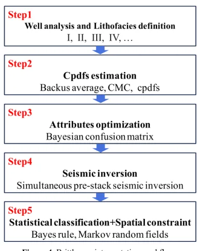
In this sense, we propose a workflow containing the following five steps (Figure 4).
(1) Seismic lithofacies is a seismic-scale sedimentary unit which is characterized by its lithology, bedding configuration, petrography and seismic properties (Avseth et al., 2005). Well logs of mineral content, P-wave velocity, S-wave velocity and density are used as training data to classify the lithofacies related to brittleness based on the crossplot of BIM and BIE. Shale and
sand are classified by BIM threshold, while brittle shale and ductile shale (or brittle sand and
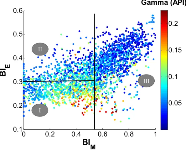
ductile sand) are classified by BIE threshold. As shown in Figure 5, three lithofacies are
classified as: I - ductile shale (low BIM and low BIE), II - brittle shale (low BIM and high BIE),
III – tight sand (high BIM and high BIE). According to the mineralogy of shale core samples
(Figure 3a), the weight fraction of quartz + carbonates is from 42% to 76%, and the average value is 55.01%. Existing studies illustrate that tight-sand formations in the target zone are highly cemented (Gan et al., 2009; Tang et al., 2008), and thus contain generally higher contents of quartz + carbonates than shales. So BIM 55% is set as the threshold for shale-sand
discrimination. Then BIE average value 0.3 is set as the threshold to classify ductile shale and
brittle shale. It might be not necessary to classify ‘brittle sand’ and ‘ductile sand’ in the target zone of this study area, because the tight-sands tend to have high brittleness. Table 1 shows the classification criteria of three lithofacies.
(2) A kernel-based, non-parametric, probability-density estimation is performed to construct the 2-D conditional probability density functions (CPDFs) of training data from well logs, that is the probability distribution p r( | ) of elastic parameter-related attribute (r) values given
lithofacies (Avseth, 2005). The CPDFs are derived by smoothening facies data points in the crossplot space of two different seismic attributes. The Gaussian kernel function is used as the filter template, in which the element at location (i, j) is expressed as
2 2 2 ( 1) ( 1) 2 2
1
( , )
2
i k j kG i j
e
(5) where represents the standard deviation, and the size of template is (2k1)*(2k1).In this step, seismic attributes are calculated from depth-time calibrated well logs (including P-wave velocity, S-wave velocity and density). Well logs are also up-scaled and expanded.
Although Backus average (Backus, 1962) is usually used to calculate the effective elastic constants of vertically transverse isotropic (VTI) medium, it is applied in the workflow to up-scaling the well log data in order to match the seismic data. The effective elastic parameters can be calculated as follows:
1 1 1 1 * ( 2 ) * * Vp Vs , , , (6)
where
,
and
represent Lamé’s parameters, and density, of the thin interbed, respectively. *p
V , *
s
V and
*represent P-wave velocity, S-wave velocity and density of the effective media,respectively. < > represents the weighted average of the enclosed parameters in the length window. The correlated Monte-Carlo (CMC) simulations (Avseth, 2005) are applied to expand
*
p
V , *
s
V and
*for different lithofacies. The up-scaled log of P-wave velocity can be expandedas
* 1( ){ 1, 2,3,... }
i i
Vp F x i N (7) where refers to the th lithofacies,
i
refers to thei
th sampling, F Vp( *) is theprobability cumulative density function of different lithofacies,
x
iis uniform random sample within [0 1], and N is the sample number to be expanded. The corresponding logs of S-wave velocity and density for different lithofacies can then be obtained based on the linear regressions of Vp* and Vs* , and Vp* and ρ*, respectively.(3) The Bayesian rule is used to classify the training data as predicted lithofacies by using different seismic attribute pairs, such as Young’s modulus-Poisson’s ratio and Lamé’s parameters. One optimized seismic attribute pair is selected among them for the target formation of interest. The Bayesian rule is expressed by
argmax( ( | ) ( ))p r p
, (8) where is the estimated classification, r is seismic attributes, corresponds to thelithofacies, p r( | ) is the CPDFs of different lithofacies, and p( ) is the prior probability of
different lithofacies.In this step, p r( | ) corresponding to different seismic attribute pairs can
lithofacies is set as equal to ensure that the estimated classification is completely controlled by
( | )
p r .
In order to verify the classification ability of different attribute pairs, the lithofacies classification of different seismic attribute pairs is used to calculate the Bayesian
classification confusion matrix CM (Avseth et al, 2005; González, 2006), which is expressed as 11 12 1 21 22 2 1 2 n n M n n nn
P
P
P
P
P
P
C
P
P
P
, (9)where the element Pijgives the conditional probability of being
j
th lithofacies given the true lithofaciesi
. Thei
th row of matrix represents the probability of being each lithofacies given thei
th lithofacies. Obviously,1
1
n ij jP
. In particular, the diagonal elements correspond to the success rates of correctly predicting each group.(4) The selected seismic attributes are estimated from prestack seismic data using a simultaneous inversion scheme or an impedance inversion scheme.
(5) In this step, an initial lithofacies classification of the inverted seismic attributes is firstly estimated according to the CPDFs of training data from well logs. Then Markov random field is applied in the estimation of the prior probabilityp( ) , and the most probable lithofacies
classification can be obtained iteratively according to the Bayesian rule shown in equation 8. In each iteration, the prior probability at centre nodes in Markov field is estimated using lithofacies probability of neighbouring nodes from the last iteration, so the final interpretation results can obtain an improvement in spatial and vertical continuity. Markov random field and Markov chain are reviewed in the following subsection.
Markov random field and Markov chain
Markov random field is the generalization of the time-domain Markov chain to the spatial domain (Eidsvik et al., 2002). The basic assumption of the Markov chain can be described as the probability of a lithology-fluid (LF) class to occur at a time t. Given the complete LF
sequence below it, LF at time t depends only on the LF class at the time immediately below, i.e. t+1 (Larsen et al., 2006). The Markov chain model is defined by an upward transition matrix P and the marginal probabilitiesp( )1 , with the elements in P being the transition probabilities
1
( t | t)
p
for all combinations of LF classes. The transition matrix describes the probabilitycharacterization of the Markov process and is independent of time. Because the sequence of sedimentation processes is opposite to the time of seismic data in reservoir geology, it may be natural to define this Markov chain upwards through the geological sequences (Krumbein and Dacey, 1969; Larsen et al., 2006). So the prior probability of LF classes at time t+1 can be calculated as p(
t+1)= ( )*Pp
t . Then p( )
is combined with the conditional probability density function p r( | ) for classifications estimation. The P can introduce the verticalcontinuity of LF into the prior probability p( ) so that the final predicted lithofacies can
be more consistent with geological characterization.
Markov random field is defined as prior distributions for lithofacies under the assumption that the probability distribution of a variable at one location depends on the variable at neighbouring locations. In this study, a second-order neighbourhood system
( )
s
of Markov random field is defined, as indicated in Figure 6. At the centre node s, the probability of each lithofacies is the appearing probability of corresponding lithofacies at the neighbouring nodes, i.e. p(
s| n,sn n,
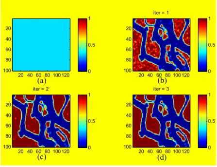
( ))s . Similar as the Markov chain process, this central-node probability is introduced as the prior probability as in equation (8) to restrain the classification process.Markov random field is applied in the Bayesian classification of the Stanford V oilfield model (Mao and Journel, 1999) to verify its advantages in improving lateral continuity. The original lithofacies types and elastic parameters in the model are substituted for the lithofacies I, II, III and their corresponding elastic parameters, while the original spatial correlations of lithofacies are retained. The real lithofacies distribution of oilfield model in time slice is shown in Figure 8a. The prior probability of each lithofacies in the Bayesian classification is equal to 1/(Number of lithofacies) (Figure 7a), and the interpretation result of the Bayesian classification is shown in Figure 8b. Then the central-node probability of all of lithofacies used at the 1st
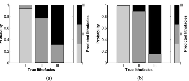
iteration of Markov-random-field-based Bayesian classification is obtained from the initial interpretation result shown in Figure 8b. Figure 7b shows the prior probability of lithofacies I at the 1st iteration. The interpretation results of Markov-random-field-based Bayesian classification of the 1st, the 2nd and the 3rd iteration are shown in Figure 8(c)-8(e), respectively. The central-node probability of each lithofacies used at different iterations are obtained in a similar way as that of the 1st iteration. Figure 7c and 7d show the prior probability of lithofacies I at the 2nd iteration and the 3rd iteration, respectively. The corresponding Bayesian confusion matrix of Bayesian classification without Markov random field and Bayesian classification based on Markov random field are compared in Figure 9. An obvious improvement of lateral continuity can be found when applying Markov random field.
REAL DATA APPLICATION
The study area is in the western Sichuan depression. The target zone is a shale-gas reservoir formation in the Xujiahe Group in the Upper Triassic, T3X5, where T3 refers to the Upper
Group, x refers to the Xujiahe Group, and the superscript indicates the member (Zhang, 2017). Figure 2 showed the well logs through the target formations from 2680m to 3070m depth. T3X5
is placed below the Badaowan Group (J1b), which is an interbedded sandstone-shale facies, and
is typically found deposited on the T3X4, a tick tight sand formation (Gan et al., 2009; Tang et
al., 2008). In addition to clay-rich shales, T3X5 contains several layers of silty shales and sand
intervals of varied thickness. The sand layers show low generally low porosity and permeability, and are similar as those in the deeper sections of the Upper Triassic. The real lithofacies distribution extracted from well-log is compared with P-wave velocity, S-wave velocity, density, synthetic seismic gather and the real seismic gather in the time domain (Figure 10). Based on the brittleness index analysis discussed in step (1), well logs within the target zone are used to classify three lithofacies: I - ductile shale, II - brittle shale, and III – tight sand. BIM
55% is set as the threshold for shale-sand discrimination, and average value of BIE 0.3 is set as
the threshold to classify ductile shale and brittle shale. Most of layers at shallower part can be identified from seismic data, while layers within 1570-1620ms are thin (10ms) and thus may not be fully recovered from seismic data.
The well-log data corresponding to the three lithofacies are depth-time calibrated to construct CPDFs. Figure 11 shows the results of the Backus average and Figure 12 shows the results of correlated Monte-Carlo simulations. The logs of P-and S-wave velocities and density are up-scaled to that of the inverted seismic results with empirical value λ/8 (λ represents the wavelength of seismic data). The number of data points belonging to each facies is expanded to 2000 by using correlated Monte-Carlo simulations. The relationship among elastic parameters needs to be preserved during the data expansion process, if there is strong correlation among them. Linear regressions are found between Vp and Vs of different facies, while the correlation between Vp and density for given facies can be weak (Figure 12). In this sense, data samples of density need to be simulated and expanded individually according to González (2006). Figure 13 shows the histogram of P-wave velocity, S-wave velocity and density for lithofacies I. It is clear that CMC data and the up-scaled well-log data of lithofacies I have a very similar distribution. For lithofacies I, the data points of elastic impedance EI(30o)
and acoustic impedance AI calculated by processed well-log data are compared with their
corresponding CPDFs in Figure 14.
Four pairs of attributes including EI(30o)-AI, Young’s modulus (E)-Poisson’s ratio (v),
lamda (
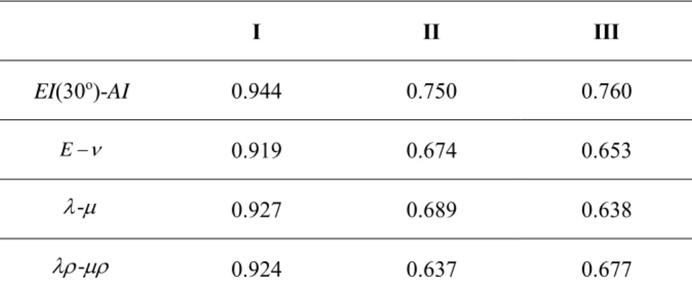
)-mu () (Gray, 2002) and lamdarho ()-murho () (Goodway et al., 1997) are compared in their ability to distinguish between lithofacies. The input data number of every kind of lithofacies is set as equal (2000 points) to balance the database. Figure 15 shows the conditional probability density functions of the four attribute pairs. We calculate the Bayesian classification confusion matrix of these attributes and the probability of correct prediction for each lithofacies is shown in Table 2 and Figure 16. EI-AI shows higher values of probability inthe interpretation of three lithofacies than other three pairs of attributes. The Bayesian confusion matrix corresponding to EI-AI is shown in Table 3 and Figure 17. Each bar in Figure 17
corresponds to a row of the confusion matrix. All of classifications have success rates larger than 75%. So EI-AI is selected as the optimized pair of attributes for the following steps.
Impedance inversion is performed for real seismic data, and it includes the following steps: (1) Transformation of the prestack seismic gathers from the offset domain to the angle domain (Figure 18a and 18b); (2) Seismic data within certain angle intervals are stacked to construct the constant-angle sections (Figure 18c and 18d); (3) Estimation of angle-dependent wavelets
constrained by the investigated well (Figure 18e); (4) Building initial models using the smoothed logs (calibrated in the time domain) and picked horizons; (5) Model-based inversion for both acoustic impedance (AI) and elastic impedance (EI). Steps (3) to (5) are performed by
using the Hampson-Russell software. The final inversion results of seismic attributes EI(30o)
and AI are shown in Figure 19. Although impedance can be more easily regularized than
simultaneous AVO inversion, there might be uncertainties associated with wavelets estimation, initial models or prior information of K (Vp/Vs). Low-pass filtered (0-10Hz) well logs are used to build initial models to guarantee sufficient low frequency components. K is calculated as 0.516 by using original well logs within the target zone. Comparison between synthetic data and real seismic data demonstrates both the inversion results and wavelet estimates (Figure 18c and 18d). However, the small-angle seismic section is noisier than the large-angle seismic section, leading to more patchy AI result. This would also influence the interpretation results. Besides, although most of layers at shallow part can be identified from seismic data, thin layers (e.g tight sand within 1570-1620ms) may not be fully recovered because they have thickness beyond the vertical resolution of seismic data.
Finally, lithofacies are predicted based on Bayes rule by using the probability density functions corresponding to different lithofacies and seismic attributes. Figure 20(a) shows the prediction results from inverted attributes by using Bayesian classification. Markov random field is then performed to improve the accuracy of lithofacies prediction. The final classification is shown in Figure 20(b). The prediction results at well location are compared with the true lithofacies extracted from well logs (Figure 21). Conventional Bayesian classification seems to be patchy due to the influence of seismic noise. Sudden change from tight sand to brittle shale can be seen in many places. Besides, the results at well location (CDP 1396) have little influence in their neighbourhood due to lack of lateral coupling. In contrary, the lithofacies prediction constrained by Markov random field is better reproduced at well location. We evaluate the results from different methods by comparing both with real lithofacies distribution extracted from well-log. There are 290 samples (1396-1685ms) to be classified at the well location. Conventional Bayesian method successfully classifies 170 samples, while the Markov-random-field-based method improves the number from 170 to 193.The result also has much higher horizontal dependence than that of conventional Bayesian classification, and thus
more geologically realistic. Even though, several thin layers are not identified from the prediction because their thickness is beyond the vertical resolution of seismic data.
DISCUSSIONS
Integrating the mineralogy-based brittleness index and elastic moduli-based brittleness index can provide a comprehensive evaluation of rock brittleness. A large number of investigations show that there is difference between static and dynamic elastic properties, and the static-dynamic relation can be varied with rock microstructures, inelastic deformation, experiment equipment and method, loading stage, confining pressure et al. (Simmons and Brace, 1965; Chen and Johnston, 1981; Mavko; 2009; Meléndez-Martínez and Schmitt, 2016;). So brittleness characterization using static elastic moduli estimated from dynamic elastic moduli needs to be investigated in further study. In fact, the difference between dynamic and static elastic moduli decreases with the increase confining pressure (Asef and Najibi, 2013; Meléndez-Martínez and Schmitt, 2016). Meléndez-Martínez and Schmitt (2016) also demonstrated that static elastic moduli in horizontal direction is insensitive to stress and has much higher similarity as dynamic elastic moduli than that in vertical direction. Therefore, considering anisotropy and depth trend (pressure) can also improve the accuracy of static brittleness prediction.
In the interpretation workflow, Backus averaging is an essential procedure for log-data up-scaling. Note that it is only applied to up-scaling the vertical P- and S-wave velocities, and bulk density. In this study, the effect of intrinsic anisotropy of shale is not included in the brittleness evaluation. This could be appropriate because only logs of a vertical well and seismic inversion results from limited angle are used for interpretation. In fact, published investigation shows that this clay- and organic-rich shale formation shows strongly VTI properties (Zhang, 2017), and elastic parameters related to brittleness index (e.g. Young’s modulus and Poison’s ratio) can be largely influenced by anisotropy (Sone and Zoback, 2013; Wang et al., 2015; Gong et al., 2017). So brittleness characterization using Young’s modulus and Poison’s ratio of different directions can be helpful in the development of shale-gas reservoir, and need to be further investigated in future study. Besides, including anisotropy into EI inversion may improve both inversion and interpretation.
The smectite-illite transition is common in shales and is important in brittle characterization. Due to its temperature dependency, there should be depth trend for smectite-illite transition, and also for brittle shale – ductile shale transformation. But in this study, the effect of smectite-illite transition is not involved into the workflow because of the following two reasons: (1) logs of volumetric/weight fractions of constituent clay minerals are not available; (2) mineralogy of shale core samples show that weight fractions of constituent clay mineral are nearly identical (Figure 3b) within the depth interval of target zone. We agree that the smectite-illite transition could be used in the Markov Chain process and worth to be further developed in future study.
CONCLUSIONS
A new seismic interpretation workflow based on statistical rock physics is proposed to enable the quantitative prediction of brittle reservoir formation.The mineralogy brittleness index and elastic brittleness index are combined to provide a comprehensive evaluation of rock brittleness.
EI-AI is selected as the optimized pair of attributes to classify three lithofacies (ductile shale,
brittle shale and tight sand). Markov random field is applied to maintain the spatial continuity of the lithofacies classification. Both synthetic test and real data application demonstrate the feasibility of this method. This new workflow can be used for characterization of unconventional reservoirs requiring hydraulic fracturing.
APPENDIX A. VOIGT AND REUSS BOUNDS
The Voigt upper bound of the effective elastic modulus,
M
V , of a mixture of N phases is 1 N V i i i M f M , (A-1) where the volume fraction of thei
th constituentf
i and the elastic modulus of thei
th constituentM
i.The Reuss lower bound of the effective elastic modulus,M
R, is1
1
N i i R if
M
M
. (A-2)2
V R
VRH
M
M
M
. (A-3) Mathematically, theM
in the Voigt and Reuss formulas makes most sense by computing onlythe shear modulus
and the bulk modulusK
, and then Young’s modulusE
and Poisson’sratio can be calculated using the rules of isotropic linear elasticity.
REFERENCES
Altindag, R., and A. Guney, 2010, Predicting the relationships between brittleness and mechanical properties (UCS, TS, and SH) of rocks: Scientific Research and Essays, 5, 2107– 2118.
Asef, M. R., and A. R. Najibi, 2013, The effect of confining pressure on elastic wave velocities and dynamic to static Young’s modulus ratio: Geophysics, 78, D135-D142.
Avseth, P., T. Mukerji, and G. Mavko, 2005, Quantitative Seismic Interpretation: Cambridge University Press.
Backus, G. E., 1962, Long-wave elastic anisotropy produced by horizontal layering: Journal of Geophysical Research, 67, 4427–4440.
Bandyopadhyay, K., 2009, Seismic anisotropy: geological causes and its implications to reservoir geophysics: Dissertations & Theses - Gradworks.
Berryman, J.G., 1995, Mixture theories for rock properties, in A Handbook of Physical Constants. T.J. Ahrens, ed. American Geophysical Union, Washington. D.C., 205-208.
Cheng, C. H., and M. D. Johnston, 1981, Dynamic and static moduli: Geophysical Research Letters, 8, 39-42.
Chen, J. J., G. Z. Zhang, H. Z. Chen, and X. Y. Yin, 2014, The construction of shale rock physics effective model and prediction of rock brittleness: 84th Annual International Meeting, SEG, Expanded Abstracts, 2861-2865.
Eidsvik, J., H. Omre, T. Mukerji, G. Mavko, P. Avseth, and N. Hydro, 2002, Seismic reservoir prediction using Bayesian integration of rock physics and Markov random fields: A North Sea example: The Leading Edge, 21, no. 3, 290-294.
gas reservoir characterization: Journal of Geophysics and Engineering, 6, 21-28.
Gong, F. B. Di, J. Wei, P. Ding, and D. Shuai, 2018, Dynamic mechanical properties and anisotropy of synthetic shales with different clay minerals under confining pressure: Geophysical Journal International, 212, 2003–2015.
González, E. F., 2006, Physical and quantitative interpretation of seismic attributes for rocks and fluids identification: Stanford University.
Goodway, B., T. Chen, and J. Downton, 1997, Improved AVO fluid detection and lithology discrimination using Lamé parameters λρ, μρ, and λμ fluid stack from P- and S-inversion: 67th Annual International Meeting, SEG, Expanded Abstracts, 183–186.
Gray, D., 2002, Elastic inversion for Lamé parameters: 72th Annual International Meeting, SEG, Expanded Abstracts, 213-216.
Grieser, B., and J. Bray, 2007, Identification of production potential in unconventional reservoirs: SPE Production and Operations Symposium, 106623.
Guo, Z.Q., M. Chapman, and X. Y. Li, 2012, Exploring the effect of fractures and microstructure on brittleness index in the Barnet Shale: 82nd Annual International Meeting, SEG, Expanded Abstract, 1-5.
Honda, H., and Y. Sanada, 1956, Hardness of coal: Fuel, 35, 451–461.
Hucka, V., and B. Das, 1974, Brittleness Determination of Rocks by Different Methods: International Journal of Rock Mechanics & Mining Sciences & Geomechanics Abstracts, 11, no. 10, 389-392.
Jarvie, D. M., R. J. Hill, T. E. Ruble, and R. M. Pollastro, 2007, Unconventional Shale-Gas Systems: The Mississippian Barnett Shale of North-Central Texas as One Model for Thermogenic Shale-Gas Assessment: AAPG Bulletin, 91, no. 4, 475–499.
Jin, X., S. N. Shah, Roegiers J. C., and B. Zhang, 2014, Fracability Evaluation in Shale Reservoirs - An Integrated Petrophysics and Geomechanics Approach: SPE Journal, 20, no. 3, 518-526.
Krumbein, Y. C., and M. F. Dacey, 1969, Markov chains and embedded Markov chains in geology: Mathematical Geology, 1, 79-96.
Larsen, A. L., M. Ulvmoean, H. Omre, and A. Buland, 2006, Bayesian lithology/fluid prediction and simulation on the basis of a Markov –chain prior model: Geophysics, 71, no.
5, R69-R78.
Lonardelli, I., H. Wenk, and Y. Ren, 2007, Preferred orientation and elastic anisotropy in shales: Geophysics, 72, D33-D40.
Loucks, R. G., R. M. Reed, and S. C. Ruppel, 2007, Morphology, genesis, and distribution of nanometer scale pores in siliceous mudstones of the mississipian Barnett Shale: Journal of Sedimentary Research, 79, no. 12, 848-861.
Mao, S., and A. Journel, 1999, Generation of a reference petrophysical/ seismic data set: the Stanford V reservoir: 12th Annual Report, Stanford Center for Reservoir Forecasting, Stanford University.
Mavko, G., T. Mukerji, and J. Dvorkin, 2003, The Rock Physics Handbook: Tool for Seismic Analysis in Porous Media.
Meléndez-Martínez, J., and D. R. Schmitt, 2016, A comparative study of the anisotropic dynamic and static elastic moduli of unconventional reservoir shales: Implication for geomechanical investigations: Geophysics, 81, D245-D261.
Mukerji, T., P. Avseth, G. Mavko, I. Takahashi, and E. F. González, 2001, Statistical rock physics: Combining rock physics, information theory, and geostatistics to reduce uncertainty in seismic reservoir characterization: The Leading Edge, 20, no. 3, 313-319.
Perez, R., and K. Marfurt, 2013, Brittleness estimation from seismic measurements in unconventional reservoirs: Application to the Barnett Shale: SEG Technical Program, Expanded Abstracts, 2258-2263.
Rickman, R., M. J. Mullen, J. E. Petre, W. V. Grieser, and D. Kundert, 2008, A Practical Use of Shale Petrophysics for Stimulation Design Optimization: All Shale Plays Are Not Clones of the Barnett Shale: SPE Technical Conference and Exhibition.
Simmons, G., and W. F. Brace, 1965, Comparison of static and dynamic measurements of compressibility of rocks: Journal of Geophysical Research, 70, 5649-5656.
Sone, H., and M. D. Zoback, 2013, Mechanical properties of shale-gas reservoir rocks – Part 1: Static and dynamic elastic properties and anisotropy: Geophysics, 78, D381-D392.
Tang, J., S. Zhang, and X. Li, 2008, PP and PS seismic response from fractured tight gas reservoirs: A case study: Journal of Geophysics and Engineering, 5, 92-102.
Hydrocarbon Generation and Primary Migration: AAPG Bulletin, 80, no. 4, 531-544. Wang, F., and J. Gale, 2009, Screening Criteria for Shale-Gas Systems: Gulf Coast Association
of Geological Societies Transactions, 59, 779–793.
Wang, Q., Y. Wang, S. Guo, Z. Xing, and Z. Liu, 2015, The effect of shale properties on the anisotropic brittleness criterion index from laboratory study: Journal of Geophysics and Engineering, 12, 866-874.
Zhang, B., T. Zhao, Jin X, and K. J. Marfurt,2015, Brittleness evaluation of resource plays by integrating petrophysical and seismic data analysis: Interpretation, 3, no. 2, T81-T92. Zhang, F., 2017, Estimation of anisotropy parameters for shales based on an improved rock
Figure captions Figure 1. Brittleness index (BIE) of different minerals.
Figure 2. Well logs of clay (black), quartz (grey) weight fraction and TOC (yellow), P-wave velocity, S-wave velocity, density, Gamma ray, porosity, water saturation and brittleness indexes, from left to right.
Figure 3. (a) The mineralogy of 17 shale core samples. (b) The clay composition of shale core samples.
Figure 4. Brittleness interpretation workflow.
Figure 5. Lithofacies definition based on the BIM-BIE crossplot.
Figure 6. Second-order neighbourhood system with centre node (black) and neighbouring nodes (grey).
Figure 7. Prior probability of lithofacies I used in (a) Bayesian classificaiton without Markov random fields, (b) Markov-random-field-based Bayesian classification at the 1st iteration, (c) Markov random based Bayesian classification the 2nd iteration, (d) Markov random field-based Bayesian classification at the 3rd iteration.
Figure 8. (a) Real lithofacies distribution of oilfield model in time slice. (b) Interpretation resu of Bayesian classification without Markov random field. Interpretation results of Markov-random-field-based Bayesian classification of (c) the 1st iteration, (d) the 2nd iteration, and (e) the 3rd iteration.
Figure 9. Bayesian confusion matrix of (a) Bayesian classification without Markov random fields and (b) Markov random field-based Bayesian classification.
Figure 10. (a) Lithofacies distribution extracted from up-scaled well logs: ductile shale (light grey), brittle shale (dark grey), and tight sand (black). Up-scaled well logs of (b) P-wave velocity, (c) S-wave velocity, and (d) density. (e) Stacked seismic trace at well location - CDP 1396 (multiple for display).
Figure 11. Backus average results (red line) and original well logs (black line).
Figure 12. Comparison between CMC results (grey points) and original well-log data (black points): (a) Vp-Vs of facies I, (b) Vp-Density of facies I, (c) Vp-Vs of facies II, (d) Vp-Density of facies II, (e) Vp-Vs of facies III, and (f) Vp-Density of facies III.
Figure 13. Histogram of the real well logs (black) and the CMC results (grey) for facies I: (a) P-wave velocity, (b) S-wave velocity and (c) density.
Figure 14. EI-AI plot for lithofacies I. light-grey points are training data, dark-grey contour represents the corresponding conditional probability density function.
Figure 15. Probability density functions of lithofacises corresponding to different pairs of attributes: (a)EIAI, (b) E (c) - and (d) - .
Figure 16. Bar-graph display of the conditional probability values in Table 2. Figure 17. Bayesian confusion matrix in vertical bars for EI(30 o)-AI.
Figure 18. (a) The common-image-point gather at offset domain (CDP 1396). (b) The common-image-point gather at angle domain (CDP 1396). (c) Constant-angle section of 0 o. (d)
Constant-angle section of 30 o. (e) Estimated wavelets for constant-angle sections 0 o and 30o.
Figure 19. Inversion results of (a) AI (km/s*g/cm3) and (b) EI (km/s*g/cm3). (c) Comparison
between the inverted AI (red) with initial model (black) and well log (blue), synthetic trace (10o)
and seismic trace (10o), from left to right. (d) Comparison between the inverted EI(30o) (red)
with initial model (black) and well log (blue), synthetic trace (30o) and seismic trace (30o), from
left to right.
Figure 20. (a) Interpretation result obtained from Bayesian classification without Markov random field and (b) interpretation result obtained from Bayesian classification based on Markov random field.
Figure 21. (a) Real lithofacies distribution extracted from well-log, (b) Bayesian classification without Markov random field predicted from inversion result at well location and (c) Markov random field-based Bayesian classification predicted from inversion result at the well location.
Lithofacies Criteria
BIM BIE
I <0.55 <0.3
II <0.55 >0.3
III >0.55
Table 1. Classification criteria of three lithofacies based on brittleness index.
I II III EI(30o)-AI 0.944 0.750 0.760 E 0.919 0.674 0.653 - 0.927 0.689 0.638 - 0.924 0.637 0.677
Table 2. The conditional probability of the real lithofacies given the correct prediction of lithofacies (diagonal elements of the Bayesian confusion matrix) for the three pairs of attributes.
True lithofacies
I II III
I 0.944 0.056 0
II 0.038 0.750 0.212
III 0.002 0.238 0.760
Figure 1. Brittleness index (BIE) of different minerals. 0 0.2 0.4 0.6 0.8 1 B rit tle n es s inde x B I E Pyrit e Quart z Fluor apa tite Dolom ite Calc ite Vern ik,s k eroge n Yan ,s ker ogen (ma x) Yan ,s ke roge n (m in) Anor those Feld spar Han ,s cla y Tosa ya ,s cla y 0.862 0.652 0.334 0.288 0.194 0.176 0.121 0.118 0.110 0.106 0.052 0.024
Figure 2. Well logs of clay (black), quartz (grey) weight fraction and TOC (yellow), P-wave velocity, S-wave velocity, density, Gamma ray, porosity, water saturation and brittleness indexes, from left to right.
0 50 100 2920 2940 2960 2980 3000 3020 3040 3060 Mineral wt(%) D ept h (m )
Clay TOC Quartz+Carbonate 2 4 6 Vp (km/s) 1 2 3 4 Vs (km/s) 2 2.5 3 Density (g/cm3) 50 100 150 GR (API) 0 10 2030 Porosity (%) 0 50 100 SW (%) 0 0.5 1 Brittleness index BI M BIE (matrix) BIE (rock)
(a)
(b)
Figure 3. (a) The mineralogy of 17 shale core samples. (b) The clay composition of shale core samples. 0 10 20 30 40 50 60 70 80 Clay Qtz+C b Felds par Arag onite Side rite Augi te
Pyrite Barite
We ig ht f ra ct ion ( % ) 0 10 20 30 40 50 60 I/S Illite Kaolin ite Chlo rite Weight fr action (%)
Figure 4. Brittleness interpretation workflow.
Step1
Well analysis and Lithofacies definition
I, II, III, IV, …
Step2
Cpdfs estimation
Backus average, CMC, cpdfs
Step3
Attributes optimization
Bayesian confusion matrix
Step4
Seismic inversion
Simultaneous pre-stack seismic inversion
Step5
Statistical classification+Spatial constraint
Bayes rule, Markov random fields
Figure 5. Lithofacies definition based on the BIM-BIE crossplot.
0
0.2
0.4
0.6
0.8
1
0.1
0.2
0.3
0.4
0.5
0.6
BI
M
BI
E
Gamma (API)
0.05
0.1
0.15
0.2
I
II
III
Figure 6. Second-order neighbourhood system with centre node (black) and neighbouring nodes (grey).
The probability distribution at the center node depends on the variables at the eight neighboring nodes
Figure 7. Prior probability of lithofacies I used in (a) Bayesian classificaiton without Markov random fields, (b) Markov-random-field-based Bayesian classification at the 1st iteration, (c) Markov random based Bayesian classification the 2nd iteration, (d) Markov random field-based Bayesian classification at the 3rd iteration.
20 40 60 80 100 120 20 40 60 80 100 iter = 1 20 40 60 80 100 120 20 40 60 80 100 iter = 2 20 40 60 80 100 120 20 40 60 80 100 iter = 3 20 40 60 80 100 120 20 40 60 80 100 0 0.5 1 0 0.5 1 0 0.5 1 0 0.5 1 (a) (b) (c) (d)
(a) (b)
(c) (d)
(e)
Figure 8. (a) Real lithofacies distribution of oilfield model in time slice. (b) Interpretation resu of Bayesian classification without Markov random field. Interpretation results of Markov-random-field-based Bayesian classification of (c) the 1st iteration, (d) the 2nd iteration, and (e) the 3rd iteration. 20 40 60 80 100 120 20 40 60 80 100 20 40 60 80 100 120 20 40 60 80 100 20 40 60 80 100 120 10 20 30 40 50 60 70 80 90 100 20 40 60 80 100 120 10 20 30 40 50 60 70 80 90 100 20 40 60 80 100 120 20 40 60 80 100 I II III
(a) (b)
Figure 9. Bayesian confusion matrix of (a) Bayesian classification without Markov random fields and (b) Markov random field-based Bayesian classification.
I II III 0 0.2 0.4 0.6 0.8 1 True lithofacies P ro b ab ility P re d ict ed lit h o fa cie s I II III I II III 0 0.2 0.4 0.6 0.8 1 True lithofacies P ro b ab ility P re d ict ed lit h o fa cie s I II III
(a) (b) (c) (d) (e)
Figure 10. (a) Lithofacies distribution extracted from up-scaled well logs: ductile shale (light grey), brittle shale (dark grey), and tight sand (black). Up-scaled well logs of (b) P-wave velocity, (c) S-wave velocity, and (d) density. (e) Stacked seismic trace at well location - CDP 1396 (multiple for display).
1 2 3 1400 1450 1500 1550 1600 1650 Lithofacies Tim e (m s) 3.5 4 4.5 5 Vp (km/s) 1.5 2 2.5 3 Vs (km/s) 2.4 2.6 Density (g/cm3) CDP 1396
Figure 11. Backus average results (red line) and original well logs (black line). 3 4 5 6 1400 1450 1500 1550 1600 1650 Vp (km/s) Ti me (ms)
Well-log Backus average 1 2 3
Vs (km/s)
2.4 2.6
(a) (b)
(c) (d)
(e) (f)
Figure 12. Comparison between CMC results (grey points) and original well-log data (black points): (a) Vp-Vs of facies I, (b) Vp-Density of facies I, (c) Vp-Vs of facies II, (d) Vp-Density of facies II, (e) Vp-Vs of facies III, and (f) Vp-Density of facies III.
(a) (b)
(c)
Figure 13. Histogram of the real well logs (black) and the CMC results (grey) for facies I: (a) P-wave velocity, (b) S-wave velocity and (c) density.
2 3 4 5 0 0.1 0.2 0.3 0.4
Vp (km/s)
CMC data Raw data 1 1.5 2 2.5 0 0.1 0.2 0.3 0.4Vs (km/s)
CMC data Raw data 2 2.2 2.4 2.6 2.8 0 0.1 0.2 0.3 0.4Density (g/cm
3)
CMC data Raw dataFigure 14. EI-AI plot for lithofacies I. light-grey points are training data, dark-grey contour represents the corresponding conditional probability density function.
(a) (b)
(c) (d)
Figure 15. Probability density functions of lithofacises corresponding to different pairs of attributes: (a)EIAI, (b) E (c) - and (d) - .
(
EI -30° km/s*g/cm
3)
A
I (k
m
/s
*g
/c
m
3)
6 7 8 9 8 10 12 14 I II IIIE (GPa)
20 40 60 0.2 0.25 0.3 0.35 0.4 I II III (GPa)
(
G
P
a)
10 15 20 25 30 5 10 15 20 25 30 I II III *
(GPa*g/cm
3)
*
(
G
P
a*
g
/cm
3)
40 60 80 20 40 60 I II III
Figure 16. Bar-graph display of the conditional probability values in Table 2.
AIEI E 0 0.2 0.4 0.6 0.8 1 P ro b ab ili ty ( T ru e p red ic ti o n ) I II III
Figure 17. Bayesian confusion matrix in vertical bars for EI(30 o)-AI.
I II III 0 0.2 0.4 0.6 0.8 1 True lithofacies P ro b ab ilit y P re d ic te d li th o fac ie s I II III
(a) (b)
(c)
(e)
Figure 18. (a) The common-image-point gather at offset domain (CDP 1396). (b) The common-image-point gather at angle domain (CDP 1396). (c) Constant-angle section of 0 o. (d)
(a) (b) (c) CDP T ime (ms) 1200 1300 1400 1500 1600 1300 1400 1500 1600 1700 1800 1900 AI (km/s*g/cm3) 8 9 10 11 12 13 CDP T ime (ms) 1200 1300 1400 1500 1600 1300 1400 1500 1600 1700 1800 1900 EI-30° (km/s*g/cm3) 6 6.5 7 7.5 8 8.5 10 15 1400 1450 1500 1550 1600 1650 AI (km/s*g/cm3) Time (ms) Original Log Inital Model Inversion Result
(d)
Figure 19. Inversion results of (a) AI (km/s*g/cm3) and (b) EI (km/s*g/cm3). (c) Comparison
between the inverted AI (red) with initial model (black) and well log (blue), synthetic trace (10o)
and seismic trace (10o), from left to right. (d) Comparison between the inverted EI(30o) (red)
with initial model (black) and well log (blue), synthetic trace (30o) and seismic trace (30o), from
left to right. 6 7 8 9 1400 1450 1500 1550 1600 1650 EI-30°(km/s*g/cm3) T ime ( ms) Original Log Inital Model Inversion Result
(a)
(b)
Figure 20. (a) Interpretation result obtained from Bayesian classification without Markov random field and (b) interpretation result obtained from Bayesian classification based on Markov random field.
CDP T ime (ms) I II III 1200 1300 1400 1500 1600 1300 1400 1500 1600 1700 1800 1900 Lithofacies CDP T ime (ms) I II III 1200 1300 1400 1500 1600 1300 1400 1500 1600 1700 1800 1900 Lithofacies
(a) (b) (c) Figure 21. (a) Real lithofacies distribution extracted from well-log, (b) Bayesian classification without Markov random field predicted from inversion result at well location and (c) Markov random field-based Bayesian classification predicted from inversion result at the well location.
1 2 3 1400 1450 1500 1550 1600 1650