Scalable Collaborative Targeted Learning for High-dimensional Data

(1)

University of California, Berkeley

U.C. Berkeley Division of Biostatistics Working Paper Series

Year  Paper

Scalable Collaborative Targeted Learning for

Large Scale and High-dimensional Data

Cheng Ju∗ Susan Gruber† Samuel D. Lendle‡

Jessica M. Franklin∗∗ Richard Wyss††

Sebastian Schneeweiss‡‡ Mark J. van der Laan§

∗_{Division of Biostatistics, University of California, Berkeley, [email protected]}

†_{Harvard Pilgrim Health Care Institute and Harvard Medical School, [email protected]} ‡_{Division of Biostatistics, University of California, Berkeley, [email protected]} ∗∗_{Division of Pharmacoepidemiology and Pharmacoeconomics, Department of Medicine,} Brigham and Women’s Hospital and Harvard Medical School

††_{Division of Pharmacoepidemiology and Pharmacoeconomics, Department of Medicine,} Brigham and Women’s Hospital and Harvard Medical School

‡‡_{Division of Pharmacoepidemiology and Pharmacoeconomics, Department of Medicine,} Brigham and Women’s Hospital and Harvard Medical School

§_{Division of Biostatistics, University of California, Berkeley, [email protected]}

This working paper is hosted by The Berkeley Electronic Press (bepress) and may not be commer-cially reproduced without the permission of the copyright holder.

http://biostats.bepress.com/ucbbiostat/paper352 Copyright c2016 by the authors.

(2)

Scalable Collaborative Targeted Learning for

Large Scale and High-dimensional Data

Cheng Ju, Susan Gruber, Samuel D. Lendle, Jessica M. Franklin, Richard Wyss,

Sebastian Schneeweiss, and Mark J. van der Laan

Abstract

<blockquote>The collaborative double robust targeted maximum likelihood es-timator (C-TMLE) is an extension of targeted minimum loss-based eses-timators (TMLE) that pursues an optimal strategy for estimation of the nuisance param-eter. The original implementation of C-TMLE algorithm uses a greedy forward stepwise selection procedure to construct a nested sequence of candidate nuisance parameter estimators. Cross-validation is then used to select the candidate that minimizes bias in the estimate of the target parameter, rather than basing selec-tion on the fit of the nuisance parameter model. C-TMLE has exhibited superior relative performance in analyses of sparse data, but the time complexity of the al-gorithm is $\mathcal{O}(pˆ2)$, where $p$, is the number of covariates available for inclusion in the model. Despite a criterion that allows for early termination, the greedy algorithm does not scale to large scale and high dimensional data. This article introduces two scalable versions of C-TMLE. Each relies on an eas-ily computed data adaptive pre-ordering of the variables. The time complexity of these scalable algorithms is $\mathcal{O}(p)$, and an early data adaptive stop-ping rule further reduces computation time without sacrificing statistical perfor-mance. We also introduce SL-CTMLE, an approach that uses super learning to select the best variable ordering from a set of ordering strategies. Simulation studies illustrate the performance of the scalable C-TMLEs relative to the origi-nal C-TMLE, the augmented inverse probability of treatment weighted estimator (A-IPTW), the probability of treatment weighting (IPTW) estimator, and stan-dard TMLE using an external non-collaborative estimator of the treatment mech-anism. Scalable C-TMLEs were also applied to three real-world health insurance claims datasets to estimate an average treatment effect. High-dimensional co-variates were generated from the claims data based on high-dimensional propen-sity score (hdPS) screening. All C-TMLEs provided similar estimates and mean

(3)

squared errors. Scalable C-TMLE analyses ran ten times faster than the original C-TMLE in larger datasets, making C-TMLE a feasible option for the analysis of large scale high dimensional data. </blockquote>

(4)

1 Introduction

The collaborative double robust targeted maximum likelihood estimator (C-TMLE) is an extension of targeted minimum loss-based estimators (TMLE) that pursues an optimal strategy for estimation of the nuisance parameter. C-TMLE is a general methodology that can be applied to a variety of estimators in many settings, including survival analysis [18], gene association studies [25] ,and longitudinal data structures [17]. The original implementation of C-TMLE algorithm uses a greedy forward stepwise selection procedure to construct a nested sequence of candidate estimators of the nuisance parameter. Cross-validation is then to select the candidate from this set that minimizes bias in the estimate of the target parameter, rather than optimize the fit of the nuisance parameter model. This C-TMLE exhibits superior relative performance in analyses of sparse data, but its time complexity is O(p2), where p is the number of candidate models and is equal to the number of covariates available for adjustment. Despite a criterion for early termination, the algorithm does not scale to large scale and high dimensional data.

In this article we propose two scalable versions of C-TMLE that replace the greedy search at each step by an easily computed data adaptive pre-ordering of the variables. The time complex-ity of each scalable algorithm is _O(p), and an early data adaptive stopping rule further reduces computation time without sacrificing statistical performance. We also introduce SL-CTMLE, an approach that avoids a priori specification of a single pre-ordering by using super learning (SL) to select the best pre-ordering from a set of ordering strategies. The performance of pre-ordered C-TMLEs is compared with some common established estimation methods: G-computation [13], inverse probability of treatment weighting (IPTW) [8, 14], augmented inverse probability of treat-ment weighted estimator (A-IPTW) [11, 12, 15], and unadjusted regression estimation of a point treatment e↵ect.

The paper is organized as follows. Sections 2 and 3 review TMLE and describe the C-TMLE template. Section 4 reviews the greedy C-TMLE algorithm. Section 5 introduces the two proposed pre-ordered scalable C-TMLEs, and SL-CTMLE. Other common estimators of causal e↵ects found in the literature are compared to C-TMLEs through simulation studies in Section 6. In Section 7, we compare the performance of the new C-TMLEs with standard TMLE on three real data-sets. Section 8 presents and compares the empirical processing time for C-TMLEs with di↵erent sample sizes (n) and feature dimension (p). Section 9 provides notes on a package that implements all the proposed C-TMLEs. The paper concludes with a discussion in Section 10.

1.1 Background

Consider the problem of estimation of the average causal treatment e↵ect (ATE) based on an observational study in which we observe on each unit baseline covariates, W, a binary treatment indicator, A, and a binary or continuous outcome of interest, Y. We use Oi = (Wi, Ai, Yi) to

represent the i-th observation from the unknown observation data distribution P0. Assume a non-parametric structural equation model defined by:

W =fW(UW),

A=fA(W, UA),

Y =fY(A, W, UY).

The potential outcome under treatment at level a2 0,1 is obtained by substituting a fixed value forA infY,Ya=fY(W, a, UY).

(5)

We define the propensity score (PS) as the conditional probability receiving treatment, g0 = E(A_|W),and usegn to denote an estimator of g0. We define the conditional outcome density as,

¯

Q0(A, W) =E(Y |A, W),and estimated conditional density ¯Qn(A, W). Our parameter of interest

, , is the average treatment e↵ect (ATE), defined as =E(Y1 Y0).

A causal interpretion of this statistical estimand requires additional identifiability assumptions. We make the randomization assumption, A?(Y1, Y0)|W,which means given baseline covariates, treatment is independent of potential outcomes (no unmeasured confounders). We also assume positivity, 0< P(A= 1_|W)<1 almost everywhere, which means that given a possible realization of baseline covariates, the probability of being assigned treatment at either level is non-zero. Under these identifiability assumptions, we estimate this causal target parameter with the mapping:

(P0) =E0(Y |A= 1) E(Y |A= 0) =E0[E0(Y |A= 1, W) E0(Y |A= 0, W)].

2 Brief Review of Targeted Maximum Likelihood Estimation

Doubly robust (DR) efficient estimators are estimators that solve the efficient influence curve (EIC) equation for the parameter of interest. The EIC, D⇤(O), for the ATE parameter is given by,

D⇤(O) =H(A, W)[Y Q¯(A, W)] + ¯Q(1, W) Q¯(0, W) ,

whereH(A, W) = (A/g(1, W) (1 A)/(g(0, W)). The double robust A-IPTW directly solves this equation to estimate . In contrast, TMLE is a two-step estimation procedure. Step 1 is to obtain an initial outcome regression estimate, ¯Q0

n(A, W). The second step targets this estimate to obtain

an updated estimate, ¯Q⇤_n(A, W). Targeting involves defining a parametric submodel, using the covariate H(A, W) that incorporates a propensity score, ¯Q⇤_n(A, W) = ¯Q0_n(A, W) +✏H(A, W).As a by-product of using maximum likelihood estimation to fit the fluctuation parameter, ✏, the EIC equation is solved. In practice, bounded continuous outcomes and binary outcomes are fluctuated on the logit scale to ensure bounds on the model space are respected [5]. The parameter estimate is calculated by plugging the updated estimated counterfactual outcomes into the G–computation formula for the ATE parameter (so it is also a plug-in estimator):

n= 1 n n X i=1 ¯ Q⇤_n(1, W) Q¯⇤_n(0, W).

Proofs and technical details are available in the literature [24].

3 General Template of Collaborative Targeted Maximum

Likeli-hood Estimation

TMLE uses the nuisance parameter in a targeting step aimed at reducing bias in the estimate of the parameter of interest by reducing the distance between an initial estimator,Qnand the true relevant

density, Q0. The standard TMLE relies on an external estimate of the nuisance parameter. In contrast, C-TMLE constructs a nuisance parameter estimate that maximizes the goodness-of-fit for an updated density estimate,Q⇤_n. Construction of the nuisance parameter estimates by the original implementation of C-TMLE is based on data-adaptive forward stepwise search that improved the goodness-of-fit of the overall density estimate, Qn, and the nuisance parameter estimate, gn, at

(6)

maximizes the cross-validated likelihood. C-TMLE enjoys all the properties of the standard TMLE estimator, namely, it is double robust and asymptotically efficient under appropriate regularity conditions [21]. We review the general template of collaborative targeted maximum likelihood estimation of the additive treatment e↵ect before defining the pre-ordered C-TMLE.

Algorithm 1 General Template of Collaborative Targeted Maximum Likelihood Estimation 1: Construct an initial estimate ¯Q0_n for ¯Q0=E(Y |A, W).

2: Create candidate TMLEs ¯Q⇤_n,k, using a treatment mechanism estimate, such that the empirical fits of ¯Q⇤_n,k (based on the loss function for ¯Q0) are increasing in k, andgn,k are increasing in k.

The standard C-TMLE uses a forward greedy selection algorithm.

3: Select the best candidate ¯Q⇤_n = ¯Q⇤_n,k_n using loss-based cross-validation, with the same loss function as in the TMLE targeting step.

The best candidate is selected based on the coss-validated penalized log-likelihood. The cross validation selector [5, 23] is defined as

kn= arg min k

cvRSS+cvV ark+n⇥cvBias2k

where these terms are given by

cvRSSk = V X V=1 X i2V al(v) (Yi Qˆ¯⇤k(Pnv0 )(Wi, Ai))2, cvV ark = V X V=1 X i2V al(v) D⇤2( ˆQ¯⇤_k(P_nv0 ),ˆgk(Pn),ˆ( ˆQ⇤k(Pnv0 )))(Oi), cvBiask = 1 V V X v=1 ( ˆQ⇤_k(P_nv0 )) ( ˆQ⇤_k(Pn)).

Theory requires that the sequence (gn,k:k) of estimates grow toward and arrive at a consistent

estimate of the trueg0, wherekis the model index. Building nested candidate estimatesgn,k is one

particular approach that satisfies this requirement, and ensures that for allm < k,gn,k is a better

empirical fit for the treatment mechanism thangn,m [23].

4 Initial Implementation of Collaborative Targeted Maximum

Like-lihood Estimation

The original implementation of C-TMLE used a forward selection algorithm to build the sequence of treatment models: At each stepk+ 1, it incorporates a single additional covariate into the model forg. This covariate is selected from the set of covariates inW that have not been selected in steps 1 through k, as follows. One begins with the intercept model for g to construct a first fluctuation covariate,H1(A, W), which is used to create the first targeted maximum likelihood candidate, ¯Q1_n. Set g1_n(1 _|W) = P(A = 1), g_n1(0_| W) = P(A = 0),and H1(A, W) = ⇣ _I_[_A_=1] g1 n(1|W) I[A=0] g1 n(0|W) ⌘ . Then ¯

Q1_n= ¯Q0_n+✏1H1, where✏1 is fitted by a regression of Y on H1 with o↵set ¯Q0n, is the first targeted

(7)

The second candidate TMLE will be based on an updated model for g that contains the intercept and one covariate. Each covariate,Wj, is considered in turn for inclusion in the propensity

score model. H2,j is evaluated and used to obtain a candidate targeted TMLE, ¯Q2n,j. The loss

function, _L, based on a log-likelihood criterion for the targeted MLE fit is evaluated for each candidate update of the current initial estimate ¯Qk

n,j. The candidate that minimimzes the loss is

incorporated into the propensity score model. This forward stepwise process continues until all covariates inW have been incorporated into the model forg. If at any stepk+ 1 the loss increases such that _Lk+1 >Lk, then the parametric submodel used to update the initial ¯Q0n is extended to

include an additional fluctuation covariate.

Once all candidates have been constructed, cross-validation is used to select the optimal number of covariates to include in the propensity score model. When there are p covariates, choosing the first term requirespcomparisons, choosing the second term requiresp 1 comparisons, etc., making the time complexity of this algorithm _O(p2).

Note there are many variations of the forward greedy stepwise C-TMLE estimator. For ex-ample, one may update the initial estimate ¯Q0_n with the final selected clever covariate defined by carrying out the forward selection algorithm to obtain a g-fit. However, these variations did not improve performance in simulation studies [6]. In this article, the greedy C-TMLE is defined by the procedure just described.

5 Scalable Algorithm for Collaborative Targeted Maximum

Like-lihood Estimation

The processing time for the initial implementation of C-TMLE is highly sensitive to the number of covariates p, as it uses a greedy forwards stepwise search. The time complexity for the algorithm with respect to the dimension is_O(p2_{), which is unsatisfactory for large scale and high dimensional} data. For example, the high-dimensional propensity score (hdPS) algorithm is a method to extract information from electronic medical claims data that produces hundreds or even thousands of candidate covariates, increasing the dimension of the data dramatically. [16] In order to apply C-TMLE to large scale and high-dimensional data, we propose two pre-order strategies for C-C-TMLE. To overcome the computation issue, we propose two algorithms for pre-ordering the covariates so that at each step only one covariate is eligible for inclusion in the propensity score model. The logistic ordering andpartial correlation ordering procedures are described next.

5.1 Logistic Ordering

The logistic ordering ranks covariates by evaluating all p univariate propensity score models, and using each to fluctuate ¯Q0_n. The loss function is evaluated for each of theptargeted estimates, and covariates are ordered so that the one that most improves the loss function is at the start of the sequence.

(8)

Algorithm 2 Logistic Ordering 1: foreach covariate Wj inW do

2: Estimate gn,j(Wj) =E(A|Wj).

3: Fit fluctuation parameter✏j by using Hgn,j(A, Wj) to target ¯Q0n.

4: Compute the loss,Lj, using the loss function for ¯Qjn⇤(e.g, negative log-likelihood for discrete

outcome), where ¯Qjn⇤(A, W) = ¯Q0n(A, W) + ˆ✏jHgn,j(A, Wj). 5: end for

6: Rank the covariates based onLj, the corresponding loss for each covariate.

This procedure is exactly the same as the first round search of the greedy C-TMLE. In other words, instead of selecting the first covariate from the first round, the logistic ordering ranks all covariates by their ability to reduce bias.

5.2 Partial Correlation Ordering

Recall that C-TMLE selects covariates for estimating the nuisance parameter that explain the di↵erence between the initial estimator of the conditional density of the outcome, Q0_n, and the true relevant density, Q0. This motivates the partial corrleation ordering. This ordering ranks covariates based on the absolute value of partial correlation between each covariate Wj inW and

the residual of the outcome and the initial estimator,Y Q¯n(A, W), within strata ofA. The most

highly correlated covariate is placed at the start of the sequence.

Formally, the partial correlation between X and Y given a set of n controlling variables Z =

Z1, Z2,· · · , Zn, written ⇢_XY_Z˙, is the correlation between the residuals RX and RY resulting from

the linear regression of X withZ and of Y withZ, respectively [7]. For our purposes the formula simplifies to: ⇢r,Wj·A= ⇢(r, Wj) ⇢(r, A)·⇢(Wj, A) p (1 ⇢(r, A)2₎₍₁ _⇢(_W j, A)2)

where r is the residual and ⇢(x, y) is the correlation of variablesx and y.

Algorithm 3 Partial Correlation Ordering

1: Estimate ¯Q0_n(A, W), based on all covariates W and A. 2: Compute the residualsri= (Yi Q¯0n(Ai, Wi)).

3: foreach covariate Wj inW do

4: Compute the partial correlation ⇢r,Wj·A ofWj and r given A. 5: end for

6: Rank the covariates based on the absolute value of the partial correlation⇢r,Wj·A

Once an ordering over the covariates has been established, at each step the C-TMLE procedure is used only to decide whether or not to make an additional fluctuation to the baseline model for

¯

Q. If use of the larger propensity score model does not improve the empirical likelihood for Q, an additional fluctuation parameter is fit. Cross-validation is used to choose the number of covariates incorporated into the model, by choosing the number of steps that minimizes the cross-validated loss function. For both the greedy C-TMLE and the pre-ordered C-TMLEs, most bias reduction occurs in the early steps of the algorithm, when smaller propensity score models are being considered for the targeting step. Since conditioning on more covariates tends to inflate the variance of the target

(9)

parameter, this behavior will often reduce variance as well, relative to using an external propensity score estimator. However, the time complexity of a pre-ordered C-TMLE is _O(p). Computation time grows linearly with respect to the number of covariatesp, rather than exponentially.

5.3 Super Learning Based Collaborative Targeted Maximum Likelihood Esti-mation

Super Learning based Collaborative Targeted Maximum Likelihood Estimation (SL-CTMLE) is an extension of C-TMLE that simultaneously explores candidate C-TMLEs that rely on di↵erent nuisance parameter estimation strategies. It can be used to select the single best strategy (discrete SL-CTMLE), or an optimal combination (ensemble SL-CTMLE). The Super Learner (SL) is an ensemble machine learning approach that relies on cross-validation. SL has been proven to asymp-totically perform as well as an oracle selector. [22, 20, 19]. SL-CTMLE is a flexible extension of C-TMLE that can include both greedy search and preordering methods. However, it is not scalable if any of the candidate C-TMLE in the library is not scalable (e.g. greedy search). In this paper we focus on a scalable discrete SL-CTMLE that uses cross-validation to choose among candidate pre-ordering C-TMLEs. Thus cross-validation is used to select both the number of covariates included in the propensity score model, and the ordering procedure itself. We compare these preordered C-TMLEs and SL-CTMLE with greedy C-TMLE and other common methods in later sections.

Algorithm 4 Super Learning C-TMLE

1: Input several covariate order strategies for C-TMLE

2: Use the general template of C-TMLE to find best estimator of treatment for clever covariate 3: Use cross-validated loss to select the best candidate C-TMLE

The time complexity of SL-CTMLE is equal to that of the most complex strategy considered. If only pre-ordering strategies that are O(p) are considered, then SL-CTMLE’s time complexity is O(p). Given a constant number of user supplied strategies, SL-CTMLE remains scalable, with a processing time that is approximately equal to the sum of the times for each strategy.

When candidate pre-ordering strategies are a collection of more and less agressive algorithms, cross-validating the pre-ordering itself is recommended. In this situation, SL-CTMLE would begin by dividing the data intoV folds. Each fold, v₂1, . . . , V is considered the validation set in turn, while observations in the remaining folds constitute the training set. Each candidate C-TMLE is fit using data in the training set, and evaluated using observations in the test set. Since each observation is a member of exactly one test set, each makes a single contribution to the calculation of the validated loss. The discrete SL-CTMLE is the candidate that minimizes the cross-validated loss. The actual processing time will be approximatelyV times the sum of the individual processing times.

6 Simulation

We carried out three Monte Carlo simulation studies to investigate the performance of the scalable C-TMLEs, greedy C-TMLE, G-computation, IPTW, and A-IPTW estimators in estimating the ATE parameter. N = 1000 Monte Carlo data sets of sizen= 1000 were generated for each study. Propensity score estimates were truncated to fall within the range [0.025,0.975] for all estimators.

(10)

The estimators are defined as follows: unadj n = Pn i=1I(Ai = 1)Yi Pn i=1I(Ai = 1) Pn i=1I(Ai = 0)Yi Pn i=1I(Ai = 0) , Gcomp n = 1 n n X i=1 (Q0_n(1, Wi) Q0n(0, Wi)), IP T W n = 1 n n X i=1 [I(Ai = 1) I(Ai= 0)] Yi gn(Ai, Wi) , A IP T W n = 1 n n X i=1 [I(Ai = 1) I(Ai = 0)] gn(Ai |Wi) (Yi Q0n(Wi, Ai)) +1 n n X i=1 (Q0_n(1, Wi) Q0n(0, Wi)), C T M LE n = T M LEn = 1 n n X i=1 (Q⇤_n(1, Wi) Q⇤n(0, Wi)).

6.1 Simulation 1: Low dimensional highly correlated data

In the first simulation study, data were simulated based on a data generating distribution published by Freedman and Berk [3] and further analyzed by Petersen at el. [10]. Two multivariate normal baseline covariates,W1, W2, are generated as,

(W1, W2)⇠N(µ,⌃) where µ1= 0.5, µ2= 1 and ⌃=



2 1 1 1 The propensity score is given by,

P0(A= 1|W) =g0(1|W) =logit 1(0.5 + 0.25W1+ 0.75W2)

This is a slight modification of the mechanism in the original paper, which used a probit model to generate treatment. The outcome is continous, with

¯

Q0(A, W) =E(Y |A, W) = 1 +A+W1+ 2W2, and

Y = ¯Q0(A, W) +✏, with✏⇠N(0,1).

The true value of the target parameter, 0 = 1. The two baseline covariates are highly corre-lated. With this treatment mechanism g 2 [0,1], resulting in practical violation of the positivity assumption.

Each of the four estimators was implemented two ways: 1. using a correctly specified model to estimate both Q0 and g0. 2. using a correctly specified model to estimate g0, and a misspecified model to estimate ¯Q0 (obtained by regressingY on A and W1). We use the linear regression to fit theQ model and logistic regression to fit the treatment model. Propensity scores incorporated into IPTW, A-IPTW, and TMLE were based on the full treatment model forg0.

(11)

Table 1: Simulation study 1. Performance of estimators in 1000 simulated data sets of size 1000.

correct Q¯ misspecified Q¯

bias se MSE bias se MSE

Unadj 2.7668 0.2261 7.7063 2.7668 0.2261 7.7063 A IPTW 0.0007 0.0954 0.0091 0.0108 0.1352 0.0184 IPTW 0.0759 0.3491 0.1275 0.0759 0.3491 0.1275 MLE 0.0010 0.0820 0.0067 0.6994 0.1396 0.5086 TMLE 0.0006 0.0955 0.0091 0.0013 0.1105 0.0122 greedy C-TMLE 0.0008 0.0891 0.0079 0.0004 0.1041 0.0108 logRank C-TMLE 0.0001 0.0894 0.0080 0.0004 0.1041 0.0108 partRank C-TMLE 0.0003 0.0894 0.0080 0.0004 0.1041 0.0108 SL-CTMLE 0.0001 0.0907 0.0082 0.0004 0.1041 0.0108

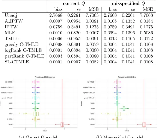
(a) Correct Q model (b) Misspecified Q model

Figure 1: Simulation 1: Box-plot of estimations for ATE with correct/misspecified Q model Bias, variance, and mean squared error (MSE) for all estimators across 1000 simulated datasets are shown in Table 1. Box-plots of the estimated treatment e↵ects are shown in Fig. 1. When Q

was correctly specified, all models had very small bias. IPTW does not use information in the Q

portion of the likelihood. As Freedman and Berk discussed, even when the correct propensity score model is used, near positivity violations can lead to finite sample bias for IPTW estimators (see also [10]). Scalable C-TMLEs had smaller bias than the other DR estimators, but the distinctions were small.

WhenQwas not correctly specified the MLE estimator was expected to be biased. Interestingly, A-IPTW was more biased than the other DR estimators when Q was misspecified. All C-TMLEs have identical performance, because each approach produced the same treatment model sequence. 6.2 Simulation study 2: Highly correlated covariates

W1, W2, W3 iid⇠Bernoulli(0.5)

W4 ⇠Bernoulli(0.2 + 0.5·W1)

W5⇠Bernoulli(0.05 + 0.3·W1+ 0.1·W2+ 0.05·W3+ 0.4·W4)

W6 ⇠Bernoulli(0.2 + 0.6·W5)

(12)

W8⇠Bernoulli(0.1 + 0.2·W2+ 0.3·W6+ 0.1·W7)

P0(A= 1|W) =g0(1|W) =logit 1( 0.05+0.1·W1+0.2·W2+0.2·W3 0.02·W4 0.6·W5 0.2·W6 0.1·W7)

Y = 10 +A+W1+W2+W4+ 2·W6+W7+✏ where ✏_⇠N(0,1)

In this case, the true confounders areW1, W2, W4, W6, W7. Covariates are not independent. W5 is most closely related to W1,W4 . W3 is mainly associated with W7, and a few others. Neither

W3 nor W5 is a confounder: both of them are predictive of treatment A, but not associated with outcomeY. Including either one of them in the propensity score model will inflate the variance [1]. The true ATE for this simulation study is 0 = 1.

Each of the four estimators was implemented in two ways: 1. A correctly specified model was used to estimate ¯Q0, and the correct main terms logistic regression was used to estimate g0, 2. A main terms logistic regression model was used to estimate g0 and a misspecified model was used to estimate ¯Q0 (unadjusted regression of Y on A). Propensity scores incorporated into IPTW, A-IPTW, and TMLE were based on the full treatment model forg0.

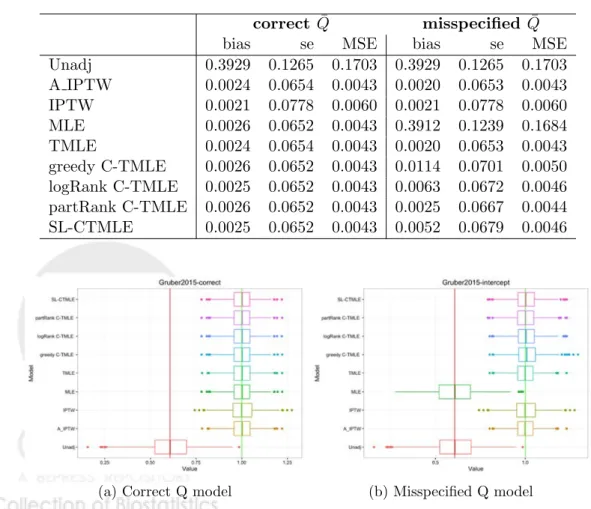
Table 2: Performance of estimators in 1000 simulated data sets of size 1000

(13)

Table 2 demonstrates performance of the estimators across 1000 samples and the box-plots of the estimated treatment e↵ects is shown in Fig. 2. WhenQwas correctly specified, all estimators except the unadjusted estimator had small bias. The DR estimators had lower MSE than the inefficient IPTW estimator. When Q was misspecified the A-IPTW and IPTW estimators were less biased than the C-TMLE’s. The bias of the greedy C-TMLE was five times larger. However, all DR estimators had lower MSE than the IPTW estimator, with TMLE outperforming the others. 6.3 Simulation 3: Binary outcome with instrumental variable

In the third simulation, we assess the performance of C-TMLE in a data set with positivity viola-tions. We first generate W1, W2, W3 ⇠ U

i.i.d.(0,1). A⇠Bernoulli(pA), with

pA=p(A= 1|W) =logit 1( 2 + 5W1+ 2W2+ 1W3) .

OutcomeY ⇠Bernoulli(pY),

pY =P(Y = 1|A, W) =logit 1( 3 + 2W2+ 2W3+W4+A).

Each of the four estimators was implemented in two ways: 1. A correctly specified model was used to estimate ¯Q0, and the correct main terms logistic regression was used to estimateg0, 2. The main terms logistic regression model was used to estimate g0 and a misspecified model was used to estimate ¯Q0 (unadjusted regression of Y on A). Propensity scores incorporated into IPTW, A-IPTW, and TMLE were based on the full treatment model forg0.

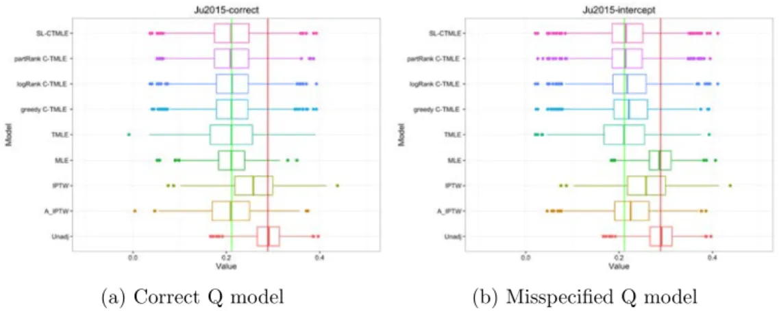
Table 3: Performance of estimators in 1000 simulated data sets of size 10000

(14)

Figure 3: Simulation 3: Box-plot of estimations for ATE with correct/misspecified Q model Table 3 demonstrates performance of the estimators across 1000 samples. Fig. 3 shows box-plots of the estimates for di↵erent methods across 1000 simulation, with a correct/misspecified Q

model.

WhenQwas correctly specified the DR estimators had similar bias/variance tradeo↵s. Although IPTW is a consistent estimator whengis correctly specified, truncation of propensity scoregnmay

have introduced bias. However, without truncation, it will be extremely unstable as the positivity assumption is violated in this simulation.

When the model forQwas misspecified, MLE was equivalent to the unadjusted estimator, while DR method like A-IPTW, TMLE, and C-TMLEs still worked well in this case, with similar MSE compared to the correct Q case. The performances for C-TMLEs were close and signigicantly better than other DR methods (A-IPTW and TMLE). Pre-ordering strategies improved computation time without loss of precision or accuracy.

Notice W1 is an instrumental variable, which is highly predictive of the propensity score, but not helpful for confounding control. IncludingW1in the propensity score model would increase the variance of the estimator. One possible improvement for IPTW would be to use C-TMLE to select covariates for fitting the propensity score model. In the misspecified Q model case (unadjusted regression), we simulated the following procedure:

1. Use greedy C-TMLE to select the covariates.

2. Use main terms logistic regression with selected covariates for the propensity score model. 3. Compute IPTW using the estimated propensity score.

The simulated bias for this estimator is 0.0340, the SE is 0.0568, and the MSE is 0.0043. Excluding the IV from the propensity score model reduced the variance and improved the MSE of the IPTW estimator.

6.4 Simulation from Real Data

6.4.1 Overall Analytic Strategy

We compared TMLE and C-TMLE using simulated data that mimics a real-world dataset. When constructing the simulated data, We kept the treatment and covariates from a real world data set and simulate the outcome [4, 2]. This approach preserves the covariance structure of the covariates

(15)

and complexity of the true treatment assignment mechanism, while allowing us to know the true value of the causal parameter and exert limited control over the degree of confounding.

Data from the Nonsteroidal anti-inflammatory drugs (NSAID) data study tracks the binary exposure to a selective COX-2 inhibitor or a comparison drug, a nonselective NSAID. [16] The observations are drawn from a population of patients aged 65 years and older enrolled in both Medicare and the Pennsylvania Pharmaceutical Assistance Contract for the Elderly (PACE) pro-grams between 1995 and 2002. There are 49,653 observations, with 22 baseline covariates and 9,470 unique codes, which can then be used to create variables. Each claims code covariate records the number of times a claims code occurred for each patient. The claims code covariates fall into eight dimensions: prescription drugs, ambulatory diagnoses, hospital diagnoses, nursing home diagnoses, ambulatory procedures, hospital procedures, physician diagnoses and physician procedures. The study outcome of severe gastrointestinal (GI) complication was defined as either a hospitalization for GI hemorrhage or peptic ulcer disease complications including perforation.

We used the High-Dimensional Propensity Score method [16, 9] to generate hdPS covariates from the claims code data set. hdPS was proposed to automate variable generation and selection for studies involving large electronic healthcare databases. We followed the five steps in the hdPS screening method to generate the hdPS covariates:

1. Specifying Data Resource First, we clustered the data by their resources, or dimensions, e.g. diagnoses, procedures, and medications. See dataset specific details above.

2. Identifying Candidate Empirical Covariates Second, we empirically identified candidate covariates in each dimension. Within each data dimension we identified the n most prevalent covariates. Here we defined prevalence as the minimum of P r and 1 P r, where P r is the proportion of non-zero values for a given covariate.

3. Assessing Recurrence of Code For each selected covariate, e.g. X, we defined three dummy covariates to indicate if that code appeared at least once, at least more than the median, and at least more than the 75th percentile. Then we kept only the dummy covariates.

4. Prioritizing Covariates For each covariate, we computed the potential amount of confound-ing the variable could adjust for. In a multiplicative model with binary exposure and outcome, a standard measure of confounding adjustment is BiasM:

BiasM = PC1(RRCD 1) + 1 PC0(RRCD 1) + 1 , If RRCD >1 BiasM = PC1(_RR1_CD 1) + 1 PC0(_RR1_CD 1) + 1 , IfRRCD <1

More details can be found in [16]. Here PC1 = P(C = 1 | A = 1), PC0 = P(C = 0 | A = 1),

RRCD = P_P(₍Y_Y=1₌₁_||_CC=1)₌₀₎

5. Selecting Covariates for Adjustment We select the top k empirical covariates from step 4.

We set the number of the covariates to keep per dimension to be 50, and the total number of hdPS covariates to 100. Our analytical dataset consisted of n = 49,653 observations, with 122 covariates (baseline and hdPS) in total.

(16)

In order to generate the outcome, we first randomly selected a subset of covariates, W0, that included 10 baseline covariates and 5 hdPS covariates. The selected baseline covariates were con-gestive heart failure, previous use of warfarin, number of generic drugs in last year, previous use of oral steroids, rheumatoid arthritis, age in years , osteoarthritis, number of doctor visits in last year, calendar year. Cofficients for 85 randomly selected hdPS covariates were set to 0. Values for the remaining 15 hdPS covariates were drawn from a standard Normal distribution, yielding = (1.280, -1.727, 1.690, 0.503, 2.528, 0.549, 0.238, -1.048, 1.294, 0.825, -0.055, -0.784, -0.733, -0.215, -0.334). The outcome was generated as,

P0(Y = 1|A, W) =logit 1( ·W0+A). The true value of the average treatment e↵ect is 0= 0.21156. To analyze the data the conditional expectation of the outcome ¯Q0

n was estimated using a main

terms logistic regression model. We considered two cases: 1. the initial estimator of Qis correctly specified, so there is no residual bias in the estimate of the ATE parameter, and 2. important confounders are omitted from the model for Q. In the first case, we use the full model, while in the second under-fitted case we regress the outcome on treatment and baseline covariates only, excluding hdPS covariates.

The propensity score gn for TMLE was estimated using a main terms logistic regression model

that included all covariates. Main terms logistic regression was also used at each selection step for the C-TMLEs. As the dataset is large (n = 49653, p = 122), we applied an early stopping rule to save computation time. The procedure to incoporate an additional covariate in the propensity score was set to terminate once the cross-validated risk did not improve with the addition of 10 covariates.

6.4.2 Results

Table 4: Point estimation and confidence interval for TMLE and C-TMLEs

Initial Estimator Point estimation Confidence interval Processing time (second)

TMLE Correct Initial Q 0.20294 (0.19386, 0.21203) 0.6

Under-fitted Initial Q 0.20329 (0.19355, 0.21303) 0.6

C-TMLE Greedy Correct Initial Q 0.20508 (0.19670, 0.21346) 618.7

C-TMLE logistic ordering Correct Initial Q 0.20508 (0.19670, 0.21346) 57.4

Under-fitted Initial Q 0.21107 (0.20219, 0.21994) 125.6 C-TMLE partial correlation ordering Correct Initial Q 0.20540 (0.19710, 0.21370) 22.5

Under-fitted Initial Q 0.21104 (0.20216, 0.21993) 149.0 C-TMLE Scalable Super Learner Correct Initial Q 0.20540 (0.19710, 0.21370) 69.8

Table 4 shows that TMLE and C-TMLEs each worked well in this simulated data analysis. 95% Wald-type confidence intervals were calculated using influence curve-based inference, var( n) =

var(D⇤(O))/n.[24]

The library of the SL-CTMLE contained the two preordered C-TMLEs. When the model for Q was correctly specified, SL-CTMLE selected the partial correlation ordering, while in the misspecified case, it selected the logistic ordering. In both cases, SL-CTMLE selected the estimator with smaller bias in a data-adaptive way. In addition, as all the candidates in its library scalable, it is also scalable and takes much less time compared with the Greedy C-TMLE. Point estimates and confidence interval widths were similar for all C-TMLEs. Computation time for the scalable C-TMLEs was approximately 1/10th of the time needed for the Greedy C-TMLE.

(17)

7 Example Data Sources and Study Cohorts

7.1 Overall Analytic Strategy

We compared the performance of TMLE and C-TMLE across three observational data sets. We used hdPS covariates from the claims code data sets, setting the number of the covariates to keep per dimension to 100, and the total number of hdPS covariates to be 200.

The conditional expection ¯Q0 was estimated by main terms logistic regression. The propensity score gn for TMLE was also estimated by main terms logistic regression. Each forward selection

step for C-TMLEs also used main terms logistic regression. We calculated the point estimate and the confidence interval based on influence curve, as above. For more mathematical details, we refer to the original C-TMLE paper [6].

7.2 Study Exposures and Outcomes

7.2.1 Novel Oral Anticoagulant (NOAC) Study

The NOAC data set was generated to track a cohort of new users of oral anticoagulants for use in a study of the comparative safety and e↵ectiveness of these agents. The outcome variable is one for patients who had a stroke during the 180 days after initiation of an anticoagulant and zero for patients who were censored. The exposure is either warfarin or dabigatran. The data was collected by United Healthcare, recorded between October, 2009 and December, 2012.

The dataset includes 18,447 observations, 60 baseline covariates and 23,531 unique claims code. Each claims code covariate records the number of times a claims code occurred for each patient. The claims code covariates fall into four categories, or “dimensions”: inpatient diagnoses, outpatient diagnoses, inpatient procedures and outpatient procedures. For example, if a patient has a value of 2 for the variable “pxop V5260”, then the patient received the outpatient procedure coded as V5260 twice during the year prior to initiation of of an anticoagulant.

7.2.2 Nonsteroidal anti-inflammatory drugs (NSAID) Study

The Nonsteroidal anti-inflammatory drugs (NSAID) data study tracks the binary exposure to a selective COX-2 inhibitor or a comparison drug, a nonselective NSAID, as described in Section 6.4.1 above.

7.2.3 Vytorin Study

This dataset was created to track a cohort of new users of Vytorin and high-intensity statin therapies in order to study the combined outcome, including Myocardial infarction, stroke and death. The data includes all United Healthcare patients who initiated either medication during January 1, 2003 December 31, 2012, with age over 65 on day of entry into cohort. The binary exposure variable tracks use of Vytorin or high-intensity statins. The dataset includes 148,327 observations, 67 baseline covariates and 15,010 unique claims code. The claims code covariates fall into five dimensions: ambulatory diagnoses, ambulatory procedures, prescription drugs, hospital diagnoses and hospital procedures.

(18)

7.3 Results

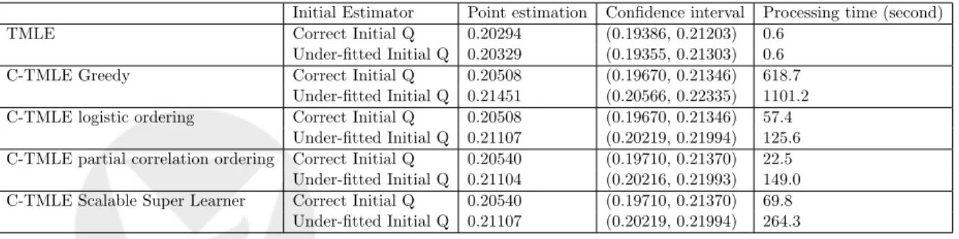
7.3.1 NOAC Study

Figure 4: Point estimate and 95% confidence interval for di↵erent C-TMLEs on NOAC data Fig. 4 shows the point estimate and 95% confidence interval for di↵erent C-TMLEs on NOAC data. We see that the point estimates from all C-TMLEs shift down when hdPS covariates are included. The estimated variances for C-TMLEs improved with the help of hdPS covariates. It is interesting that the confidence interval of logistic ordering shrinked significantly after adding hdPS covariates. In addition, logistic ordering with hdPS covariates resulted in a similar point estimate as TMLE, but with much smaller confidence interval. Both SL-CTMLEs produced a statistically significant result with and without the inclusion of hdPS covariates. In this analysis SL-CTMLE selected the partial correlation C-TMLE.

(19)

7.3.2 NSAID Study

Figure 5: Point estimate and 95% confidence interval for di↵erent C-TMLE on NSAID data Figute 5 shows the point estimate and 95% confidence interval for di↵erent C-TMLEs on NSAID data. After adding hdPS covariates, the point estimates shifted slightly to the right, with very little change in the CI width. This suggests the inclusion of hdPS covariates did little to reduce bias or variance in the parameter estimate.

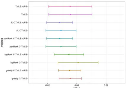
7.3.3 Vytorin Study

Figure 6: Point estimate and 95% confidence interval for di↵erent C-TMLE on VYTORIN data Fig. 6 shows the point estimate and 95% confidence interval for di↵erent C-TMLEs on Vytorin data. For this study, including hdPS covariates made no significant di↵erence. In addition, all

(20)

confidence intervals cover the null, with similar width. SL-CTMLE selected the logistic C-TMLE when hdPS covariates were not available. The partial correlation C-TMLE, logistic C-TMLE and SL-CTMLE had identical performance when hdPS covariates were made available.

7.4 Remarks

The NOAC study illustrates that including hdPS covariates can sometimes shift the point estimate and narrow confidence intervals. This suggests hdPS covariates can help reduce bias in the param-eter estimate. In addition, the confidence intervals for all C-TMLEs was smaller after adding hdPS covariates, which suggests hdPS can reduce the variance of the estimation. However, in the NSAID and Vytorin study, including hdPS covariates did not make a significant di↵erence for both point estimation and confidence intervals.

Including hdPS covariates dramatically increases the dimensionality of the data. The targeting step of the standard TMLE relies on propensity scores that are estimated without regard to the outcome. These models may have ignored information on confounders that are only weakly pre-dictive of treatment. In contrast, C-TMLE builds a propensity score model in response to residual bias. The greedy C-TMLE is not scalable with respect to the number of covariates, which leads to unacceptable long processing time. In this case, we suggest combining baseline and hdPS co-variates and using a pre-ordered C-TMLE to estimate the target parameter. Though the point estimates and confidence intervals for di↵erent C-TMLEs are often similar, in some cases they may vary substantially (for example in NOAC study). For more reliable estimation we encourage using SL-CTMLE to select the optimal scalable C-TMLE.

8 Time Complexity

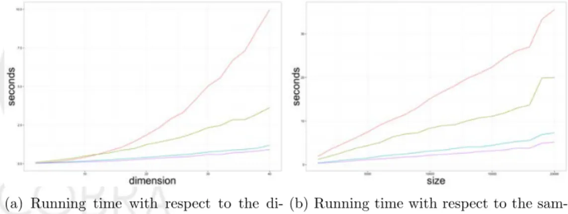
In this section, we study the computational efficiency of the preordering C-TMLEs. The processing time of the algorithm depends on the sample size n and the number of covariates p. To compare the running time for C-TMLE with di↵erent search strategies, we first fix the sample sizen= 1000, then variedIn theory p between 2 and 40 (Fig. 7, left). We then fixed the number of covariates to

p = 20, and varied n from 1000 to 20000 (Fig. 7, right). To make the processing time stable, for each pair of sample size and dimension, we repeated the analysis ten times and report the median processing time.

(a) Running time with respect to the di-mension (p) with fixed sample size (n)

(b) Running time with respect to the sam-ple size (n) with fixed dimension(p)

Figure 7: Running time for C-TMLE with greedy search and preordering. Red: greed forward selection C-TMLE; Green: SL-CTMLE with logistic ordering and partial correlation ordering in the library; Blue: C-TMLE with logistic ordering; Purple: C-TMLE with partial correlation ordering.

(21)

Fig. 7a shows the running time with respect to the dimension (p) with fixed observation size (n). In theory, the time complexity for forward stepwise and Super Learner C-TMLE is _O(p2_), while for pre-ordered C-TMLEs are O(p). The simulation results match the theory. For data sets with 1000 samples and 40 covariates, pre-ordered C-TMLE only took about 2 seconds. We can see the pre-ordered methods are scalable with high dimensional data.

Fig. 7b shows the running time with respect to the sample size (n) with fixed dimension(p). Theoretical, all the methods have time complexity_O(n). However, the pre-ordered C-TMLEs are much faster in practice.

9 C-TMLE package

Flexible software that implements all C-TMLEs described in this paper is publicly available at

https://lendle.github.io/TargetedLearning.jl/. The package contains options for

decreas-ing computation time of the scalable TMLEs.

The Pre-Ordered search strategy in the package has a second optional argument, k, which defaults to 1. At each step, the next k (or all available, if the remaining covariates is fewer than

k) ordered covariates are added to the next estimate of g0. Large k can speed up the procedure when there are many covariates. However, this approach is prone to overfitting, and may miss the optimal solution.

An early stopping criteria that avoids computing and cross-validating for the complete model can also save unnecessary computation. To accelerate the training, there is a patience option in the package. This argument fixes the number of steps to continue after finding a local optimum. For example, if we set patience to be 10, as in the Simulation Study presented in Section 6.4.1, then the program will automatically halt if the penalized cross-validated risk does not decrease for the next 10 covariates. The estimator with the best penalized CV-risk among the constructed candidates will be selected.

In addition to the two preordering methods described above, the software accepts any user-defined ranking algorithm.

10 Discussion

Double robust estimations like A-IPTW and traditional TMLE rely on the external estimation of the nuisance parameters. This practice is guided by the accuracy of the estimation of nuisance parameters rather than the parameter of interest. Instead, the C-TMLE algorithm estimates the nuisance parameters with consideration for the bias-variance trade-o↵ towards the parameter of interest. It uses a targeted penalized loss function to make smart choices in determining what variables to adjust for in the estimate of the propensity score and only adjusts for variables which have not been fully adjusted for in the initial estimate of the outcome.

To build a nested sequence of nuisance parameters models, a greedy forward stepwise selection algorithm originally proposed for C-TMLE implementation. However, the greedy search has rela-tively high time complexity, which makes it infeasible in analyses of large scale and high dimensional data. In this article, we proposed two pre-ordering procedures for C-TMLE that reduces the time complexity with respect to dimension p to the linear order. As the performance of pre-ordered C-TMLE relies on the predefined covariate order, a scalable SL-CTMLE framework is proposed to select the candidate C-TMLE with the best cross-validated fit.

Simulation studies demonstrated the performance and time efficiency of the scalable collab-orative targeted maximum likelihood estimation. The results showed that the greedy C-TMLE,

(22)

pre-ordered C-TMLEs and SL-CTMLE perform at least as well as the best performing estimators under every simulation scenario and that these C-TMLE based estimators had similar performance to each other. This suggests that the logistic ordering and partial correlation ordering are two pre-ordering strategies that can be used to reduce the computational burden of C-TMLE. Though these two ordering worked well in the simulations, SL-CTMLE framework o↵ers additional robust-ness, in the case of that one ordering fails. Though this study focus on the binary treatment, our framework can be adapted to a multi-level or continuous treatment by employing a working marginal structure model. We leave these extension as future work. In conclusion, the proposed pre-ordering C-TMLE provides a scalable implementation of collaborative targeted maximum like-lihood estimation for large scale and high-dimensional data.

References

[1] M Alan Brookhart, Sebastian Schneeweiss, Kenneth J Rothman, Robert J Glynn, Jerry Avorn, and Til St¨urmer. Variable selection for propensity score models. American Journal of Epi-demiology, 163(12):1149–1156, 2006.

[2] Jessica M Franklin, Sebastian Schneeweiss, Jennifer M Polinski, and Jeremy A Rassen. Plas-mode simulation for the evaluation of pharmacoepidemiologic methods in complex healthcare databases. Computational Statistics & Data Analysis, 72:219–226, 2014.

[3] David A Freedman and Richard A Berk. Weighting regressions by propensity scores.Evaluation Review, 32(4):392–409, 2008.

[4] Gary L Gadbury, Qinfang Xiang, Lin Yang, Stephen Barnes, Grier P Page, and David B Allison. Evaluating statistical methods using plasmode data sets in the age of massive public databases: an illustration using false discovery rates. PLoS Genet, 4(6):e1000098, 2008. [5] S. Gruber and M.J. van der Laan. A targeted maximum likelihood estimator of a causal e↵ect

on a bounded continuous outcome. The International Journal of Biostatistics, 6(1), 2010. [6] Susan Gruber and Mark J van der Laan. An application of collaborative targeted maximum

likelihood estimation in causal inference and genomics.The International Journal of Biostatis-tics, 6(1), 2010.

[7] Joseph F Hair, William C Black, Barry J Babin, Rolph E Anderson, and Ronald L Tatham. Multivariate Data Analysis, volume 6. Pearson Prentice Hall Upper Saddle River, NJ, 2006. [8] M. A. Hernan, B. Brumback, and J. M. Robins. Marginal structural models to estimate the

causal e↵ect of zidovudine on the survival of HIV-positive men. Epidemiology, 11(5):561–570, 2000.

[9] Cheng Ju, Mary Combs, Samuel D. Lendle, Jessica M. Franklin, Richard Wyss, Sebastian Schneeweiss, and Mark J van der Laan. Propensity score prediction for electronic healthcare dataset using super learner and high-dimensional propensity score method. 2016.

[10] Maya L Petersen, Kristin E Porter, Susan Gruber, Yue Wang, and Mark J van der Laan. Diagnosing and responding to violations in the positivity assumption. Statistical Methods in Medical Research, page 0962280210386207, 2010.

(23)

[11] J. M. Robins and A. Rotnitzky. Comment on the Bickel and Kwon article, ‘Inference for semiparametric models: Some questions and an answer’. Statistica Sinica, 11(4):920–936, 2001.

[12] J. M. Robins, A. Rotnitzky, and M.J. van der Laan. Comment on “On Profile Likelihood” by S.A. Murphy and A.W. van der Vaart. Journal of the American Statistical Association – Theory and Methods, 450:431–435, 2000.

[13] J.M. Robins. A new approach to causal inference in mortality studies with sustained exposure periods - application to control of the healthy worker survivor e↵ect. Mathematical Modelling, 7:1393–1512, 1986.

[14] J.M. Robins. Marginal structural models versus structural nested models as tools for causal inference. In Statistical Models in Epidemiology, the Environment, and Clinical Trials (Min-neapolis, MN, 1997), pages 95–133. Springer-Verlag, New York, 2000.

[15] J.M. Robins. Robust estimation in sequentially ignorable missing data and causal inference models. InProceedings of the American Statistical Association: Section on Bayesian Statistical Science, pages 6–10, 2000.

[16] Sebastian Schneeweiss, Jeremy A Rassen, Robert J Glynn, Jerry Avorn, Helen Mogun, and M Alan Brookhart. High-dimensional propensity score adjustment in studies of treatment e↵ects using health care claims data. Epidemiology (Cambridge, Mass.), 20(4):512, 2009. [17] Ori M Stitelman and Mark J van der Laan. Collaborative targeted maximum likelihood for

time to event data. The International Journal of Biostatistics, 6(1), 2010.

[18] Ori M Stitelman, C William Wester, Victor De Gruttola, and Mark J van der Laan. Targeted maximum likelihood estimation of e↵ect modification parameters in survival analysis. The International Journal of Biostatistics, 7(1):1–34, 2011.

[19] Aad W Vaart, Sandrine Dudoit, and Mark J Laan. Oracle inequalities for multi-fold cross validation. Statistics & Decisions, 24(3):351–371, 2006.

[20] Mark J Van Der Laan and Sandrine Dudoit. Unified cross-validation methodology for selection among estimators and a general cross-validated adaptive epsilon-net estimator: Finite sample oracle inequalities and examples. 2003.

[21] Mark J van der Laan and Susan Gruber. Collaborative double robust targeted maximum likelihood estimation. The International Journal of Biostatistics, 6(1), 2010.

[22] Mark J van der Laan, Eric C Polley, and Alan E Hubbard. Super learner. Statistical Applica-tions in Genetics and Molecular Biology, 6(1), 2007.

[23] Mark J Van der Laan and Sherri Rose. Targeted Learning: Causal Inference for Observational and Experimental Data. Springer Science & Business Media, 2011.

[24] Mark J van der Laan and Daniel Rubin. Targeted maximum likelihood learning. The Inter-national Journal of Biostatistics, 2(1), 2006.

[25] Hui Wang, Sherri Rose, and Mark J van der Laan. Finding quantitative trait loci genes with collaborative targeted maximum likelihood learning. Statistics & Probability Letters, 81(7):792–796, 2011.