Accelerating ADMM for efficient simulation and optimization

(1)

JUYONG ZHANG

∗†

_,

_{University of Science and Technology of China}

YUE PENG

∗

_,

WENQING OUYANG

∗

_,

BAILIN DENG,

Cardiff University

Target Mesh Initial Mesh Optimized Mesh

ADMM Ours

0 0.005

Planarity Error

Normalized Combined Residual

#V: 2570 #F: 2475

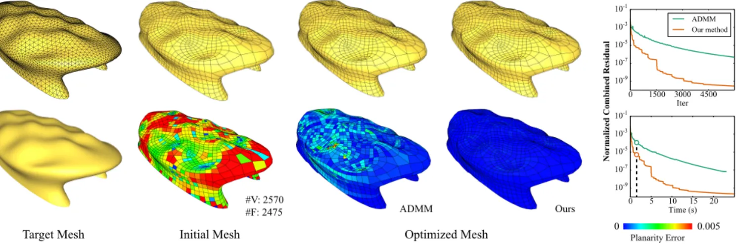
Fig. 1. We apply our accelerated ADMM solver to optimize a quad mesh, subject to hard constraints of face planarity and soft constraints of closeness to a reference surface. Our solver leads to a faster decrease of combined residual than the original ADMM, achieving better satisfaction of hard constraints within the same computational time (highlighted in the plot in bottom right).

The alternating direction method of multipliers (ADMM) is a popular ap-proach for solving optimization problems that are potentially non-smooth and with hard constraints. It has been applied to various computer graph-ics applications, including physical simulation, geometry processing, and image processing. However, ADMM can take a long time to converge to a solution of high accuracy. Moreover, many computer graphics tasks involve non-convex optimization, and there is often no convergence guarantee for ADMM on such problems since it was originally designed for convex op-timization. In this paper, we propose a method to speed up ADMM using Anderson acceleration, an established technique for accelerating fixed-point iterations. We show that in the general case, ADMM is a fixed-point iteration of the second primal variable and the dual variable, and Anderson accelera-tion can be directly applied. Addiaccelera-tionally, when the problem has a separable target function and satisfies certain conditions, ADMM becomes a fixed-point iteration of only one variable, which further reduces the computational overhead of Anderson acceleration. Moreover, we analyze a particular non-convex problem structure that is common in computer graphics, and prove the convergence of ADMM on such problems under mild assumptions. We

∗_{Equal contributions.} †

Corresponding author ([email protected]).

Authors’ addresses:{Juyong Zhang, Yue Peng, Wenqing Ouyang}, University of Science and Technology of China, 96 Jinzhai Road, Hefei 230026, Anhui, China, {[email protected], [email protected], [email protected]}; Bailin Deng, Cardiff University, 5 The Parade, Cardiff CF24 3AA, Wales, United Kingdom, [email protected].

This is the author’s version of the work. It is posted here for your personal use. Not for redistribution. The definitive Version of Record was published in_{ACM Transactions on} Graphics, https://doi.org/10.1145/3355089.3356491.

apply our acceleration technique on a variety of optimization problems in computer graphics, with notable improvement on their convergence speed.

CCS Concepts: •Computing methodologies→Computer graphics;

Animation; •Theory of computation→_{Nonconvex optimization}; Additional Key Words and Phrases: Physics Simulation, Geometry Optimiza-tion, ADMM, Anderson Acceleration

ACM Reference Format:

Juyong Zhang, Yue Peng, Wenqing Ouyang, and Bailin Deng. 2019. Acceler-ating ADMM for Efficient Simulation and Optimization.ACM Trans. Graph. 38, 6, Article 163 (November 2019), 21 pages. https://doi.org/10.1145/3355089. 3356491

1 INTRODUCTION

Many tasks in computer graphics involve solving optimization

prob-lems. For example, a geometry processing task may compute the

vertex positions of a deformed mesh by minimizing its deformation

energy [Sorkine and Alexa 2007], whereas a physical simulation

task may optimize the node positions of a system to enforce physics

laws that govern its behavior [Martin et al. 2011; Schumacher et al.

2012]. Such tasks are often formulated asunconstrained optimiza-tion, where the target function penalizes the violation of certain

conditions so that they are satisfied as much as possible by the

solu-tion. It has been an active research topic to develop fast numerical

solvers for such problems, with various methods proposed in the

past [Sorkine and Alexa 2007; Liu et al. 2008; Bouaziz et al. 2012;

Liu et al. 2013; Bouaziz et al. 2014; Wang 2015; Kovalsky et al. 2016;

(2)

On the other hand, some applications involve optimization with

hard constraints, i.e., conditions that need to be enforced strictly. Suchconstrainedoptimization problems are often more difficult to solve [Nocedal and Wright 2006]. One possible solution strategy is

to introduce a quadratic penalty term for the hard constraints with

a large weight, thereby converting it into an unconstrained

prob-lem that is easier to handle. However, to strictly enforce the hard

constraints, their penalty weight needs to approach infinity

[No-cedal and Wright 2006], which can cause instability for numerical

solvers. More sophisticated techniques, such as sequential quadratic

programming or the interior-point method, can enforce constraints

without stability issues. However, these solvers often incur high

com-putational costs and may not meet the performance requirements

for graphics applications. It becomes even more challenging for

non-smooth problems where the target function is not everywhere

differentiable, as many constrained optimization solvers require

gradient information and may not be applicable for such cases.

In recent years, the alternating direction method of multipliers

(ADMM) [Boyd et al. 2011] has become a popular approach for

solv-ing optimization problems that are potentially non-smooth and with

hard constraints. The key idea is to introduce auxiliary variables

and derive an equivalent problem with a separable target function,

subject to a linear compatibility constraint between the original

variables and the auxiliary variables [Combettes and Pesquet 2011].

ADMM searches for a solution to this converted problem by

al-ternately updating the original variables, the auxiliary variables,

and the dual variables. With properly chosen auxiliary variables,

each update step can reduce to simple sub-problems that can be

solved efficiently, often in parallel with closed-form solutions. In

addition, ADMM does not rely on the smoothness of the problem,

and converges quickly to a solution of moderate accuracy [Boyd

et al. 2011]. Such properties make ADMM an attractive choice for

solving large-scale optimization problems in various applications

such as signal processing [Chartrand and Wohlberg 2013; Simonetto

and Leus 2014], image processing [Figueiredo and Bioucas-Dias

2010; Almeida and Figueiredo 2013], and computer vision [Liu et al.

2013]. Recently, ADMM has also been applied for computer graphics

problems such as geometry processing [Bouaziz et al. 2013;

Neu-mann et al. 2013; Zhang et al. 2014; Xiong et al. 2014; NeuNeu-mann et al.

2014], physics simulation [Gregson et al. 2014; Pan and Manocha

2017; Overby et al. 2017], and computational photography [Heide

et al. 2016; Xiong et al. 2017; Wang et al. 2018].

Despite the effectiveness and versatility of ADMM, there are

still two major limitations for its use in computer graphics. First,

although ADMM converges quickly in initial iterations, its final

con-vergence might be slow [Boyd et al. 2011]. This makes it impractical

for problems with a strong demand for solution accuracy, such as

those with strict requirements on the satisfaction of hard constraints.

Recent attempts to accelerate ADMM such as [Goldstein et al. 2014;

Kadkhodaie et al. 2015; Zhang and White 2018] are only designed

for convex problems, which limits their applications in computer

graphics. Second, ADMM was originally designed for convex

prob-lems, whereas many computer graphics tasks involve non-convex

optimization. Although ADMM turns out to be effective for many

convex problems in practice, its convergence for general

non-convex optimization remains an open research question. Recent

convergence results such as [Li and Pong 2015; Hong et al. 2016;

Magnússon et al. 2016; Wang et al. 2019] rely on strong assumptions

that are not satisfied by many computer graphics problems.

This paper addresses these two issues of ADMM. First, we propose

a method to accelerate ADMM for non-convex optimization

prob-lems. Our approach is based on Anderson acceleration [Anderson

1965; Walker and Ni 2011], a well-established technique for

acceler-ating fixed-point iterations. Previously, Anderson acceleration has

been applied to local-global solvers for unconstrained optimization

problems in computer graphics [Peng et al. 2018]. Our approach

expands its applicability to many constrained optimization

prob-lems as well as other unconstrained probprob-lems where local-solver

solvers are not feasible. To this end, we need to solve two

prob-lems: (i) we must find a way to interpret ADMM as a fixed-point

iteration; (ii) as Anderson acceleration can become unstable, we

should define criteria to accept the accelerated iterate and a fall-back

strategy when it is not accepted, similar to [Peng et al. 2018]. We

show that in the general case ADMM is a fixed-point iteration of the

second primal variable and the dual variable, and we can evaluate

the effectiveness of an accelerated iterate via itscombined residual which is known to vanish when the solver converges. Moreover,

when the problem structure satisfies some mild conditions, one of

these two variables can be determined from the other one; in this

case ADMM becomes a fixed-point iteration of only one variable

with less computational overhead, and we can accept an accelerated

iterate based on a more simple condition. We apply this method to

a variety of ADMM solvers for computer graphics problems, and

observe a notable improvement in their convergence rates.

Additionally, we provide a new convergence proof of ADMM on

non-convex problems, under weaker assumptions than the

conver-gence results in [Li and Pong 2015; Hong et al. 2016; Magnússon et al.

2016; Wang et al. 2019]. For a particular problem structure that is

common in computer graphics, we also provide sufficient conditions

for the global linear convergence of ADMM. Our proofs shed new

light on the convergence properties of non-convex ADMM solvers.

2 RELATED WORK

Optimization solvers in computer graphics.The development of efficient optimization solvers has been an active research topic in

computer graphics. One particular type of method, called

local-global solvers, has been widely used for unconstrained optimization

in geometry processing and physical simulation. For geometry

pro-cessing, Sorkine and Alexa [2007] proposed a local-global approach

to minimize deformation energy for as-rigid-as-possible mesh

sur-face modeling. Liu et al. [2008] developed a similar method to

per-form conper-formal and isometric parameterization for triangle meshes.

Bouaziz et al. [2012] extended the approach to a unified

frame-work for optimizing discrete shapes. For physical simulation, Liu

et al. [2013] proposed a local-global solver for optimization-based

simulation of mass-spring systems. Bouaziz et al. [2014] extended

this approach to the projective dynamics framework for implicit

time integration of physical systems via energy minimization.

Local-global solvers often converge quickly to an approximate

solution, but may be slow for final convergence. Other methods

(3)

geometry processing, Kovalsky et al. [2016] achieved a fast

con-vergence of geometric optimization by iteratively minimizing a

local quadratic proxy function. Rabinovich et.al. [2017] proposed

a scalable approach to compute locally injective mappings, via

local-global minimization of a reweighted proxy function. Claici et

al. [2017] proposed a preconditioner for fast minimization of

distor-tion energies. Shtengel et al. [2017] applied the idea of majorizadistor-tion-

majorization-minimization [Lange 2004] to iteratively update and minimize a

convex majorizer of the target energy in geometric optimization.

Zhu et al. [2018] proposed a fast solver for distortion energy

min-imization, using a blended quadratic energy proxy together with

improved line-search strategy and termination criteria. For

physi-cal simulation, Wang [2015] proposed a Chebyshev semi-iterative

acceleration technique for projective dynamics. Later, Wang and

Yang [2016] developed a GP U-friendly gradient descent method for

elastic body simulation, using Jacobi preconditioning and

Cheby-shev acceleration. Liu et al. [2017] proposed an L-BFGS solver for

physical simulation, with faster convergence than the projective

dynamics solver from [Bouaziz et al. 2014]. Brandt et al. [2018]

per-formed projective dynamics simulation in a reduced subspace, to

compute fast approximate solutions for high-resolution meshes.

ADMM. ADMM is a popular solver for optimization problems with separable target functions and linear side constraints [Boyd

et al. 2011]. Using auxiliary variables and indicator functions, such

formulation allows for non-smooth optimization with hard

con-straints, with wide applications in signal processing [Erseghe et al.

2011; Simonetto and Leus 2014; Shi et al. 2014], image

process-ing [Figueiredo and Bioucas-Dias 2010; Almeida and Figueiredo

2013], computer vision [Hu et al. 2013; Liu et al. 2013; Yang et al.

2017], computational imaging [Chan et al. 2017], automatic

con-trol [Lin et al. 2013], and machine learning [Zhang and Kwok 2014;

Hajinezhad et al. 2016]. ADMM has also been used in computer

graphics to handle non-smooth optimization problems [Bouaziz

et al. 2013; Neumann et al. 2013; Zhang et al. 2014; Xiong et al.

2014; Neumann et al. 2014] or to benefit from its fast initial

conver-gence [Gregson et al. 2014; Heide et al. 2016; Xiong et al. 2017; Pan

and Manocha 2017; Overby et al. 2017; Wang et al. 2018].

ADMM was originally designed for convex optimization [Gabay

and Mercier 1976; Fortin and Glowinski 1983; Eckstein and Bertsekas

1992]. For such problems, its global linear convergence has been

established in [Lin et al. 2015; Deng and Yin 2016; Giselsson and Boyd

2017], but these proofs require both terms in the target function to be

convex. In comparison, our proof of global linear convergence allows

for non-convex terms in the target function, which is better aligned

with computer graphics problems. In practice, ADMM works well for

many non-convex problems as well [Wen et al. 2012; Chartrand 2012;

Chartrand and Wohlberg 2013; Miksik et al. 2014; Lai and Osher

2014; Liavas and Sidiropoulos 2015], but it is more challenging to

establish its convergence for general non-convex problems. Only

very recently have such convergence proofs been given under strong

assumptions [Li and Pong 2015; Hong et al. 2016; Magnússon et al.

2016; Wang et al. 2019]. We provide in this paper a general proof of

convergence for non-convex problems under weaker assumptions.

It is well known that ADMM converges quickly to an approximate

solution, but may take a long time to convergence to a solution of

high accuracy [Boyd et al. 2011]. This has motivated researchers to

explore acceleration techniques for ADMM. Goldstein et al. [2014]

and Kadkhodaie et al. [2015] applied Nesterov’s acceleration

[Nes-terov 1983], whereas Zhang and White [2018] applied GMRES

ac-celeration to a special class of problems where the ADMM iterates

become linear. All these methods are designed for convex problems

only, which limits their applicability in computer graphics.

Anderson acceleration. Anderson acceleration [Walker and Ni 2011] is an established technique to speed up the convergence of

a fixed-point iteration. It was first proposed in [Anderson 1965]

for solving nonlinear integral equations, and independently

re-discovered later by Pulay [1980; 1982] for accelerating the

self-consistent field method in quantum chemistry. Its key idea is to

utilize themprevious iterates to compute a new iterate that con-verges faster to the fixed point. It is indeed a quasi-Newton method

for finding a root of the residual function, by approximating its

inverse Jacobian using previous iterates [Eyert 1996; Fang and Saad

2009; Rohwedder and Schneider 2011]. Recently, a renewed interest

in this method has led to the analysis of its convergence [Toth and

Kelley 2015; Toth et al. 2017], as well as its application in various

numerical problems [Sterck 2012; Lipnikov et al. 2013; Pratapa et al.

2016; Suryanarayana et al. 2019; Ho et al. 2017]. Peng et al. [Peng

et al. 2018] noted that local-global solvers in computer graphics

can be treated as fixed-point iteration, and applied Anderson

ac-celeration to improve their convergence. Additionally, to address

the stability issue of classical Anderson acceleration [Walker and

Ni 2011; Potra and Engler 2013], they utilize the monotonic energy

decrease of local-global solvers and only accept an accelerated

it-erate when it decreases the target energy. Fang and Saad [2009]

called classical Anderson acceleration the Type-II method in an

Anderson family of multi-secant methods. Another member of the

family, called the type-I method, uses quasi-Newton to approximate

the Jacobian of the fixed-point residual function instead [Walker

and Ni 2011], and has been analyzed recently in [Zhang et al. 2018].

In this paper, we focus our discussion on the type-II method.

3 OUR METHOD 3.1 Preliminary

ADMM.Let us consider an optimization problem min

x Φ(x,Dx+h). (1)

Herexcan be the vertex positions of a discrete geometric shape, or the node positions of a physical system at a particular time instance.

The quantityDx+hencodes a transformation of the positionsx relevant for the optimization problem, such as the deformation

gra-dient of each tetrahedron element in an elastic object. The notation Φ(x,Dx+h)signifies that the target function contains a term that directly depends onDx+h, such as elastic energy dependent on the deformation gradient. In some applications, the optimization

enforceshard constraintsonxorDx+h, i.e., conditions that need to be strictly satisfied by the solution. Such hard constraints can be

encoded using anindicator functionterm within the target function. Specifically, suppose we want to enforce a conditiony∈ Cwherey is a subset from the components ofxorDx+h, andCis thefeasible

(4)

set. Then we include the following term intoΦ: σC(y)=

0 ify∈ C

+∞ otherwise .

By definition, ifx∗is a solution, then the corresponding components y∗must satisfyy∗∈ C; otherwise it will result in a target function value+∞instead of the minimum. Examples of such an approach to modeling hard constraints can be found in [Deng et al. 2015].

In many applications, the optimization problem (1) can be

non-linear, non-convex, and potentially non-smooth. It is challenging to

solve such a problem numerically, especially when hard constraints

are involved. One common technique is to introduce an auxiliary

variablez=Dx+hto derive an equivalent problem min

x,z Φ(x,z)

s.t.W(z−Dx−h)=0, (2)

whereWis a diagonal matrix with positive diagonal elements.W can be the identity matrix in the trivial case, or a diagonal

scal-ing matrix that improves conditionscal-ing [Giselsson and Boyd 2017;

Overby et al. 2017]. ADMM [Boyd et al. 2011] is widely used to solve

such problems. For ease of discussion, let us consider the problem

min

x,z Φ(x,z) s.t.Ax−Bz=c, (3)

Its solution corresponds to a stationary point of the augmented

Lagrangian function L(x,z,u)=Φ(x,z)+⟨µu,Ax−Bz−c⟩+µ 2 ∥Ax−Bz−c∥2 =Φ(x,z)+µ 2 ∥Ax−Bz+u−c∥2 −µ 2 ∥u∥2 . (4)

Hereuis thedual variableandµ > 0 is the penalty parameter. Following [Boyd et al. 2011], we also callxandztheprimal variables. ADMM searches for a stationary point by alternately updatingx,z andu, resulting in the following iteration scheme [Boyd et al. 2011]:

xk+1 =argmin x L (x,zk,uk), zk+1= argmin z L(xk+1, z,uk), uk+1 =uk+Axk+1 −Bzk+1 −c. (5)

We can also updatezbeforex, resulting in an alternative scheme:

zk+1 =argmin z L (xk,z,uk), xk+1 =argmin x L(x,zk+1 ,uk), uk+1 =uk+Axk+1 −Bzk+1 −c. (6)

In this paper, we refer to the scheme (5) asx-z-uiteration, and the scheme (6) asz-x-uiteration. In both cases, the updates forzandx often reduce to simple subproblems that can potentially be solved

in parallel. According to [Boyd et al. 2011], the optimality condition

of ADMM is that both itsprimal residualanddual residualvanish. For both iteration schemes above, the primal residual is defined as

rk+1

p =Axk+ 1

−Bzk+1

−c.

As for the dual residual: for thex-z-uiteration it is defined as

rk+1

d =µA

T_B₍_zk+1

−zk), (7)

whereas for thez-x-uiteration it is defined as

rk+1

d =µB

T_A₍_xk+1

−xk). (8)

Intuitively, the primal residual measures the violation of the linear

side constraint, whereas the dual residual measures the violation of

the dual feasibility condition [Boyd et al. 2011]. Accordingly, ADMM

is terminated when both∥rk+1

p ∥and∥rk+ 1 d ∥

are small enough.

Anderson acceleration.ADMM is easy to parallelize and conver-gences quickly to an approximate solution. However, it can take a

long time to converge to a solution of high accuracy [Boyd et al.

2011]. In the following subsections, we will discuss how to apply

Anderson acceleration [Walker and Ni 2011] to improve its

gence. Anderson acceleration is a technique to speed up the

conver-gence of a fixed-point iterationG:_Rn7→_Rn, by utilizing the cur-rent iterate as well asmprevious iterates. Letqk−m,qk−m+1, . . . ,qk be the latestm+1 iterates, and denote their residuals under map-pingG asFk−m,Fk−m+1, . . . ,Fk, whereFj = G(qj) −qj (j = k−m, . . . ,k). Then the accelerated iterate is computed as

qk+1 AA = (1−β) © « qk− m Õ j=1 θ∗ j(qk−j+1−qk−j)ª ® ¬ +β© « G(qk) − m Õ j=1 θ∗ j(G(qk−j+1) −G(qk−j))ª ® ¬ , (9) where(θ∗ 1, . . . ,θ ∗

m)is the solution to a linear least-squares problem:

min (θ1, ...,θm) Fk− m Õ j=1 θj(Fk−j+1 −Fk−j) 2 . (10)

In Eq. (9),β ∈ (0,1] is a mixing parameter, and is typically set to 1 [Walker and Ni 2011]. We follow this convention throughout

this paper. Previously, Anderson acceleration has been applied to

speed up local-global solvers in computer graphics [Peng et al. 2018].

3.2 Anderson acceleration of ADMM: the general approach

To speed up ADMM with Anderson acceleration, we must first define

its iteration scheme as a fixed-point iteration. For thex-z-uiteration, we note thatxk+1is dependent only onzkanduk. Therefore, by treatingxk+1as a function of(zk,uk), we can rewritezk+1, and subsequentlyuk+1, as a function of(zk,uk)as well. In this way, the x-z-uiteration can be treated as a fixed-point iteration of(z,u):

(zk+1,

uk+1

)=G(zk,uk).

Similarly, we can treat thez-x-uscheme as a fixed-point iteration of (x,u). In addition, to ensure stability for Anderson acceleration, we should define criteria to evaluate the effectiveness of an accelerated

iterate, as well as a fall-back strategy when the criteria are not met.

Goldstein et al. [2014] pointed out that if the problem is convex,

then itscombined residualis monotonically decreased by ADMM. For thex-z-uiteration, the combined residual is defined as

rk+1 x-_z-_u=µ∥Axk+ 1 −Bzk+1 −c∥2+µ ∥B(zk+1 −zk)∥2. (11)

Here the first term is a measure of the primal residual, whereas the

(5)

Algorithm 1:Anderson acceleration for ADMM withx-z-uiteration.

Data: x0

,z0,u0: initial values of variables; L: the augmented Lagrangian function;

m: the number of previous iterates used for acceleration; AA(G,F): Anderson accleration from a sequenceGof fixed-point mapping results of previous iterates, and a sequenceFof their corresponding fixed-point residuals;

Imax: the maximum number of iterations; ε: convergence threshold for combined residual. 1 xdefault=x0

; zdefault=z0; udefault=u0; 2 rprev= +∞; j=0; reset = TRUE; k=0; 3 whileTRUEdo

// Run one iteration of ADMM 4 x⋆=argmin

xL(x,zk,uk); 5 z⋆=argmin

zL(x⋆,z,uk); 6 u⋆=uk+Ax⋆−Bz⋆−c;

// Compute the combined residual 7 r=∥Ax⋆−Bz⋆−c∥2

+∥B(z⋆−zk) ∥2 ; 8 if reset == TRUEORr<rprevthen

// Record the latest accepted iterate

9 xdefault=x⋆; zdefault=z_⋆; udefault=u_⋆;

10 rprev=r;reset = FALSE;

// Compute the accelerated iterate 11 gj=(z⋆,u⋆); f_j =(z_⋆−zk,u_⋆−uk); 12 j=j+1; m=min(m−1,j); 13 (zk+1,uk+1)=AA [g_j, . . . ,g_j −m],[fj, . . . ,fj−m] ; 14 k=k+1; 15 else

// Revert to the last accepted iterate

16 zk=zdefault; uk=udefault; reset = TRUE;

17 end if

18 ifk ≥Imax ORr<εthen // Check termination

19 returnxdefault; // Return the last accepted x 20 end if

21 end while

AT. The combined residual for thez-x-uiteration is defined as rk+1 z-_x-_u=µ∥Axk+ 1 −Bzk+1 −c∥2+µ ∥A(xk+1 −xk)∥2. (12)

Although [Goldstein et al. 2014] only proved the monotonic decrease

of the combined residual for convex problems, our experiments

show that the combined residual is decreased by the majority of

iterates from the non-convex ADMM solvers considered in this

pa-per. Indeed, if ADMM converges to a solution, then both the primal

residualAxk+1−Bzk+1−cand the variable changeszk+1−zkand

xk+1₋

xkmust converge to zero, so the combined residual must converge to zero as well. Therefore, we evaluate the effectiveness

of an accelerated iterate by checking whether it decreases the

com-bined residual compared with the previous iteration, and revert to

the un-accelerated ADMM iterate if this is not the case.

Algorithm 1 summarizes our Anderson acceleration approach for

thex-z-uiteration. Note that the evaluation of combined residual

requires computing the change ofzin one un-accelerated ADMM

iteration. However, given an accelerated iterate(zAA,uAA), it is

of-ten difficult to find a pair(z_†,u_†)that leads to(z_AA,u_AA)after one

Algorithm 2:Anderson acceleration for ADMM withz-x-uiteration. 1 xdefault=x0

;udefault=u0;rprev= +∞;j=0; reset = TRUE;k=0;

2 whileTRUEdo 3 z⋆=argmin zL(xk,z,uk); 4 x⋆=argmin xL(x,z⋆,uk); 5 u⋆=uk+Ax⋆−Bz⋆−c; 6 r=∥Ax⋆−Bz⋆−c∥2 +∥A(x⋆−xk) ∥2 ; 7 if reset == TRUEORr<rprevthen

8 xdefault=x⋆; udefault=u_⋆; rprev=r; reset = FALSE;

9 j=j+1; m=min(m−1,j); 10 gj=(x⋆,u⋆); f_j=(x_⋆−xk,u_⋆−uk); 11 (xk+1 ,uk+1 )=AA [g_j, . . . ,g_j₋_m],[f_j, . . . ,f_j₋_m]; 12 k=k+1; 13 else

14 xk =xdefault; uk =udefault; reset = TRUE;

15 end if

16 ifk ≥Imax ORr<εthen

17 returnxdefault; 18 end if

19 end while

ADMM iteration (i.e.,(zAA,uAA)=G(z†,u†)). Therefore, we run one ADMM iteration on(z_AA,u_AA)instead, and use the resulting values(z⋆,u⋆)=G(zAA,uAA)to evaluate the combined residual. If

the accelerated iterate is accepted, then the computation of(z_⋆,u_⋆) can be reused in the next step of the algorithm and incurs no

over-head. We can derive an acceleration method for thex-z-uiteration in a similar way, by swappingxandzand adopting Eq. (8) for the computation of combined residual, as summarized in Algorithm 2.

Remark3.1. If the target functionΦcontains an indicator function for a hard constraint on the primal variable updated in the second

step of an ADMM iteration (i.e.,zin thex-z-uiteration, orxin thez -x-uiteration), then after each iteration this variable must satisfy the hard constraint. However, as Anderson acceleration computes the

accelerated iterate via an affine combination of previous iterates, the

acceleratedzAAorxAAmay violate the constraint unless its feasible

set is an affine space. In other words, the accelerated iterate may not

correspond to a valid ADMM iteration, and may cause issues if it is

used as a solution. Therefore, to apply Anderson acceleration, we

should ensure thatΦcontains no indicator function associated with the primal variable updated in the second step of the original ADMM

iteration. This does not limit the applicability of our method, because

it can always be achieved by introducing auxiliary variables and

choosing an appropriate iteration scheme. The simulation in Fig. 4 is

an example of changing the iteration scheme to allow acceleration.

3.3 ADMM with a separable target function

The general approach in Section 3.2 does not assume any special

structure of the target function. When the target function terms

forxandzare separable, it is possible to improve the efficiency of acceleration further. To this end, we consider the following problem

min

x,z f(x)+д(z),

s.t.Ax−Bz=c. (13)

(6)

Assumption 3.1. MatrixBis invertible.

Assumption 3.2. f(x)is a strongly convex quadratic function f(x)=1

2

(x−x˜)TG(x−x˜), (14)

wherex˜is a constant andGis a symmetric positive definite matrix. One example of such optimization is the implicit time integration

of elastic bodies in [Overby et al. 2017], where ˜xis the predicted values of node positionsxwithout internal forces,G = M/∆t2 whereMis the mass matrix and∆tis the integration time step, the auxiliary variablezstacks the deformation gradient of each element, andд(z)sums the elastic potential energy for all elements. For the problem (13), thex-z-uiteration of ADMM becomes

xk+1= (G+µATA)−1 (Gx˜+µAT(Bzk+c−uk)), (15) zk+1 =argmin z д(z)+µ 2 ∥Axk+1 −Bz−c+uk∥2 , (16) uk+1 =uk+Axk+1 −Bzk+1 −c. (17)

And thez-x-uiteration becomes

zk+1 =argmin z д(z)+µ 2 ∥Axk−Bz−c+uk∥2 , (18) xk+1 =(G+µATA)−1 (Gx˜+µAT(Bzk+1+c−uk)), (19) uk+1 =uk+Axk+1 −_Bzk+1 −_c. (20)

Similar to Remark 3.1, we assume that the target function contains

no indicator function for the primal variable updated in the second

step. The general acceleration algorithms in Section 3.2 treat ADMM

as a fixed-point iteration of(z,u)or(x,u). Next, we will show that if the problem satisfies certain conditions, then ADMM becomes a

fixed-point iteration of only one variable, allowing us to reduce the

overhead of Anderson acceleration and improve its effectiveness.

Remark3.2. Without assuming the convexity of functionд(·), there may be multiple solutions for the minimization problems in (16)

and (18). Throughout this paper, we assume the solver adopts a

deterministic algorithm for (16) and (18), so that given the same

values ofxanduit always returns the same value ofz.

3.3.1 x-z-uiteration. For thex-z-uiteration (15)-(17), under cer-tain conditionsuk+1can be represented as a function ofzk+1:

Proposition 3.1. If the optimization problem(13)satisfies

As-sumptions 3.1 and 3.2, and the functionд(z)is differentiable, then the

x-z-uiteration(15)-(17)satisfies

uk+1

=1_µB−T∇д(zk+1

). (21)

A proof is given in Appendix A. Proposition 3.1 shows thatuk+1 can be recovered fromzk+1. Therefore, we can treat thex-z-u iter-ation (15)-(17) as a fixed-point iteriter-ation ofzinstead of(z,u), and apply Anderson acceleration tozalone. From the acceleratedzAA,

we recover its corresponding dual variableu_AAvia Eq. (21). This approach brings two major benefits. First, the main computational

overhead for Anderson acceleration in each iteration is to update

the normal equation system for the problem (10), which involves

inner products of time complexityO(mn)wherenis the dimension

Algorithm 3:Anderson acceleration for ADMM withx-z-u itera-tion, on a problem (13) that satisfies Assumptions 3.1, 3.2 and with a differentiableд.

1 rprev= +∞; j=0; reset = TRUE; k=0; 2 whileTRUEdo

// Updatex with(15) _{and compute residual with} (22)

3 xk+1

=(G+µATA)−1

(G_x˜+µAT_(Bzk+_c₋_uk₎₎; 4 r=∥Axk+1−Bzk−c∥;

5 ifreset == FALSEANDr ≥rprevthen // Check residual

6 zk =zdefault; _{// Revert to un-accelerated} z

// Re-compute u andx with (17) and (15)

7 uk =uk−1+Axk−Bzk−c;

8 xk+1=(G+µATA)−1(Gx˜+µAT(Bzk+c−uk)); // Re-compute residual

9 r =∥Axk+1−Bzk−c∥; reset = TRUE; 10 end if

// Check termination criteria 11 ifk+1≥ImaxORr<εthen 12 returnxk+1

; 13 end if

// Compute un-accelerated z value with (16)

14 zdefault=argmin z д(z)+µ2∥Ax k+1 −Bz−c+uk∥2

// Compute acceleratedz value

15 j=j+1; m=min(m,j);

16 gj=zdefault; f_j=zdefault−zk;

17 zk+1

=AA [g_j, . . . ,g_j₋_m],[f_j, . . . ,f_j₋_m];

// Recover compatibleu value with(21)

18 uk+1= 1_µB−T∇д(zk+1); 19 k=k+1; rprev=r; 20 end while

of variables that undergo fixed-point iteration [Peng et al. 2018].

SinceBis invertible,uandzare of the same dimension; thus this new approach reduces the computational cost of inner products by

half. Another benefit is a more simple criterion for the effectiveness

of an accelerated iterate, based on the following property:

Proposition 3.2. Suppose the problem(13)satisfies Assumptions 3.1

and 3.2, and the functionд(z)is differentiable. Letzk+1=G xzu(zk) denote the fixed-point iteration ofzinduced by thex-z-uiteration(15) -(17). Thenzk+1is a fixed point of mappingG_xzu(·)if and only if

Axk+2

−Bzk+1

−c=0. (22)

A proof is given in Appendix B. Note that the left-hand side of (22)

has a similar form as the primal residual, but involves the value of xin the next iteration. Accordingly, we evaluate the effectiveness of an accelerated iteratez_AAand its corresponding dual variable uAAby first computing a new valuex⋆according to thex-update

step (15), then evaluating a residual ˆr_x-z-u = Ax⋆−BzAA −c.

We only acceptz_AAif it leads to a smaller norm of this residual compared to the previous iteration; otherwise, we revert to the last

un-accelerated iterate. Ifz_AAis accepted, thenx_⋆can be reused in the next step. The main benefit here is that we do not need to run an

(7)

additional ADMM iteration to verify the effectiveness ofzAA, which

incurs less computational overhead when the accelerated iterate is

rejected. This acceleration strategy is summarized in Algorithm 3.

Fig. 2 shows an example where acceleratingzalone leads to a faster decrease of combined residual than acceleratingz,utogether.

3.3.2 z-x-uiteration.Similar to the previous discussion, when the problem satisfies certain conditions, thez-x-uscheme is a fixed-point iteration of only one variable. In particular, we have:

Proposition 3.3. If the optimization problem(13)satisfies

As-sumptions 3.1 and 3.2, then thez-x-uiteration(18)-(20)satisfies

xk+1

=x˜−µG−1ATuk+1. (23)

A proof is given in Appendix C. This property implies thatxk+1 can be recovered fromuk+1; thus we can treat thez-x-uscheme (18)-(20) as a fixed-point iteration ofuinstead of(x,u). In theory, we can apply Anderson acceleration to the history ofuto obtain an accelerated iterateuAA, and recover the correspondingxAAfrom

Eq. (23). However, this would require solving a linear system with

matrixG, and can be computationally expensive. Instead, we note thatxk+1anduk+1are related to by an affine map, and this relation is satisfied by any previous pair ofxanduvalues. Then sinceu_AA is an affine combination of previousuvalues, we can apply the same affine combination coefficients to the corresponding previous xvalues to obtainxAA, which is guaranteed to satisfy Eq. (23) with

uAA. As the affine combination coefficients are computed fromu

only, this still reduces the computational cost compared to applying

Anderson acceleration to(x,u). Similar to thex-z-ucase, we can verify the convergence of thez-x-uiteration by comparingxin the current iteration with the value ofzin the next iteration:

Proposition 3.4. Suppose the problem(13)satisfies Assumptions 3.1

and 3.2. Letuk+1 =G

zxu(uk)denote the fixed-point iteration ofu induced by thex-z-uiteration(18)-(20). Thenuk+1is a fixed point of

mappingGzxu(·)if and only if

Axk+1

−Bzk+2

−c=0. (24)

Accordingly, we evaluate the effectiveness ofuAAandxAAby

computing from them az_⋆using Eq. (18), and evaluating the residual ˆ

rz-x-u=AxAA−Bz⋆−c. We acceptuAAif the norm of this residual

is smaller than the previous iteration, and revert to the last

un-accelerated iterate otherwise. IfuAAis accepted, thenz⋆is reused

in the next step. Algorithm 4 summarizes our approach.

Remark3.3. We have shown that ADMM can be reduced to a fixed-point iteration of the second primal variable or the dual variable

based on Assumptions 3.1 and 3.2, and (for thex-z-uiteration) the smoothness ofд. In fact, these assumptions can be further relaxed. We refer the reader to Appendix E for more details. Fig. 11 is an

example of using such relaxed conditions to reduce the fixed-point

iteration to one variable.

Algorithm 4:Anderson acceleration for ADMM withz-x-uiteration, on a problem (13) that satisfies Assumptions 3.1 and 3.2.

1 rprev= +∞; j=0; reset = TRUE; k=0; 2 whileTRUEdo

// Updatez with (18) _{and compute residual with} (24)

3 zk+1 =argmin z д(z)+µ2∥Ax k₋_Bz₋_c₊_uk_∥2 ; 4 r=∥Axk−Bzk+1 −c∥;

// Check whether the residual increases 5 ifreset == FALSEANDr ≥rprevthen

// Revert to un-accelerated x,u 6 xk =xdefault; uk =udefault; 7 zk+1=argmin z д(z)+µ2∥Ax k₋_Bz₋_c₊_uk_∥2 ; 8 r =∥Axk−Bzk+1−c∥; 9 reset = TRUE; 10 end if 11 ifk+1≥ImaxORr<εthen 12 returnxk; 13 end if

// Compute un-accelerated x and u

14 xdefault=(G+µATA)−1

(Gx˜+µAT(Bzk+1+c−uk));

15 udefault=uk+Axdefault−Bzk+1

−c;

// Use history ofu to compute affine coeffients

16 j=j+1; m=min(m,j); 17 gx_j=xdefault; gu j=udefault; fu j =udefault−uk; 18 (θ1∗, . . . ,θ ∗ m)= argmin (θ1, ...,θm) f u j −Ími=1θi(f u j−i+1−f u j−i) 2 ;

// Compute acceleratedx and uwith the coefficients

19 xk+1 =gx_j−Ím i=1θ ∗ i gx_j₋_i₊1−g x j−i ; 20 uk+1 =gu_j−Ím i=1θ ∗ i gu_j₋_i₊1−g u j−i ; 21 k=k+1; rprev=r; 22 end while 3.4 Convergence analysis

For Anderson acceleration to be applicable, an ADMM solver must

be convergent already. However, many ADMM solvers used in

computer graphics lack a convergence guarantee due to the

non-convexity of the problems they solve. Although ADMM works well

for many non-convex problems in practice, convergence proofs on

such problems rely on strong assumptions that are often not satisfied

by graphics problems [Li and Pong 2015; Hong et al. 2016;

Magnús-son et al. 2016; Wang et al. 2019]. In this subsection, we discuss the

convergence of ADMM on the problem (13) where the termдin the target function can be non-convex. We first provide a set of

condi-tions for linear convergence of ADMM on such problems, and then

give more general convergence proofs using weaker assumptions

than existing results in the literature. As the problem structure (13)

is common in computer graphics, our new results can potentially

expand the applicability of ADMM for graphics problems.

To ease the presentation, we first introduce some notation. To

account for the fact that the target function may be unbounded from

above due to an indicator function, we suppose all the functions are

(8)

Fwe define its effective domain and level set as: dom(F)_B{x|f(x)<+∞},

LαF B{x|f(x) ≤α}, givenα ∈_R.

A functionFislevel-boundedifL_αF is a bounded set for anyα∈_R. Given a setS, letI_SandB_S denote the interior and the bound-ary ofS, respectively. A functionF is continuous on_Rn if: (i) it is continuous withinI_dom₍_F₎in the conventional sense; and (ii) ∀xk →x∈ Bdom(F), we haveF(x_k) →F(x)= +∞. We say a func-tion isLipschitz differentiableif it is differentiable and its gradient is Lipschitz continuous. Unless specified otherwise,Idenotes the iden-tity matrix and the ideniden-tity map. The symbol conv(S)denotes the convex hull of a setS, and∂Fdenotes the set of all sub-differentials for a functionF(see [Rockafellar and Wets 2009, Definition 8.3(b)]). For matrixQ, we useρ(Q)to represent its spectral radius. We will discuss conditions for the ADMM iterates{(xk,zk,uk)}to converge to a stationary point(x∗,z∗,u∗)of the augmented Lagrangian for problem (13), which is defined by the conditions [Boyd et al. 2011]:

Ax∗−Bz∗=c, 0∈∂f(x∗)+ATu∗, 0∈∂д(z∗) −BTu∗. (25)

Linear convergence. Our discussion involves the following defini-tions related to the problem (13) and Assumpdefini-tions 3.1 and 3.2:

ˆ

д(z)_Bд(B−1

z), KBAG−1AT. (26)

We denote byρ(K)the spectral radius of matrixK. To prove linear convergence of ADMM for the problem (13) regardless of its initial

value, we need the following assumption:

Assumption 3.3. ∇дˆis Lipschitz differentiable on_Rnwith a

Lips-chitz constantL, i.e.∥∇дˆ(z1) − ∇дˆ(z2)∥ ≤L∥z1−z2∥∀z1,z1∈Rn.

Then we have:

Theorem 3.1. If Assumptions 3.1-3.3 are satisfied andρ(K)< 1

2L, then for a sufficiently largeµthex-z-uiteration(15)-(17)converges

to a stationary point defined in Eq.(25). Moreover, ∥Bzn+1 −Bzn∥ ≤γ1∥Bzn−Bzn −1 ∥, whereγ1= µ ρ(K) 1+µ ρ(K)+ L µ 1−L µ <1is a constant.

Theorem 3.2. If Assumptions 3.1-3.3 are satisfied,ρ(K)< 1 LandI− µKis invertible, then for a sufficiently largeµthez-x-uiteration(18) -(20)converges to a stationary point defined in Eq.(25). Moreover,

∥vk+1 −vk∥ ≤γ2∥vk−vk −1∥, wherevk=(I−µK)ukandγ2= µ ρ(K) 1+µ ρ_(K)+ L µ−L <1.

Proofs are provided in Appendix F. The theorems above rely on

Assumption 3.3 which requires the functionдto be globally Lipschitz differentiable. This may not be the case for some graphics problems.

For example, the StVK energy used for simulation of hyperelastic

materials is a quartic function of the deformation gradient, and is

locally Lipschitz differentiable but not globally so. For such problems,

we can still prove linear convergence with additional conditions

on its initial value and penalty parameter. In the following, we use

T(x,z)to denote the target function (13). We make the following relaxed assumption about ˆд:

Assumption 3.4. (1) дˆis level-bounded, andдˆ(z) ≥0∀z∈_Rn.

(2)дˆis continuous on_Rnand differentiable inI_dom₍_д_ˆ).

(3)дˆis Lipschitz differentiable on any compact convex set indom(дˆ). For linear convergence of thex-z-uiteration, we assume the following for the initial value(x0,z0,u0)and penalty parameterµ: Assumption 3.5. (1) z0 =B−1(Ax0−c),u0 = 1_µB−T∇д(z0).

z0

∈dom(д).

(2) µis large enough such thatc1≤1, where

c1= sup z∈L_Tд0₊1 1 2µ ∥B−T∇д(z)∥2 andT0=T₍ x0, z0₎

. Moreover, supposeconv(L

ˆ

д T0+c

1

) ⊂dom(дˆ)

and letLcbe a Lipschitz constant of∇дˆover this set. Theorem 3.3. Suppose Assumptions 3.1, 3.2, 3.4, 3.5 are satisfied, µ 2− L2 c µ >L2c, andρ(K)< 1

2L_c. Then for a sufficiently largeµthex-z

-uiteration(15)-(17)converges to a stationary point defined in Eq.(25),

and∥Bzn+1₋ Bzn∥ ≤γ3∥Bzn−Bzn −1_∥ withγ3= µ ρ(K) 1+µ ρ(K)+ Lc µ 1−L_µc <1. For thez-x-uiteration, we need a different assumption that relies on the following proposition which is proved in Appendix F.3:

Proposition 3.5. LetR(A)be the range of matrixA. Then for any x∈R(A),∥Kx∥ ≥η∥x∥whereη>0is a constant depending onK.

Assumption 3.6. The initial value(x0,z0,u0)satisfies:

(1) z0= B−1₍ Ax0₋ c),x0= ˜x,u0= 0.z0∈dom(д).

(2) µis large enough such thatc2+c3≤1, where

c2= sup (x,z)∈LT T0₊1 2 η2µ∥Ax−A ˜x∥ 2 +(2ρ(K) 2 µη2 + 1 µ)∥B −T_∇_д₍ z)∥2 , c3=( 8ρ(K)2 µη2 + 4 µ)∥B−T∇д(z 0 )∥2 ,

whereηis defined in Proposition 3.5. Moreover, letLd be a Lipschitz constant of∇дˆoverconv(L

ˆ д T0+c 2+c3 ), and suppose conv(L ˆ д T0+c 2+c3 ) ⊂dom(дˆ).

Theorem 3.4. Suppose Assumptions 3.1, 3.2, 3.4, 3.6 are satisfied, ρ(K)< 1

Ld, andI−µKis invertible. Then for a sufficiently largeµ thez-x-uiteration(18)-(20)converges to a stationary point defined in

Eq.(25), and∥vk+1−vk∥ ≤γ4∥vk−vk −1_∥, withvk =(I−µK)uk andγ4= µ ρ(K) 1+µ ρ(K)+ Ld µ−Ld <1.

The proofs for these two theorems are given in Appendix F.

Remark3.4. Unlike existing linear convergence proofs such as [Lin et al. 2015; Deng and Yin 2016; Giselsson and Boyd 2017], we do not

require bothf andдto be convex. This makes our proofs applicable to some graphics problems with a non-convexд, such as the elastic

body simulation problem in [Overby et al. 2017] whereдis an

elastic potential energy. In the supplementary material we provide

(9)

x-z-u (Soft Rubber) Normalized Forward Residual

Normalized Combined Residual Normalized Forward Residual

#V: 624, #Tets: 1620

Normalized Combined Residual Normalized Combined Residual Normalized Forward Residual (z, u)-Acceleration z-Acceleration z-Acceleration

x-z-u (Rubber)

Fig. 2. Comparison between the ADMM solver in [Overby et al. 2017] and our method according to Algorithm 3, for computing the same frame of a simulation sequence with three elastic bars. Two material stiffness settings (“soft rubber” and “rubber”) are used for testing. In both case, our method leads to faster decrease of residuals and accelerates the convergence. For the case with rubber, we also test Algorithm 1 that applies Anderson acceleration to(z,u), which also speeds up the convergence but is less effective than acceleratingzalone.

General convergence under weak assumptions. If a linear conver-gence rate is not needed, the assumptions above can be further

relaxed to prove the convergence of ADMM on problem (13):

in-stead of the relation between the matrixKand the Lipschitz constant L, we require the following weak assumption on functionд.

Assumption 3.7. дis a semi-algebraic function.

A functionF : _Rn 7→ _Ris called semi-algebraic if its graph {y,F(y)

| y ∈ _Rn} ⊂ _Rn+1

is a union of finitely many sets

each defined by a finite number of polynomial equalities and strict

inequalities [Li and Pong 2015]. This assumption covers a large range

of functions used in computer graphics. For example, polynomials

(such as StVK energy) and rational functions (such as NURBS) are

both semi-algebraic. Then we have:

Theorem 3.5. Suppose Assumptions 3.1, 3.2, 3.4, 3.5 and 3.7 are

satisfied, and µ2 −

L2

c

µ >L2c. Then for a sufficiently largeµthex-z-u iteration(15)-(17)converges to a stationary point defined in Eq.(25),

andÍ+∞ n=1∥zk+

1₋

zk∥<∞_.

Theorem 3.6. If Assumptions 3.1, 3.2, 3.4, 3.6 and 3.7 are satisfied,

then for a sufficiently largeµthez-x-uiteration(18)-(20)converges to

a stationary point defined in Eq.(25), andÍ+∞ n=1∥Ax

k+1₋

Axk∥<∞.

Proofs are given in Appendix F.1 and F.3.

Remark3.5. Compared with existing convergence results for non-convex ADMM such as [Li and Pong 2015; Wang et al. 2019], for

thex-z-uiteration we do not require the functionдto be globally Lipschitz differentiable, and for thez-x-uiteration we do not re-quire the matrixAto be of full row rank. This makes our results applicable to a wider range of problems in computer graphics. In

particular, for geometry optimization, the reduction matrixAthat relates vertex positions to auxiliary variables may not be of full row

rank, potentially due to the presence of auxiliary variables that are

derived in the same way from vertex positions but involved in

dif-ferent constraints. Although for thez-x-uiteration our assumptions

x-z-u (Soft Rubber)

ADMM Our method Over relaxation (α = 1.5) Over relaxation (α = 1.6) Over relaxation (α = 1.7) Over relaxation (α = 1.8) [Kadkhodaie et al. 2015] [Goldstein et al. 2014]

Fig. 3. Comparison with other ADMM acceleration schemes on the same non-convex problem for rubber simulation as Fig. 2. The methods from [Gold-stein et al. 2014] and [Kadkhodaie et al. 2015], which are designed for convex problems, are ineffective for this problem instance. Over-relaxation is effec-tive in accelerating the convergence, but not as much as our approach.

onдare more restrictive than those in [Li and Pong 2015; Wang et al. 2019], such assumptions are still general enough to be satisfied

by many graphics problems.

4 RESULTS

We apply our methods to a variety of ADMM solvers in graphics.

We implement Anderson acceleration following the source code

released by the authors of [Peng et al. 2018]1. The source code of our implementation is available at https://github.com/bldeng/

AA- ADMM. All examples are run on a desktop PC with 32GB of

RAM and a quad-core CP U at 3.6GHz. To account for the dimension

and the numerical range of the variables, we use the following

normalized combined residualRcandnormalized forward residual Rf to measure convergence: Rc = r _rc Nz·a2 , Rf = r r f Nz·a2 , (27)

wherercis the combined residual computed from Eq. (11) or (12), rf is the squared norm of the residual of Eq. (22) or (24),N_zis the dimension ofz, anda > 0 is a scalar that indicates the typical

1

(10)

Normalized Forward Residual ADMM

Our method

Frame 1 Frame 5 Frame 20 0 0.01

Singular Value Error

#V:1251 #F:2500

Frame 1 Frame 5 Frame 20

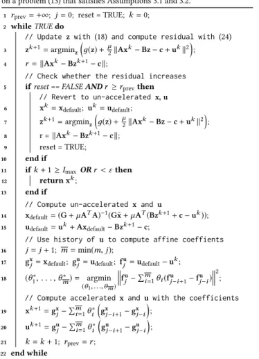
Fig. 4. For the simulation of a discretized flag with hard constraints that limit its strain, our accelerated solver convergences faster than an ADMM solver. Here the color-coding shows the deviation from the deformation gradient singular values from their prescribed range. Using the same computational budget to compute a frame, the results with our solver satisfy the strain limiting constraints better.

variable range. In the following, for all physical simulation and

geometry optimization problems, we setato the average edge length of the initial discretized model. For image processing problems, we

simply seta=1. For the choice of parameterm, similar to [Peng et al. 2018] we observe that a largemtends to improve the reduction of iteration count but increases the computational overhead per

iteration (see Fig. 2). We choosem=6 by default.

4.1 Physical simulation

Overby et al. [2017] performed physical simulation via the following

optimization problem:

min

x,z f(x)+д(z)

s.t.W(z−Dx)=0, (28)

Herexis the node positions of the discretized object,f(x)is a mo-mentum energy of the form (14) withGbeing a scaled mass matrix, Dxcollects the deformation gradient of each element,д(z)is the elastic potential energy, andWis a diagonal scaling matrix that improves conditioning. This problem is solved in (28) using ADMM

with thex-z-uiteration. As it satisfies the assumptions in Proposi-tion 3.1, we apply Anderson acceleraProposi-tion to variablezaccording to Algorithm 3. Our method is implemented based on the source code

released by the authors of [Overby et al. 2017]2. Fig. 2 compares the simulation performance on three elastic bars subject to horizontal

external forces on their two ends. We use the same material stiffness

for all bars, and a different elastic potential energy model for each

bar (corotational, StVK and neo-Hookean, respectively). We apply

the original solver and our solver with differentmvalues to the same problem for a particular frame, and plot their normalized combined

residuals and normalized forward residuals through the iterations.

The methods are compared on two types of material stiffness (“soft

rubber” and “rubber” as defined in the code from [Overby et al.

2017], with the latter one being stiffer). Our method decreases both

residuals much faster than the original ADMM solver for each

stiff-ness settings. Moreover, these two residuals are highly correlated,

which demonstrates the effectiveness of using the forward residual

to verify accelerated iterates according to Proposition 3.2. On the

2

https://github.com/mattoverby/admm- elastic

rubber models, we also evaluate the performance of the general

ap-proach in Algorithm 1 that accelerateszandutogether. We can see that acceleratingzalone leads to a faster decrease of the combined residual. One possible reason is that Algorithm 3 explicitly enforces

the compatibility condition (21), so that the acceleratedzand the recoveredualways correspond to a valid intermediate value for a certain ADMM iterate sequence. This property does not hold for

the general approach, since it only performs affine combination to

obtain the acceleratedzandu, which is more akin to finding a new initial value for an ADMM sequence. In Fig. 3, we use the same soft

rubber simulation problem to compare our method with existing

ADMM acceleration techniques, including [Goldstein et al. 2014]

and [Kadkhodaie et al. 2015] which combined Nesterov’s

acceler-ation scheme with a restarting rule based on combined residual,

as well as over-relaxation [Eckstein and Bertsekas 1992] with a

re-laxation parameterα ∈ [1.5,1.8]as explained in [Boyd et al. 2011, §3.4.3]. As [Goldstein et al. 2014; Kadkhodaie et al. 2015] rely on the

convexity of the problem, they are ineffective for this non-convex

problem and in fact increases the computational time. Although

over-relaxation speeds up the decrease of residual, it achieves less

acceleration than our method.

The solver in [Overby et al. 2017] allows enforcing hard

con-straints on node positions. Our method can be applied in such cases

as well. In Fig. 4, we simulate the movement of a triangulated flag

under the wind force. Withinд(z), the elastic potential energy for each triangle is defined as the squared Euclidean distance from its

deformation gradient to the closest rotation matrix. In addition,д(z) contains an indicator function term for the strain limit of each

trian-gle that requires all singular values of the deformation gradient to

be within the range[0.95,1.05]. Due to such hard constraints forz, we cannot apply our method to thex-z-uiteration (see Remark 3.1). Instead, we adopt thez-x-uiteration and apply Algorithm 4 to ac-celerateualone, because the iteration satisfies the assumptions in Proposition 3.3. We compare the original ADMM solver with our

ac-celerated solver withm=6. To this end, we first apply our solver to compute a simulation sequence, and then re-solve the optimization

problem using the original ADMM solver. Fig. 4 plots the

(11)

Normalized Forward Residual

Frame 200

Frame 70 Frame 300

#V: 962, #Tets: 3221

Fig. 5. Simulation of a falling horse, with hard constraints on node positions that prevent them from penetrating the static objects. Our method achieves faster convergence than ADMM, as shown by the plots of normalized for-ward residual for three frames.

see a faster decrease of the residual using our solver. In addition,

for these three frames we take the results from both solvers within

the same computational time, and use color-coding to illustrate the

maximum deviation of its deformation gradient singular values from

the prescribed range on each triangle. We can see that our solver

leads to better satisfaction of the strain limiting constraints.

Hard constraints are also used in [Overby et al. 2017] to handle

collision between objects. In Figs. 5 and 6, we apply our method in

such scenarios. Here an elastic solid horse model falls under gravity

and collides with static objects in the scene. In [Overby et al. 2017],

this is handled by enforcing hard constraints onxthat prevent the nodes from penetrating the static objects. As this would reduce the x-update step to a time-consuming quadratic programming problem, [Overby et al. 2017] linearizes the constraints and solve the resulting

linear system. However, with such modification it is no longer an

ADMM algorithm. Therefore, we apply the constraints onzinstead and solve the problem usingz-x-uiteration, with acceleration ac-cording to Algorithm 4. Figs. 5 and 6 plot the normalized forward

residual for computing certain frames in the simulation sequence,

showing a faster decrease of the residual with our method.

4.2 Geometry processing

We also apply our method to an ADMM solver for mesh optimization

subject to both soft and hard constraints based on [Deng et al. 2015].

The input is a mesh with vertex positionsx, soft constraintsAix∈ C_i (i ∈ S), and hard constraintsA_jx ∈ C_j (j ∈ H). Here each reduction matrixAi andAj selects vertex positions relevant to the constraint and (where appropriate) compute their differential

coordinates with respect to either their mean position or one of the

vertices. [Deng et al. 2015] introduce auxiliary variablesz_i ∈ C_i

Frame 20

Frame 275

#V: 962 #Tets: 3221

Fig. 6. The same simulation of a falling horse as in Fig. 5, with more complex arrangement of static objects. Our acceleration approach remains effective.

(i∈ S) andz_j ∈ C_j (j∈ H) to derive an optimization problem

min x,z 1 2 ∥L(x−x˜)∥2+ Õ i∈S wi 2 ∥Aix−zi∥2 +σC_i(zi) +Õ j∈H σC_j(zj) s.t.A_jx−z_j =0, ∀j∈ H. (29)

Here∥L(x−x˜)∥2is an optional Laplacian fairing energy for the vertex positions and/or for their displacement from initial positions,

whereas∥A_ix−z_i∥2penalizes the violation of a soft constraint with a user-specified weightwi. This problem is solved in [Deng et al. 2015] using the augmented Lagrangian method (ALM), where each

iteration performs multiple alternate updates ofzandxfollowed by a single update ofu, using the same formulas as (6). Wu et al. [2011] pointed out that it is more efficient to perform only one alternate

update of primal variables per iteration, in which case ALM reduces

to ADMM. Therefore, we solve the problem using ADMM with the z-x-uiteration, and apply the general approach in Algorithm 2 for acceleration because the target function is not separable.

In Fig. 7, we apply our method withm =6 to the wire mesh

optimization problem from [Garg et al. 2014]. The input is a regular

quad mesh subject to the following constraints:

• Hard constraints: all edges have the same lengthl; within a face, each angle formed by two incident edges is in the range[π

4, 3π

4 ].

• Soft constraint: each vertex lies on a given reference surface. The mesh is optimized without the Laplacian fairing term, i.e.,L=0. Our method leads to a faster decrease of the combined residual with

(12)

Edge length error

0 0.0008

Target Mesh

ADMM Our method

Initial Mesh

#V: 230400 #F: 229440

Fig. 7. Our method accelerates an ADMM solver for wire mesh optimization, as shown by the normalized combined residual plots. We also show two results computed using ADMM and our accelerated solver within the same computational time (indicated in the bottom-right plot), and evaluate their violation of the angle constraints and edge length constraints using the error metrics in Eq.(30). Our result satisfies these constraints better.

0 0.1

Reference surface distance

angle & edge penalty = 100 angle & edge penalty = 10000 angle & edge penalty = 1000000 ADMM penalty = 1000 ShapeUp + Anderson Acceleration Our method Target Mesh Initial Mesh

#V: 230400 #F: 229440

Fig. 8. Comparison of wire mesh optimzation results using our accelerated ADMM solver and an accelerated quadratic penalty method as described in [Peng et al. 2018]. The error metricEis the sum of squared distances from the mesh vertices to the reference shape, and the color-coding illustrates the distance for each vertex. Although the quadratic penalty method can improve satisfaction of the angle and edge length constraints with a larger penalty weight, this leads to greater deviation from the reference shape.

respect to both the iteration count and the computational time. We

also evaluate the violation of hard constraints using the following

error metrics for angleαand edge lengthe:

ξ(e)=|e−l| l , γ(α)=        π 4 −α ifα< π 4, α−3π 4 ifα> 3π 4 , 0 otherwise. (30)

The data and color-coding in Fig. 7 show that within the same

computational time, the result from our method satisfies the hard

constraints better than the original ADMM.

Besides ADMM, another popular approach for enforcing hard

constraints is the quadratic penalty method, which replaces the

original constrained problem by an unconstrained problem with

quadratic terms in the target function to penalize the violation of

hard constraints [Nocedal and Wright 2006]. Fig. 8 compares the

effectiveness of these two approaches in enforcing hard constraints

while decreasing the original target function. For the quadratic

penalty method, we use ShapeUp [Bouaziz et al. 2012] with

An-derson acceleration as described in [Peng et al. 2018], and solve

three problem instances with different penalty weights for hard

(13)

Target Mesh Initial Mesh Optimized Mesh

Our method

ADMM ₀ _0.005

Planarity error

#V:2908, #F:2825

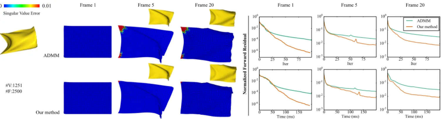
Fig. 9. PQ mesh optimization using our accelerated solver convergences faster than ADMM, and achieves better satisfaction of the planarity constraints within the same computational time (highlighted in the plot in bottom right).

full convergence for comparison. We can see that although a larger

penalty weight for hard constraints improves their satisfaction, it

also leads to relatively less penalty and greater violation of the soft

constraints. In particular, with a large penalty weight to satisfy the

hard constraints to a similar level as ADMM, the result from the

quadratic penalty method deviates much more from the reference

surface than ADMM. It shows that ADMM is more effective in

sat-isfying hard constraints without compromising the minimization of

the target function, and our method further improves its efficiency.

In Figs. 1 and 9, we apply our method to planar quad mesh

opti-mization, a classical problem in architectural geometry [Liu et al.

2006]. The input is a quad mesh subject to the following constraints:

•Hard constraint: vertices within each face lie on a common plane. •Soft constraint: each vertex lies on a given reference surface. Following [Bouaziz et al. 2012], the reduction matrix for each hard

constraint represents the mean-centering operator for the vertices

on a common face. The target function includes a Laplacian fairness

energy and a relative fairness energy for the vertex positions, as

described in [Liu et al. 2011]. We measure the planarity error for

each faceF of a given mesh using the metricdmax(F)/e, where

dmax(F)is the maximum distance from a vertex ofF to the best

fitting plane of its vertices, andeis the average edge length of the mesh. In both Fig. 1 and Fig. 9, our method accelerates the decrease

of the combined residual, producing a result with lower planarity

error than the original ADMM within the same computational time.

4.3 Image processing

In Fig. 10, we apply our method to the ADMM solver from the

ProxImaL image optimization framework [Heide et al. 2016]. We

compare our method with the original solver on the following

prob-lem that computes a deconvoluted imagexfrom an observation

imagefwith Gaussian noise and a convolution operatorK: min x,z λ1∥z1−f∥ 2+λ 2∥z i,j 2 ∥ s.t.Kx=z1, (∇x)i,j =z i,j 2 ∀i,j, (31)

where(∇x)_i_,_j is the image gradient ofxat pixel(i,j). This is solved in [Heide et al. 2016] using ADMM with thex-z-uiteration, and we accelerate it using Algorithm 1 withm=6. We modify the source code of the ProxImaL library3to implement our accelerated solver, and use conjugate gradient to solve the linear systems in the update

steps. Fig. 10 shows that our method requires less computational

time and lower iteration count to achieve the same residual value.

Finally, in Fig. 11, we accelerate the ADMM solver used by the

Coded Wavefront Sensor in [Wang et al. 2018] for computing the

observed wavefront from a captured image. The wavefrontxis

computed by solving an optimization problem

min

x,z λ∥∇x∥ 2+д

(z) s.t.∇x=z, (32)

wherezis an auxiliary variable for image gradient, andд(z)is a qua-dratic term that measures the consistency between the wavefront

and the captured image. From the general condition presented in

Appendix E.1, we know that in each iteration the dual variableuk can be represented as a function ofzkvia Eq. (49). Therefore, we apply Anderson acceleration tozalone. Moreover, asд(z)is qua-dratic, Eq. (49) implies thatzkandukare related by a linear map. Thus we use the historyzto compute the affine combination coeffi-cients for Anderson acceleration, and apply them to bothzanduto derive the acceleratedzand its compatibleu, similar to Algorithm 4. We modify the source code released by the authors of [Wang et al.

2018]4to implement our accelerated solver. Fig. 11 compares the normalized combined residual plots between the two solvers, using

a test example provided in the released source code. Compared to

the original ADMM, our method leads to a significant reduction of

computational time and iteration count for the same accuracy. Also

included in the comparison is the GMRES acceleration for ADMM

3

https://github.com/comp- imaging/ProxImaL 4

(14)

Observation Ground truth Result

Fig. 10. Our method accelerates the ADMM solver in [Heide et al. 2016] for the deconvolution of a512×512image with Gaussian noise using Eq.(31).

The given convolution operatorKis visualized in the bottom right of the observation image.

proposed in [Zhang and White 2018], which is designed

specifi-cally for strongly convex quadratic problems. Following [Zhang and

White 2018], we restart GMRES every 10 iterations to reduce

com-putational cost. As a general method, our approach is outperformed

by GMRES acceleration, but only by a small margin.

5 CONCLUSION AND FUTURE WORK

In this paper, we apply Anderson acceleration to improve the

con-vergence of ADMM on computer graphics problems. We show that

ADMM can be interpreted as a fixed-point iteration of the second

primal variable and the dual variable in the general case, and of only

one of them when the problem has a separable target function and

satisfies certain conditions. Such interpretation allows us to directly

apply Anderson acceleration in the former case, and further reduce

its computational overhead in the latter case. Moreover, for each

case we propose a simple residual for measuring the convergence,

and use it to determine whether to accept an accelerated iterate. We

apply this method to a variety of ADMM solvers in graphics, with

applications ranging from physics simulation, geometry

process-ing, to image processing. Our method shows its effectiveness on all

these problems, with a notable reduction of iteration account and

computational time required to reach the same accuracy. On the

theoretical front, we also prove the convergence of ADMM for a

common non-convex problem structure in computer graphics

un-der weak assumptions. Our work addresses two main limitations

of ADMM especially on non-convex problems, which will help to

expand its applicability in computer graphics as a versatile solver for

optimization problems that are potentially non-smooth, non-convex,

and with hard constraints.

One limitation of our method is that it can be less effective for

ADMM solvers with very low computational cost per iteration. In

this case, the overhead of Anderson acceleration can cause a large

relative increase of computational time, which partly cancels out

the speedup gained from the reduction of iteration count. One such

Ground Truth Result ADMM_{Ours m=1}

Ours m=4 Ours m=3 Ours m=2 Ours m=5 Ours m=6 GMRES

Fig. 11. Our method accelerates the ADMM solver in [Wang et al. 2018] for computing the observed wavefront from a captured image, and achieves similar performance as the specialized GMRES acceleration [Zhang and White 2018] despite being a general acceleration technique.

example is Fig. 12, where we apply our method to the ADMM solver

in [Tao et al. 2019] for correcting a vector field into an integrable

gradient field of geodesic distance. Although our method reduces the

number of iterations, its large relative overhead actually increases

the computational time for achieving the same residual.

Our experiments show that Anderson acceleration is effective in

reducing the number of iterations, but we do not have a theoretical

guarantee for such property. This is still an open research problem,

and the only existing result we are aware of is [Evans et al. 2018],

which proves that Anderson acceleration improves the convergence

rate for linearly converging fixed-point methods if a set of strong

assumptions is satisfied. Further theoretical analysis of our method

is needed to understand and guarantee its performance.

Currently we follow the convention and set the mixing parameter β =1 for Anderson acceleration. Although it is effective in our experiments, other values ofβ = 1 can potentially improve the performance [Eyert 1996]. The optimal choice of mixing parameter

remains an open research problem, and should be explored further.

The convergence of ADMM can also be affected by the choice of

the penalty parameter and the conditioning of linear side constraints.

Recently, researchers have started to analyze the optimal choice

of penalty parameter and conditioning for ADMM, but only on

simple convex problems [Ghadimi et al. 2015; Giselsson and Boyd

2017]. Overby et al. [2017] proposed a heuristic for choosing such

parameters for non-convex physical simulation problems, but there

is still no theoretical guarantee for its effectiveness. A potential

future research is to perform such analysis on non-convex problems,

as well as how they can be used in conjunction with Anderson

acceleration to further improve convergence of ADMM.