Parallel substepping scheme for elasto-plastic finite element analysis

SCHEME

FOR ELASTO-PLASTIC

FINITE ELEMENT AN

AL YSIS

Zhongwen

Ding

B.E.

(Northeastern University, P.

R.

China)

September 1999

A thesis

submitted for the degree of Master of Engineering

of The

Australian National University

Department of Engineerin

g

This thesis contains no material which has been previously accepted for the award of any other degree or diploma in any university, institute or college, and contains no material previously published or written by another person, except where due reference

is made.

Canberra, September 1999.

Journal Papers:

Zhongwen Ding Department of Engineering Faculty of Engineering and Information Technology The Australian National University Canberra ACT 0200, AUSTRALIA.

[Jl]Z.

Ding, Dr. S. Kalyanasundaram, Dr. M. Cardew-Hall, Dr. S. Robert and Dr. L. Grosz. "Integration Algorithms for Three-dimensional Elasto-plastic Finite Element Analysis," Submitted to International Journal of Numerical Methods in Engineering, under review.

Conference Papers:

[Cl]Z. Ding, Dr. S. Kalyanasundaram, Dr. L. Grosz, Dr. M. Cardew-Hall and Dr. S. Robert, "Parallel Substepping Schemes for Elasto-Plastic Finite Element Stress Anal-ysis," The Second Australasian Congress on Applied Mechanics (ACAM 99), Feb. 10 - 12, 1999, Canberra, Australia

[C2]Z. Ding, Dr. S. Kalyanasundaram, Dr. L. Grosz, Dr. M. Cardew-Hall and Dr. S. Robert, "Application of Parallel Conjugate Gradient Method to Non-linear Problem in Solid Mechanics," International Conference on Applied Modelling and Simulation (AMS'99), Sep. 1-3, 1999, Cairns, Queensland, Australia

[C3]Z. Ding, Dr. S. Kalyanasundaram, Dr. L. Grosz, Dr. M. Cardew-Hall and Dr. S. Robert, "Development of A New Method for Solving the Initial Value Problem in Elasto-Plastic Deformation Analysis," Submitted to the 9th Biennial Computational Techniques and Applications Conference and Workshops (CTAC99), September 20-24,

1999, Canberra, Australia

[C4JZ. Ding, Dr. S. Kalyanasundaram, Dr. L. Grosz, Dr. M. Cardew-Hall and Dr. S. Robert, "Parallel Elasto-Plastic Finite Element Analysis in a Workstation Cluster Environment," Submitted to The 7th International Symposium on Structural Failure and Plasticity (IMPLAST 2000), Oct. 4-6, 2000, Melbourne, Australia

In this thesis, we present the development of the parallel algorithms for elasto-plastic analysis by using finite element method. The method is based on dividing the original

structure into a number of substructures which are treated as isolated finite element models via the interface conditions. Separate input and output files are established for each subdomain. These files are read from and written to by local copies of the program executable operating in parallel. After reading corresponding input file, each

processor generates the substructure in parallel on which it will operate without any

need for communication. During the overall solution, each processor performs identical

instructions, but on different sets of data.

We focus on the establishment of algorithms for integration of the strain and stress

relations and solution of the resulting systems of equations. We employ a parallel

sub-structure oriented preconditioned conjugate gradient method combined with minimal

residual smoothing and the diagonal storage scheme to solve the systems of equations. The solution method proposed does not require the formation of global system of

equa-tions, but computes directly the displacements for each substructure, as opposed to solving a global system of nodal equations. Throughout the analysis, each processor

stores only the information relevant to its substructure and generates the local stiffness matrix.

After the displacements are calculated a substepping scheme is used to integrate elasto-plastic stress-strain relations. The procedure outlined controls the error of the computed stress by choosing each substep size automatically according to a prescribed

tolerance. The results indicate that the combination of this substepping scheme and the stress correction which is applied at the end of integration process can increase both accuracy and efficiency significantly.

When we implement the parallel algorithms we have to address the problems of load

balancing and interprocessor communication, etc. The method we use to balance the

load is to employ different partitioning schemes. The interprocessor communication is

optimized by using a special element numbering and an optimal communication scheme.

In

this thesis we will describe the implementation in further detail and give some examples of results obtained from experimental runs via Message Passing Interface on

the Linux-Alpha workstation cluster at the Australian National University

Supercom-puter Facility. The results are designed to highlight the performance of the algorithms

developed as well as their efficiency on a parallel machine.

Working on this project has been a source of great pleasure for me. At this juncture, I would like to acknowledge the people who worked with me and helped make this project a reality.

I would like to thank the people in the Department of Engineering at the Australian National University. They have helped to create a good working environment, both academically and socially. I would especially like to thank my supervisor, Dr. Shankar Kalyanasundaram for his patience and guidance. I am most indebted to him for his support throughout the duration of this project.

I would like to thank the staff at the Australian National University Supercomputer Facility, especially Roger Brown and David Singleton for their technical advice on parallel computing, particularly with regards to the Alpha-Linux workstation cluster.

I would also like to thank Dr. Lutz Grosz and Dr. Stephen Roberts, at the School of Mathematical Science, and Dr. Mick Cardew-Hall, head of the Department of Engi-neering, for their valuable input into this project.

Most of all, I would like to thank my wife, Xiaoli, for her affectionate support, patience, and encouragement all through my education at ANU.

Contents

Declaration

Abstract

Acknowledgements

Notation

1 Introduction

1.1 The Research Problem 1.2 Literature Review

1.2.1 Integration Algorithm for Elasto-Plastic Problems 1.2.2 Parallel Elasto-Plastic Finite Element Analysis 1.3 Aims . . . .

1.4 Organisation of the thesis

2 Finite Element Elasto-Plastic Analysis

2.1 Finite Element Method . . . . 2.1.1 History of Finite Element Method

iii

V

Xll

1

1 3

3

5

5

6

8 8

8

2.1.2 General Procedures of Finite Element Method . . . . . 9 2 .1.3 Basic Formulation of Finite Element Method for Non-Linear Prob

-lem . . . . . . . . . . . . . . . . 10

2.1.4 Applications of Finite Element Method 12

2.2 The Mathematical Formulation of Elasto-Plastic Problem 2.2.1 The Yield Criterion

2.2.2 Work or Strain Hardening

Vl

12

14

2.2.5 2.3

2.4

Determination of Initial Yielding State . . . Integration Algorithms for Stress-Strain Relations 2.3.1 Conventional Method . .

2.3.2 New Substepping Scheme Overall Solution Methods 2.4.1 Iterative Methods 2.4.2 Load Increment Control 2.4.3 Convergence Criteria . .

2.5 Performance Analysis of Substepping Schemes . 2.5.1 Accuracy

2.5.2 Efficiency 2.6 Summary . . . .

3 Parallel Finite Element Analysis 3.1 Parallel Computing .

Introduction 3.1.1

3.1.2 3.1.3

The Importance of Parallel Computing . The Application of Parallel Computing 3.1.4 Issues in Parallel Computing

3.2 Parallel Finite Element Analysis

3.2.1 Generation of Element Stiffness Matrices

3.2.2 Assembly and Solution of the Global System Equations 3.2.3 Calculations of Element Characteristics

3.3 Sequential Algorithm for Equation Solution 3.3.1 Conjugate gradient method . . . . . 3.3.2 Preconditioned conjugate gradient method. 3.3.3 Minimal Residual Smoothing . . .

3.4 Finite Element Transformation Relations 3.5 Parallel Algorithms for Equation Solution

3.5.1 Parallel Preconditioned Conjugate Gradient Method 3.5.2 Parallel Minimal Residual Smoothing method

4 Implementation of Parallel Algorithms 4.1

4.2

4.3

Parallel Environment .

4.1.1 Parallel Computer Architectures

4.1.2 Message Passing Interface

4.1.3 Compiler and Debugger

Performance Evaluation

4.2.1 Run time

4.2.2 Speedup .

4.2.3 Efficiency

4.2.4 Scalability .

Sources of Parallel Overhead

4.3.1 Interprocessor Communication

4.3.2 Load Imbalance . . .

4.3.3 Extra Computation

4.4 Implementation of Parallel FE Algorithms

4.4.1 Parallel Grid Generation .

4.4.2 Special numbering scheme

4.4.3 Load Balance . . . .

4.4.4 Interprocessor Communication

4.4.5 Storage Scheme .

5 Numerical Experiments 5.1 Material Parameters .

5.2 Performance of the Algorithms and Discussion

5.2.1 Application of 3-D Shallow Cantilever Beam

5.2.2 Application of 3-D Deep Cantilever Beam

6 Conclusion

6 .1 Concluding Remarks

6.2 Future Work

Bibliography

A Runge-Kutta Methods

1-1 Program structure for elasto-plastic analysis . . . . . . . 2

2-1 Geometrical representation of the Tresca and Von Mises yield surfaces

in principal stress space[2] . . . . . . . . . . . . . . . . . . . . . . . . 15 2-2 Geometrical representation of the Mohr-Coulomb and Drucker-Prager

yield surfaces in principal stress space[2] . . . . . . . . . . . . . . . 17 2-3 Mathematical models for representation of strain hardening behaviour[2] 18

2-4 Incremental stress changes in an already yielded point in an elasto-plastic

continuum. 25

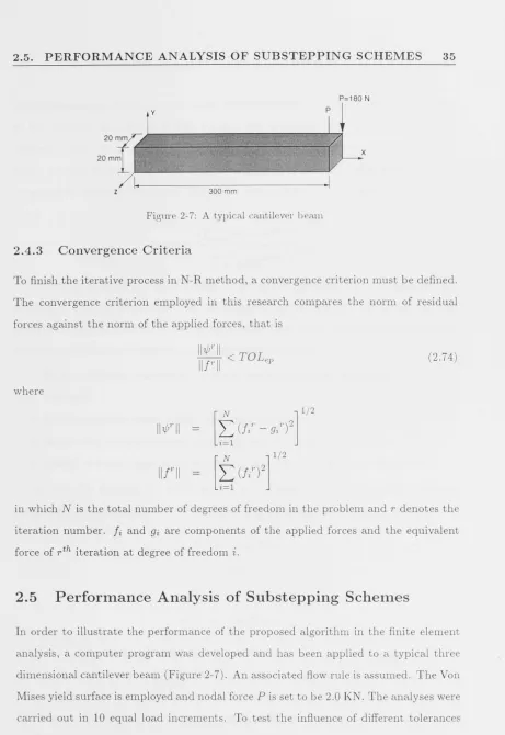
2-5 Incremental stress changes at a point in an elasto-plastic continuum at initial yield. . . . . . . . . . . . . . . . . . . . . . . 26 2-6 Refined process for reducing a stress point to the yield surface. 27 2-7 A typical cantilever beam . . . . . . . . . . . . . . . . 35 2-8 Force vs displacement curve for problem with 288 d.o.f (no strain

hard-ening). . . . . . . . . . . . . . . . . . . . . . . . . . 38 2-9 Force vs displacement curve for problem with 288 d.o.f ( a linear strain

hardening is considered). . . . . . . . . . . . . . . . . . . . . . . 39 2-10 Force vs displacement curve for problem with 432 d.o.f (no strain

hard-ening). . . . . . . . . . . . . . . . . . . . . . . . . . . . . . . . . . . . . . 40 2-11 Force vs displacement curve for problem with 432 d.o.f ( a linear strain

hardening is considered). . . . . . . . . . . . . . . . . . . . . .

3-1 Cost versus performance curve and its evolution over the decades 3-2 Element-element connectivity information. . . . .

4-1 Structure of the Linux-Alpha workstation cluster

lX

41

48

59

4-2 A three dimensional cantilever beam (8 x 8 x 32) 76 4-3 A vertical strip-wise partitioning on 4 processors 76 4-4 A horizontal strip-wise partitioning on 4 processors 76 4-5 A box-wise partitioning on eight processors . . . . 76 4-6 Sequentialization caused by sends blocking until the matching receive is

posted. The shaded area indicates the time a process is idle. 78 4- 7 Optimizaton of communication by avoiding matching delay. 78 4-8 A sparse matrix stored in the diagonal format 79

5-1 3-D shallow cantilever beam 80

5-2 3-D deep cantilever beam . 81

5-3 Parallel program structure for non-linear analysis 81 5-4 Speedup of analyses of 3-D shallow cantilever beam using horizontal

strip-wise partitioning . . . . . . . . . . . . . . . . . . . . . . . . . . 84 5-5 Efficiency of analyses of 3-D shallow cantilever beam using horizontal

strip-wise partitioning . . . . . . . . . . . . . . . . . . . . . 84 5-6 Speedup of analyses of 3-D shallow cantilever beam using vertical

strip-wise partitioning . . . . . . . . . . . . . . . . . . . . . . . . . . . . . 85 5- 7 Efficiency of analyses of 3-D shallow cantilever beam using vertical

strip-wise partitioning . . . . . . . . . . . . . . . . . . 85 5-8 Speedup of analyses of 3-D deep cantilever beam 89 5-9 Efficiency of analyses of 3-D deep cantilever beam 89

2.1 Effective stress and uniaxial yield stress levels for the yield criteria in-cluded in the elasto-plastic computer code . . . . . . . . . . . . 21 2.2 Constants defining the yield surface in a form suitable for numerical

analysis . . . . . . . . . . . . . . . . . . . . . . 22 2.3 Results of errors for problem with 288 d.o.f with different tolerances 42 2.4 Results of errors for problem with 432 d.o.f with different tolerance . 42 2.5 Total substeps needed in the overall solution for problem with 288 d.o.f

with different tolerance . . . . . . . . . . . . . . . . . . . . . 44 2.6 Total substeps needed in the overall solution for problem with 432 d.o.f

with different tolerance . . . . . . . . . . . . . . . . . . . . . . 44 2.7 CPU time (seconds)spent on computation of stress-strain relation for

problem with 288 d.o.f with different tolerance . . . . . . . . . . . . . . 45 2.8 CPU time (seconds) spent on computation of stress-strain relation for

problem with 432 d.o.f with different tolerance . . . . . . . . . . . 45

3.1 PCG algorithm with MR smoothing . . . . 57

3.2 Parallel Substructure Preconditioned Conjugate Gradient Algorithm

com-bined with MR Smoothing . . . . . . . . . . . . . . . . . . . . . . . 65

5.1 Substructure of horizontal partitioning scheme for 3-D shallow beam 82 5.2 Substructure of vertical partitioning scheme for 3-D shallow beam 83 5.3 Substructure of horizontal partitioning scheme for 3-D deep beam 88

Notation

F pe E H

H'

Q N D

Dep

B

Ji

J~

_1,

Ke,K

C T Ts Tp !::l.T A

w

WP R

s

E

yield function

equivalent nodal forces

Young's modulus

linear hardening parameter

derivative of the hardening function

plastic potential

shape functions

elastic matrix

elasto-plastic matrix

elastic strain matrix

stress invariants

invariants of the deviatoric stresses

stiffness matrix (element/global)

preconditioning matrix

time

serial run time

parallel run time

substep size

transformation matrix

potential energy of loads

total plastic work

residual in domain

speedup

efficiency

a

r

p

C

X, Xe

8d

8u

f

b E .6.c: .6.Ee .6.c:p 8c: Ep ,\ V K, (J" .6.0" O"e 0 O"y

a-er

.6.T </> \JI

flow vector

residual

direction vector

cohesion parameter

displacement vector (global/ element)

virtual displacement

internal displacement

applied forces

distributed loads/unit volume

strain vector

strain increment

elastic strain increment

plastic strain increment

virtual strain

effective plastic strain

plastic multiplier

Poisson's ratio

hardening parameter

stress vector

stress increment

trial stress

uniaxial yield stress

effective stress

stress, finite element approximation

shear stress increment

angle of internal friction

Chapter

1

Introduction

1.1

The Research Problem

The finite element method is now firmly accepted as a powerful general technique for

the numerical solution of a variety of problems encountered in engineering. Among its

many applications, the finite element analysis of elasto-plastic behaviour is a subject of

great importance for fundamental and practical reasons. Elasto-plastic modelling can

help us make a more complete use of the strength resources of solids and leads to an

efficient method for calculating details of machines and structures as regards to their

load-bearing capacity. However, as increasingly large-scale three-dimensional finite

element models are currently being used in various disciplines for realistic simulation

of engineering problems, the use of such complex models raises a number of questions

in relation to accuracy and efficiency. A great deal of effort has therefore been invested

in developing algorithms that can quickly and accurately solve the large-scale problems

encountered in practice.

The analysis of nonlinear elasto-plastic problems must proceed in an incremental

manner since the solution at any stage may not only depend on the current

displace-ment of the structure, but also on the previous loading history. A simplified depiction

of sequential program structure is given in Figure 1-1. The diagrams on the right-hand

side of Figure 1-1 indicates the computing time spent on different parts of the

pro-gram. For large, three-dimensional problems the overall CPU time is dominated by the

solution of systems of equations. The only other parts of the program that require sig

-nificant computational resources are the computation of the stiffness matrices for each

INCREMENTS THE APPLIED LOADS

CALCULATE THE ELEMENT STIFFNESS' ~

SOLUTION OF SYSTEM OF EQUATIONS

CALCULATE STRAINS AND STRESSES

NO

837 D.O.F 8325 D.O.F

Figure 1-1: Program structure for elasto-plastic analysis

element and evaluation of strains and stresses for each integration point. For large-scale

three-dimensional problem, the integration of strain-stress relations and the solution of

equations form two important stages in finite element elasto-plastic analysis.

As shown in Figure 1-1, two primary loops are necessary to increment the applied

loading and to iterate the solution until convergence occurs. If the load increment is

too small, the total number of iterations involved in the overall solution will increase

dramatically. The computational time will increase as well since during each iteration

a linear system of equations has to be solved which is the most time-consuming part in

the overall solution of large-scale three-dimensional applications. On the other hand,

in each load increment, the inaccurate integration of constitutive equations may cause

the prolonged iteration to converge. This indicates that efficient algorithms for

elasto-plastic finite element analysis are essential to allow greater load increment and to

decrease the total number of iterations needed to converge. Therefore, one of the key

factors of an efficient algorithm is that the constitutive law be integrated accurately.

The conventional method for integrating elasto-plastic stress-strain relations used

simple Euler scheme and divided the integration process into a number of equal

sub-steps. However, this technique requires that load increments be kept small so that the

stresses computed at the end of integration procedure do not deviate too far from the

yield surface. For the applications with relative large load increments, the computed

stresses may not satisfy the yield criterion after integration process. Therefore, a

[image:17.535.30.501.35.721.2]

1.2.

LITERATURE REVIEW

3

frequently. Since the stress correction applied at the end of integration process does

not affect the accuracy significantly, it is difficult to ensure that the strain-stress

rela-tion can be integrated with adequate accuracy. Therefore, it is necessary to develop a

integration algorithm which can control the errors in the integration process.

It is well-known that most of the computations involved in the finite element

anal-ysis are carried out at the element level. Consequently, these operations can be carried

out in parallel independent of each other. However, after the elemental calculations

have been achieved, the calculation of the displacements can become a bottleneck for

parallel implementation, since the global matrix and vector need to be assembled at

this stage. It would be very natural, especially from a parallel processing viewpoint, if

the formation of the global equations could be avoided, that is, the selected numerical

algorithm could be operated at the element or substructure level. Generally, this is

the case for iterative solution methods based on matrix-vector. Also, since the

itera-tive method employed in the finite element analysis does not change the structure of

stiffness matrix, it maintains its sparsity. Hence, the computational costs and memory

space associated with zero fill-ins can be greatly reduced by using a suitable storage

scheme. So development of a efficient parallel algorithm is another important task for

this research work.

1.2

Literature Review

1.2.1

Integration Algorithm for

Elasto-Plastic Problems

In the past 20 years, significant advances have been made in the development and

application of numerical methods to the solution of elasto-plastic problems. It is well

known that one of the simplest numerical schemes, which has been used widely in

finite element codes, is the first order Euler algorithm. This has the advantage of being

straightforward but also has the disadvantage of being accurate only for very small time

steps. To avoid this shortcoming, it is usual to subdivide the particular time step into

a number of smaller substeps and apply the Euler schemes to each of these[l, 2]. This

partially overcomes the disadvantage of the Euler approach but usually leads to a set

of stresses which do not lie precisely on the yield surface at the end of each time step.

computation, it is usual to apply some form of correction[3] to the stresses to restore

them to the yield surface. Since the stress correction is normally applied at the end of integration process, it does not significantly affect the accuracy. [4]

A number of new integration algorithms therefore were developed with an aim to

control the error in the integration process[4]-[26]. Wissmann and Hauck[4] developed a algorithm with an aim to control the errors in the integration process by using

Richard-son extrapolation to selected number of fixed size substeps. Polat and Dokainish[5] took

into account the change in the plastic flow direction due to continuing plastic deforma-tion and an automatic subincrementation scheme has been proposed for further

accu-racy improvement. Eterovic and Bathe[6] presented a hyperelastic-based large strain formulation using the product decomposition of the deformation gradient into elastic

and plastic parts for metal plasticity. Pezeshk and Camp[7] have proposed an

integra-tion method based on a Modified Trapezoidal rule Method. The resulting algorithm is

extremely simple to use. However, it is conditionally stable. It is especially worthy not-ing that Sloan[8, 9] used a substepping scheme to integrate the stress-strain relations.

The substep size is decided by comparing a prescribed tolerance with an estimate of the error of the integrated stress increment. This error estimate is obtained by

compar-ing the estimated stress increments which result from two integration procedures with truncation errors of different order. Two substepping schemes are recommended in [8],

which are based on modified Euler method and the fifth order Runge-Kutta-England,

respectively. The application of a smooth rigid strip footing resting on an ealsto-plastic

soil mass indicated that no form of the stress correction is required. However, Gens

and Potts suggested in [10] that, the deviation from the yield surface is directly related

to the level of error in computed stresses and it is practically independent of the

1.3. AIMS 5

1.2.2

Parallel Elasto-Plastic Finite Element Analysis

At present, the parallel algorithms for linear analyses have made considerable

head-way. However, in the aspect of nonlinear analyses, wide-ranging research has not been

undertaken; Wilson and Farhat[33], Sun and Mao[34], Farhat and Crivell[35],

Shivaku-mar, Bigelow and Newman[36], Kacou and Parsons[37], Hu[38], Klaas, Kreienmeyer

and Stein[39], Feriani, Franchi and Genna[40][41] et al. have implemented such

non-linear analysis on parallel computer systems. However the integration schemes they

employed are based on the conventional finite element method in which no measure is

used to control the error in the integration process. In fact, the error in the computed stresses is very important for the non-linear elasto-plastic analysis, since large error can

cause a prolonged iteration to converge.

In parallel finite element analysis for elasto-plastic problem, solving the linearized

system of equations forms another important stage. Techniques to solve the equations

system may generally be classified into two categories, one is the direct parallel solution;

Melosh and Utku[42], Doi and Koyama[43], Noor, Kamel and Fulton[44], Farhat and

Wilson[45], Malone[46], Goehlich, Komzsik and Fulton[47] et al. have all conducted

some research work in this field. The other is the iterative solution; Hughes, Levit

and Winget[48], Law[49], King and Sonnad[50], Carter, Sham and Law[51], Johnsson

and Mathur[52], Kumar, Grama, Gupta and Karypis[53] et al. have proposed different

iterative algorithms. The main virtue of direct parallel solution is the strong

numer-ical stability, but the weak point is that synchronous control must be introduced in

most cases. The main advantage of iterative parallel solution is that the excessive

syn-chronous control steps can be avoided, but there are some problems in the numerical

stability of the algorithm. The direct parallel algorithms are commonly developed from

the substructuring techniques or the synchronous control solutions of the finite element

equations. The iterative parallel algorithms are generally based on preconditioned

con-jugate gradient PCG) or Jacobi methods.

1.3

Aims

The aim of this research project is to research methods for developing an

finite element solution procedure with relevance to elasto-plastic modelling.

In order to develop the above framework the following important areas needed to

be researched:

• Accurate integration algorithm for strain-stress relationships.

• Efficient parallel algorithm for the solution of linear system of equations. • A suitable storage scheme for overall solution.

• Implementation of the developed parallel algorithms on the computer platforms

to achieve optimal performance.

With these thoughts in mind, we will develop a substepping scheme for elasto-plastic

stress integration process. The resulting algorithm can be applicable to a general type

of constitutive law and controls the error in the integration process by adjusting the size

of each substep automatically in accordance with the behaviour of the constitutive law.

For the equation solution, a combination of preconditioned conjugate gradient method with minimal residual smoothing will be employed. In the resulting parallel algorithm, the formation of the global system_ matrix is not performed, but the displacements

for each substructure are computed directly, as opposed to solving a global system of

nodal equations. The resulting algorithms will be tested on a workstation cluster. To

obtain an optimal performance, a diagonal storage scheme will be employed. Different

partitioning scheme will be used with an aim to obtain better load balance. Also, a

special numbering of the elements and an optimized communication scheme are adopted

in this research work.

1.4

Organisation of the thesis

This thesis chronicles our experience with parallel finite element analysis in the context

of non-linear elasto-plastic finite element simulation over the past two years. An outline

of this thesis is as follows.

Chapter 2 commences with a brief review of finite element method and its

appli-cation to nonlinear problem. For elasto-plastic applications to be considered, basic

theoretical formulations are developed in a form suitable for numerical solution.

1.4. ORGANISATION OF THE THESIS

7

an advanced substepping scheme will be introduced and its advantages will be

demon-strated. The overall solution method will also be presented for completeness.

Chapter 3 deals with the development of parallel algorithm for the solution of linear

system of equations. Both sequential algorithm and parallel algorithm are outlined. A finite element transformation relations is introduced which forms a bridge between sequential algorithm and parallel algorithm.

In Chapter 4, we present an introduction of parallel environment which is used in

this research work. Some of the important issues in implementation of the parallel algorithms on the chosen parallel machine are also reviewed.

Chapter 5 conducts application of the resulting parallel algorithms to a

three-dimensional elasto-plastic analysis. The speedup, efficiency and scalability will be studied.

Chapter 6 summarises the main conclusions of the study and provides some

Finite Element Elasto-Plastic

Analysis

A general introduction of finite element method is presented in this chapter. Basic

theoretical formulations for elasto-plastic problems are developed in a form suitable

for numerical solution. Based on it, a conventional method for integrating the

strain-stress relations will be discussed. An advanced substepping scheme will be developed

and its performance will be given. For a better understanding of the performance of substepping scheme, the overall solution methods which are employed in the finite

element code will be briefly introduced.

2.1

Finite Element Method

The finite element method is a numerical analysis technique for obtaining approximate

solution to a wide variety of engineering problems. Although originally developed to

study the stresses in complex airframe structures, it has since been extended and applied

to the broad field of continuum mechanics. Because of its diversity and flexibility as

an analysis tool, it is receiving much attention in engineering schools and in industry.

2.1.1

History of Finite Element Method

Finite element analysis was first developed in 1943. During its early development for stress analysis problems the method relied heavily on a physical interpretation in which

the structure was assumed to be composed of elements physically connected only at

2.1. FINITE ELEMENT METHOD

9

a number of discrete nodal 'points. Later the application of the method to structural mechanics problems was developed through the use of the principle of virtual work and energy methods. The method was then generalised and its wider mathematical roots were recognised. It was shown that finite elements could be applied to any mathematical problem for which a variational functional existed. More recently, finite

element solutions have been developed which are based on the well known, classical techniques known as "weighted residual methods". Since the 1970's the rapid growth in engineering usage of computer technology has a significant effect upon the acceptance

of the finite element method. In fact the finite element method is now firmly established as an engineering tool of wide applicability. One of the principal advantage of the finite

element method is the unifying approach it offers to the solution of diverse engineering problems.

2.1.2

General Procedures

of Finite Element Method

Regardless of the approach used to different applications, the solution of finite element method always follows an orderly step-by-step process. To summarize in general terms how the finite element method works we will succinctly list these steps. These well-defined modules are a base of parallel finite element analysis.

l. Discretize the continuum. The first step is to divide the continuum or solution

region into elements. A variety of element shapes is available for different analysis.

2. Select interpolation functions. The next step is to assign nodes to each ele-ment and then choose the type of interpolation function to represent the variation

of the field variable over the element.

3. Find the element properties. Once the finite element model has been

estab-lished, we are ready to determine the matrix equations expressing the properties of the individual element.

4. Assemble the element properties to obtain the system equations. To find the properties of the overall system modelled by the network of elements we must "assemble" all the element properties.

values of the field variable. Technique to solve this equations system may generally

be classified into direct and iterative methods.

6. Calculate the element characteristics. Normally we use the solution of the system equations to calculate other important parameters, such as strains,

stresses, ... etc.

2.1.3

Basic Formulation of Finite Element Method

for Non-Linear

Problem

For any numerical approach an approximate solution is attempted by assuming that

the behaviour of the continuum can be represented by a finite nurn.ber of unknowns.

As previously mentioned in the finite element method the continuum is divided into

a series of elements which are connected at a finite number of points known as nodal

points.

For structural applications at least, the governing equilibrium equations can be

obtained by the principle of virtual work[2]. Consider the solid, in which the internal

stresses a, the distributed loads/unit volume b and external applied forces

f

form an equilibrating field, to undergo an arbitrary virtual displacements pattern 5d which results in compatible strains

5c

and internal displacements 5u. Then the principle of

virtual work can be expressed as

l

(OET

CY - OuTb)dO. - OdT

f

= 0

(2.1)

In the finite element displacement method, the displacement is assumed to have

un-known values only at the nodal points, so that the variation within any element 1s

described in terms of the nodal values by means of interpolation functions. Thus

ou

=

N5d (2.2)

where N is the set of interpolation functions termed the shape functions. The strains

within the element can be expressed in terms of the element nodal displacements as

5c

=

Bod (2.3)

where B is the strain matrix generally composed of derivatives of the shape functions.

Then the element assembly process gives

2.1.

FINITE ELEMENT METHOD

11

where the volume integration over the solid is the sum of the individual element

con-tributions. Since this expression must be hold true for any arbitrary 5d value

l

BT adD - f -

l

NTbdD

=

0 (2.5)

For the solution of nonlinear problems which will be described in the following,

Equa-tion 2.5 will not generally be satisfied at any stage of the computation, and

'¥

=

l

BT adD -

(1

+

l

NTbdD) =/= 0 (2.6)

where '1! is the residual force vector. For an elasto-plastic situation the material stiffness

is continually varying, and instantaneously the incremental stress/strain relationship is given

'6.a

=

Dep'6.E (2.7)

For the purpose of evaluating the material tangential stiffness matrix Kr at any stage,

the incremental form of (2.6) must be employed. Thus, within an increment of load we

have

6.

1¥

=

l

BT 6.adD - ( 6.f

+

l

NT 6.bdD) Substituting for '6.a from Equation 2.7 results in

6. '¥

=

Kr6.d - ( 6.f

+

l

NT 6.bdD)

where

[Kr]=

l

BTDepBdD

(2.8)

(2.9)

(2.10)

is termed the element stiffness matrix. The final system of equations that results from the above approximation is of the form

[K]

{x}

=

{J}

(2.11)

where the global stiffness matrix

[K]

is really a collection of elemental stiffness matrices

N

[K]

=

I)x

(e)]

(2.12)

e=l

These equations are then solved by any standard technique to yield the nodal displace-ments. After this, the stresses within each element can then be calculated from the

2.1.4

Applications of Finite Element

Method

The range of possible applications of the finite element method extends to all

engineer-ing disciplines, although civil and aerospace engineers concerned with stress analysis

are the most frequent user of the method. Its applications mainly range from the stress

analysis of solids to the solution of acoustical, neutron physics and fluid dynamics

problems. Indeed the finite element process is now established as a general

numeri-cal method for the solution of partial differential equation systems, subject to known

boundary and/ or initial conditions.

For linear application, at least, the technique is widely employed as a design tool.

Similar acceptance for nonlinear applications is dependent on two major factors. Firstly,

in view of the increased numerical operations associated with nonlinear problems,

con-siderable computing power is required. Although developments of high-speed digital

computers in the last decade or so met this need to some extent, in fact, some

prob-lems can still be classified as 'difficult' to solve, even for modern vector supercomputers.

Parallel processing may be the most promising way to reduce the computation time as

new generations of parallel computers are rapidly emerging. Secondly, before the finite

element method can be used in design, the accuracy of any proposed solution technique

must be proven. Although the development of improved element characteristics and

more efficient nonlinear solution algorithms and the experience gained in their

appli-cation to engineering problems have ensured that nonlinear finite element analyses can

now be performed with some confidence, efficient and accurate algorithms for parallel

processing are still urgently needed. These suitable algorithms are essential to allow

greater load step and to decrease the total amount of computation. Hence the effort on

trying to remove the barriers to the common use of nonlinear finite element techniques

will never end.

2.2

The Mathematical Formulation of Elasto-Plastic

Prob-lem

In this section, we consider the elasto-plastic stress analysis of solid which conforms

to three-dimensional conditions. The basic laws governing elasto-plastic material

2.2. THE MATHEMATICAL FOR

MUL

AT

I

O

N OF ELASTO-PLASTIC

PROBLEM

13

the problem can be considered and to this end some concepts, such as the plastic

po-tential and the flow rule will be introduced. Only essential expressions will be provided

in this thesis and a more complete theoretical treatment can be found, for example, in

[2] and [29].

The object of the mathematical theory of plasticity is to provide a theoretical

de-scription of the relationship between stress and strain for a material which exhibits an

elasto-plastic response. In essence, plastic behaviour is characterised by an irreversible

straining which is not time dependent and which can only be sustained once a certain

level of stress has been reached. In this thesis we outline the basic assumptions and

associated theoretical expressions for a general continuum. In order to formulate a

theory which models elasto-plastic material deformation three requirements have to be

met:

• An explicit relationship between stress and strain must be formulated to describe

material behaviour under elastic conditions,i.e. before the onset of plastic

defor-mation.

• A yield criterion indicating the stress level at which plastic flow commences must

be postulated.

• A relationship between stress and strain must be developed for post-yield

be-haviour,i.e. when the deformation is made up of both elastic and plastic

compo-nents.

Before the onset of plastic yielding the relationship between stress and strain 1s

given by the standard linear elastic expression.

6..c

=

D-1

6.a (2.13)

For three-dimensional isotropic pro bl ems

{ 6.. a}

=

(

6.. a :r , 6.. a y , 6.. a z , 6.. T 1:y , 6.. Ty z , 6.. T z 1:) T (2.14)

A1

D=

sym.

where

Ai=

E(l

-

v) .

(

l+

v)(

l -

2v)'

A2 A2

0 0 0

A1

A2

0 0 0

A1 0 0 0

A3

0 0

A3

0

A3

Ev

A2

=

-(

l

+

V)

(

1 -

2v) 1

(2.16)

A - E 3

-2

(

l+v

)

in which E and v are respectively the elastic modulus and Poisson's ratio of the

mate-rials.

2.2.1

The Yield Criterion

The yield criterion determines the stress level at which plastic deformation begins and can be written in the general form[2]

(2.17)

where K is the hardening parameter. On physical grounds, any yield criterion should

be independent of the_ orientation of the coordinate system employed and therefore it

should be a function of the three stress invariants only,

Ji,h

and

h.

Experimental

observations indicate that plastic deformation of metals is essentially independent of

hydrostatic pressure. Consequently the yield function can only be of the form

(2.18)

in which

h'

and

J/

are the second and third invariants of the deviatoric stresses.

The situation is complicated by the fact that different classes of materials exhibit

different elasto-plastic characteristics. In this thesis four commonly used yield criteria

are introduced. The Tresca and Von Mises laws which closely approximate metal

plas-ticity behaviour are considered and the Mohr-Coulomb and Drucker-Prager criteria

2.2. THE MATHEMATICAL FORMULATION OF ELASTO-PLASTIC

PROBLEM 15

Space diagonal

1r plane

a1

+

a2

+

a3

Tresca

/

/ /

Figure 2-1: Geometrical representation of the Tresca and Von Mises yield surfaces in

principal stress space[2]

Tresca Yield Criterion

The Tresca yield criterion states that yielding begins when the maximum shear stress

reaches a certain value. If the principal stresses are a1, a2, a3 where a1

2::

a2

2::

a3 then yielding begins when

a1 - a3

=

Y(K) (2.19)

where Y is a material parameter to be experimentally determined and which may be a function of the hardening parameter K. By considering all other possible maximum

[image:30.528.48.481.39.727.2]

Von Mises Yield Criterion

Von Mises suggested that yielding occurs when the second invariants of the deviatoric

stresses, J2', reaches a critical value, or

1

(h')2

₌

_{k(K,) (2.20)}

in which k is a material parameter to be determined. Figure 2-1 shows the geometrical

interpretation of the Von Mises yield surface to be a circular cylinder whose projection

onto the 1r plane is a circle. A physical meaning of the constant k can be obtained

by considering the yielding of materials under simple stress states. For most metals

Von Mises' law fits the experimental date more closely than Tresca's, but it frequently

happens that the Tresca criterion is simpler to use in theoretical applications.

Mohr-Coulomb Yield Criterion

This is a generalisation of the Coulomb friction failure law defined by

T

=

c - an tan¢ (2.21)

where Tis the magnitude of the shearing stress, O-n is the normal stress, c is the cohesion

and ¢ the angle of internal friction. Again, as for the Tresca criterion, the complete

yield surface is obtained by considering all other stress combinations which can cause

yielding ( e.g. a3

S

0-1

S

0-2). In principal stress space this gives a conical yield surface

whose normal section at any point is an irregular hexagon as shown in Figure 2-2. This

criterion is applicable to concrete, rock and soil problems.

Drucker-Prager Yield Criterion

An approximation to the Mohr-Coulomb law was presented as a modification of the

Von Mises yield criterion. The influence of a hydrostatic stress component on yielding

was introduced by inclusion of an additional term in the Von Mises expression to give

1

aJi

+

(h')

2

₌

_{k' (2.22)}

This yield surface has the form of a circular cone. In order to make the Drucker-Prager

2.2.

THE MATHEMATICAL FORMULATION OF

ELASTO-PLASTIC

PROBLEM

17

0"3

I

~~D:::::;::~::b

i'/

(

I/

/;,

f/~

/

~ff/

I/

--

0"2

o

7

0"1

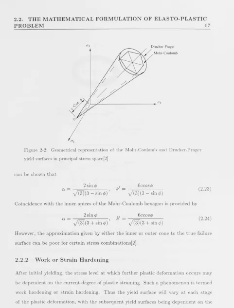
Figure 2-2: Geometrical representation of the Mohr-Coulomb and Drucker-Prager

yield surfaces in principal stress space[2]

can be shown that

2 sin¢ a= /(3)(3 - sin¢)'

k'

=

6ccos¢

/(3)(3 - sin¢) (2.23)

Coincidence with the inner apices of the Mohr-Coulomb hexagon is provided by

2 sin¢

a= /(3)(3 +sin¢)'

k'

=

6ccos¢

/(3)(3 +sin¢) (2.24)

However, the approximation given by either the inner or outer cone to the true failure

surface can be poor for certain stress combinations[2].

2.2.2

Work or Strain Hardening

After initial yielding, the stress level at which further plastic deformation occurs may

be dependent on the current degree of plastic straining. Such a phenomenon is termed

work hardening or strain hardening. Thus the yield surface will vary at each stage

of the plastic deformation, with the subsequent yield surfaces being dependent on the

plastic strains in some way. Some alternative models which describe strain hardening

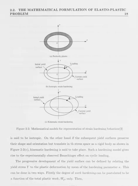
in a material are illustrated in Figure 2-3. A perfectly plastic material is shown in

Figure 2-3(a) where the yield stress level does not depend in any way on the degree of

plastification. If the subsequent yield surfaces are a uniform expansion of the original

[image:32.528.31.512.24.656.2]

Initial yield

surface

Initial yield

surface~

(a) Perfectly plastic

T

0

(b) Isotropic strain hardening

T

(c) Kinematic strain hardening

0-Current yield surface

0-Current yield surface

Figure 2-3: Mathematical models for representation of straii1 hardening hehaviour[2)

1s said to be isotropic. On the other hand if the subsequent yield surfaces preserve their shape and orientation but translate in th stress space as a rigid body as shown in Figure 2-3( c), kinematic hardening is said to take place. Such a hardening model gives

rise to the experimentally observed Bauschinger effect on cyclic loading.

The progressive development of the yield surface can be defined by relating the

yield stress Y to the plastic deformation by mean of the hardening parameter "'-· This can be done in two ways. Firstly the degree of work hardening can be postulated to be

a function of the total plastic work, Wp, only. Then,

K,

=

f

(Wp) ( 2. 25)

Alternatively K, can be related to a measure of the total plastic deforrnation termed the

effective plastic strain. Then the hardening parameter is assurn.ed to be defined as

[image:33.528.27.499.29.660.2]

2.2. THE MATHEMATICAL FORMULATION OF ELASTO-PLASTIC

PROBLEM

19

where Ep is the result of integrating the increment of the effective strain dEp over the

strain path. This behaviour is termed strain hardening. Only an isotropic hardening model will be considered in this research.

2.2.3

Elasto-Plastic Stress/Strain relations

After initial yielding the material behaviour will be partly elastic and partly plastic.

During any incremental of stress, the total strain increment may be additively decom-posed into an elastic and a plastic part, respectively

~c =~Ee+ ~Ep (2.27)

The elastic strain increment is related to the stress increment by Equation 2.13.

In order to derive the relationship between the plastic strain component and the

stress increment a further assumption on the material behaviour must be made. In particular it will be assumed that the plastic strain increment is proportional to the

stress gradient of a quantity termed the plastic potential Q, so that

~Ep

=

~A 8Q

aa

(2.28)

where ~A is a proportionality constant termed the plastic multiplier. Equation 2.28 is termed the flow rule since it governs the plastic flow after yielding. The potential Q must be a function of

h'

and

h'

but as yet it cannot be determined in its most general

form. However the relation F

=

Q

has a special significance in the mathematical theory

of plasticity, since for this case certain variational principles and uniqueness theorems can be formulated. Such assumption give rise to an associated plasticity.

When plastic yielding is occuring the stresses are on the yield surface given by

Equation 2.17. Differentiating this we can therefore write

8F

8F

8F

~F

= -

₈

~a1

+

-8

~a2

+ ... + -

8

~"'

=

0

a1 a2 "'

(2.29)

By using Equation 2.27-2.29, we obtain, after some transformation, the complete elasto-plastic incremental stress-strain relation to be

~a= Dep~E (2.30)

where

If the flow rule is assumed to be associated, then we can simply write Dep as

D ep =D- dn

=

Da (2.32)

and

T

EJF

[

EJF EJF EJF

EJF

EJF

EJF

]

a - - -

--

EJa

-

Oa

:

r' Oay' EJa

z

' OT

:1

:

y'

OTy

z'

OT

z:1:

'

(2.33)

Clearly for ideal plasticity with no hardening, H' is simply zero. When a linear

work hardening is considered, H' is obtained to be the local slope of the uniaxial

stress/plastic strain curve, which is constant and can be determined experimentally[2].

2.2.4

Alternative Form of the Yield Criterion for

Numerical

Compu-tation

For numerical computation it is convenient to rewrite the yield function in terms of

alternative stress invariants. The main advantage of this formulation is that it permits

the computer coding of the yield function and flow rule in a general form and

neces-sitates only the specification of three constants for any individual criterion. Normally

a parameter

e

(Lode angle) is used in such definition. By noting the cyclic nature of

sin(38

+

2mr) we have immediately the three possible values of sine which define the

three principal stresses. In [2], the total principal stresses are expressed as

{ a

1

} , .!. { sin (

e

+

2

t)

}

{

1 }

2(h)2

• 11

a2

=

V3

sm

e

+

3

1

0"3 sin ( 8

+

4

t)

1

(2.34)

with a1

>

0-2

>

a3 and -Tr

/6

~

e

~ 1r

/6.

The four yield criteria considered in section 2.2.1 can now be rewritten in terms of

Ii

,

h'

and 8 as follows.

The Tresca Yield Criterion

Substitute for a1 and a3 from Equation 2.34 into Equation 2.19 gives

2 , .!. [ ( 21r) ( 41r)]

V3

(

h

)

2 sin

e

+

3

-

sin

e

+

3

=

y

(

K,)

or expanding we have

1

2.2. THE MATHEMATICAL FORMULATION OF ELASTO-PLASTIC

[image:36.536.31.517.35.772.2]

PROBLEM 21

Table 2.1: Effective stress and uniaxial yield stress levels for the yield criteria included

in the elasto-plastic computer code

Uniaxial Stress level ( or equivalent

Equation No. Yield criterion ( effective stress) yield stress)

(2.35) Tresca

1

2(h')2 cos

e

Jy

(2.36) Von Mises v3(h')

!

oy

(2.37) Mohr-Coulomb ₃ lJ · 1 sm

cp

+

(J')12 /2 X ( cos 8 - sin 8 sin

cp

j

/3)

ccos ¢

1

(2.38) Drucker- Prager

aJi

+

(h')2

k'

The Von Mises Yield Criterion

There is no change in this case since this yield function depends on

h'

only. We rewrite

Equation 2. 20

1

V3(h')2

=

0-y(K) (2.36)

The Mohr-Coulomb Yield Criterion

Substitute for 0-1 and 0-3 from Equation 2.34 into Equation 2.21 results in.

iJisin¢, +

(h')l

/

2

(cos@ - ~)

=

ccos ¢ (2.37)

The Drucker-Prager Yield Criterion

There is no change for this criterion and we can write directly from Equation 2.22 that

1

aJi

+

(h')2

=

k' (2.38)

where a and k' are defined in Equation 2.23 or 2.24. The four yield criteria are

sum-marised in Table 2 .1

In order to calculate the Dep matrix in Equation 2.32, we also require to express

the flow vector a in a form suitable for numerical computation. We can always write

BF

BF 81

BF

8(J ')

112

BF ae

a T = - = - - 1 + 2

+

-80-

a11 ao-

a(

h'/

1

2

_ao-

_{ae Bo-}

(2.39)

we can then write

[image:37.526.39.505.25.520.2]

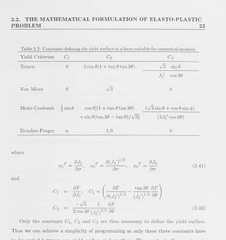
Table 2.2: Constants defining the yield surface in a form suitable for numerical analysis

Yield Criterion C1 C2 C3

-Tresca 0 2 cos 8(1 + tan

e

tan 38) _{v3 sine}

J'

₂ cos 38

Von Mises 0 v3 0

Mohr-Coulomb

!

sine cos8[(1 + tan8tan38) ( v3 sin

e

+ cos

e

sin ¢)

+sin8(tan38 - tan8)/v3] (2h' cos 38)

Drucker- Prager CY 1.0 0

where

a1T 8J1 a2T = B(h')1;2 T

oh

0(]'

_'

0(]'

'

a3 = -0(]' (2.41)

and

C1

BF

(

BF

tan3e

BF)

8J1' C2 =

a(

h')

1;2 - (

h')

1;2

ae

-/3

1

BF

C3

2cos38 (h')3/2

ae

(2.42)

Only the constants C1, C2 and C3 are then necessary to define the yield surface.

Thus we can achieve a simplicity of programming as only these three constants have

to be varied between one yield surface and another. The constants Ci are given in

Table 2.2 for the four yield criteria considered.

2.

·

2.5

Determination of Initial Yielding State

During the application of an increment of load an element, or part of an element,

may yield. All stress and strain quantities are monitored at each Gaussian integration

point and therefore we can determine whether or not plastic deformation has occurred

at such points. Consequently an element can behave partly elastically and partly

elasto-plastically if some, but not all, Gauss points indicate plastic yielding. For any

2.2. THE MATHEMATICAL FORMULATION

OF ELASTO-PLASTIC

PROBLEM

23

Within a particular load increment, the displacements increments 6.ur can be deter-mined by solving a linear system of equations. The strain increments at an integration point may be computed from the strain-displacement relations according to

L:l.Er

=

Bf:l.ur _(2.43)

where r denotes the rth iteration of current load step. Once the strains have been

determined, the elastic stress increments (i.e. the trial stress) may be calculated using

Hooke's law:

6.a/ = Df:l.cr (2.44)

and a trial stress state is obtained through

a/ = a·,·-l

+

6.a/ _{( 2 .45)}

where the subscript e denotes that we are assuming elastic behaviour. The trial stress

aer is then tested in Equation 2.17. If F

<

0, then the elasticity assumption is taken to

be valid, and a er is considered as the new stress state. Otherwise, the strain increment

is partly in an elastic path and partly in a plastic path. In order to determine the

portion of the stress which cause purely plastic yielding, we need to find a scalar a such

that

F(ar,

H)

=

0

where

ar

=

ar-1

+

(1 - a)6.a/'

A variety of schemes are available for determining scalar a. In [2], Sloan used a

Newton-Raphson iteration to compute a. It should be noted that performing iterations in the

integration scheme may lead to better results but the procedures often fails to converge.

In this thesis, a linear interpolation method is used. we rewrite Equation 2.17 in the

following form

F(a,H)

=

a- -

Y(H)

=

0 (2.46)

where

a-

and Y(H) denote the effective stress and the isotropic hardening function,

this thesis, the hardening parameter is assumed to be related to some measure of the

plastic strains. So we can write

Y(H)

in the following form:

Y(H)

=

Y(tp)

=

ay0

+

H'

tp

(2.4

7)

where ay0 _{denotes the uniaxial yield stress. Then}

a can be obtained by

F ( a

e1·,

yr-1)

a= -F(aer,

yr-1)

_

F(ar-1,

yr-1)

a~ -

yr-1

a~ - ar-1

(2.48)

where yr-l

=

ay0

+

H'

s;;-

1_{. After determining the portion of the stress increments}

which cause purely plastic yielding, we must reduce the excess stress onto the yield

surface until yield criterion and the constitutive law are satisfied.

2.3

Integration Algorithms for Stress-Strain

Relations

Once the stresses at the onset of initial yielding have been computed, the integration

of stress-strain relations requires the solution of the initial value problem given by

da

dT

=

Depflc,

TE [O, 1]

(2.49)

in which ajT=O defines the stress state which already satisfy the yield criterion, and

ajT=l defines the stress at an end of load increment or iteration. Both the conventional

integration algorithm and a substepping scheme are studied in this research.

2.3.1

Conventional Method

The crudest method for solving the system of differential equations defined by 2.49 is

the Euler algorithm. Since the Euler scheme is accurate only for very small time steps,

it is always necessary to divide the whole integration process into a number of smaller

substeps. The conventional method is introduced in the following.

l. Enter with the stress ar-l and hardening modulus H', together with the

displace-ments incredisplace-ments for the current load step llur and the error tolerance TOL.

2. Compute the strain increment 6.cr and the trial stress increment lla/' using

2.3. INTEGRATION ALGORITHMS FOR STRESS-STRAIN

RELATIONS 25

3.

If

F(

ar-l)

<

0

and

F(

ar-l

+

6.a /')

>

0,

which means the Gauss point has yielded during application of load corresponding to this iteration as shown in Figure 2-5,

compute the portion of 6.a / that cause purely plastic deformation (i.e. con1pute

the a factor as described in the section on initial yielding). If the point underwent

plastic yielding in the previous load step or iteration and F( ar-l

+

6.a /')

>

0, the

Gauss point had yielded previously and the stress is still increasing. Therefore all

the stress must be reduced to the yield surface as indicated in Figure 2-4, then

set a= l.

4. Compute the portion of 6.a /' that causes plastic deformation according to 6.a e

=

aa / ' Then update the stresses at the onset of plastic yielding according to

CJ f--- CJr-1

+

(1 - a).6.aer.

5. The remaining portion of stress, a.6.a; must be effectively eliminated in some way.

The point A (Figure 2-5) must be brought onto the yield surface by allowing

plastic deformation to occur. Physically this can be described as follows. On loading from point C, the stress point moves elastically until the yield surface is

met at B. Elastic behaviour beyond this point would result in a final stress state

defined by point A. However in order to satisfy the yield surface and consequently

the stress point can only traverse the surface until both equilibrium conditions

F=O t::..a / ::::: D D..f.r

D6./\a

=

D6.E/.

<72 (J,·-1

\

~

~

~\

, . ( ~- ')

c/

-:::;..

(5 \_

<7''

<71

<73