Testing mapping grade GPS carrier phase accuracy

(1)

University of Southern Queensland Faculty of Engineering and Surveying

Testing Mapping Grade GPS

Carrier Phase Accuracy

A dissertation submitted by Mr Nelson Harch

In fulfilment of the requirements of Bachelor of Spatial Science (Surveying)

(2)

Abstract

In recent years there as been a move to the extensive use of Geographic Information Systems (GIS) software packages for the storage of spatial data. Much of the spatial data that is stored relates to services and other resources that need careful management. Because of the increasing use of digital methods to store and retrieve data a GIS, has become a popular tool for achieving this. Data that is used within the GIS is often captured using Global Positioning Systems (GPS) receivers because of their fast and effective methods of capturing the relevant data.

A problem exists when data of uncertain accuracy is used within the GIS. This causes problems for the end user who relies on the ability to retrieve data that is of a high accuracy. Each GPS receiver has its own accuracies which depend on a variety of environmental factors. The data captured by GPS can contain a number of errors which will affect the accuracy of the data collected.

(3)

University of Southern Queensland

Faculty of Engineering and Surveying

ENG4111 & ENG4112 Research Project

Limitations of Use

The Council of the University of Southern Queensland, its Faculty of Engineering and Surveying, and the staff of the University of Southern Queensland, do not accept any responsibility for the truth, accuracy or completeness of material contained within or associated with this dissertation.

Persons using all or any part of this material do so at their own risk, and not at the risk of the Council of the University of Southern Queensland, its Faculty of Engineering and Surveying or the staff of the University of Southern Queensland. This dissertation reports an educational exercise and has no purpose or validity beyond this exercise. The sole purpose of the course pair entitled "Research Project" is to contribute to the overall education within the student’s chosen degree program. This document, the associated hardware, software, drawings, and other material set out in the associated appendices should not be used for any other purpose: if they are so used, it is entirely at the risk of the user.

Professor R Smith Dean

(4)

Candidates Certification

I certify that the ideas, designs and experimental work, results, analysis and conclusions set out in this dissertation are entirely my own efforts, except where otherwise indicated and acknowledged.

I further certify that the work is original and has not been previously submitted for assessment in any other course or institution, except where specifically stated.

Nelson Ian Leslie Harch

Student Number: 0050009706

Nelson Harch

(5)

Acknowledgements

This research project was carried out under the principal supervision of Mr Peter Gibbings. I would like to personally thank Peter for his help and guidance over the past year.

I would also like to acknowledge the time given and help from the following people.

Mr Bob Jenkins of the Department of Natural Resources and Water for his help in accessing the Department of Natural Resources and Water database for information concerning the Permanent Survey Marks used in this project.

Mr John Thompson from Herga Ultimate Positioning in Brisbane for the loan of the Pro XH receiver and willingness to be contacted whenever problems arose.

Mr Darren Burns of the Department of Natural Resources and Water for his time in sending the relevant data files from the Caboolture and Robina Virtual Reference System base stations.

Finally I would like to thank Miss Casey McQueen, for her help and assistance in checking and proofreading the many pages of this dissertation.

Nelson Harch

(6)

List of Figures

Figure 2.1: Photograph of Pro XH Receiver ___________________________ 6

Figure 2.2: Photograph of Pro XR Receiver____________________________ 7

Figure2.3: Photograph of Zephyr Antenna ____________________________ 8

Figure 2.4: The comparisons between the three grades of GPS receivers ___ 10

Figure 2.5: Static accuracy by antenna configuration in open sky conditions 11

Figure 2.6: Static accuracy and productivity by antenna configuration under canopy _________________________________________________________ 11

Figure 2.7: Results achieved from testing regime ______________________ 13

Figure 2.8: An example of accuracy _________________________________ 17

Figure 2.9: An example of precision _________________________________ 17

Figure 2.10: An example of accuracy and precision ____________________ 18

Figure 2.11: An example of a confidence interval _____________________ 18

Figure 2.12: The TerraSync software showing a PPA value ______________ 20

Figure 2.13: Base stations used as part of H-Star post-processing ________ 21

Figure 3.1: Photograph of Pro XR setup over a PSM ___________________ 27

Figure 4.1: Comparison of 10 minute observations with respect to distance error _______________________________________________________________ 35

Figure 4.2: Comparison of 10 minute observations with respect to reduced level error __________________________________________________________ 36

Figure 4.3: Comparison of all observations taken by the Pro XH GPS receiver with respect to distance error _______________________________________ 37

Figure 4.4: Comparison of all observations taken by the Pro XH GPS receiver with respect to reduced level error ___________________________________ 37

Figure 4.5: Difference from the ‘true’ in Easting, Northing, Reduced Level and Distance from the ‘true’ as baseline increases from Ananga using the Pro XR receiver ________________________________________________________ 38

(10)

Figure 4.7: Average and standard deviation for ten minute observations with respect to reduced level error _______________________________________ 40

Figure 4.8: Comparison of all observations taken by the Pro XH GPS receiver with respect to distance error _______________________________________ 41

Figure 4.9: Comparison of all observation taken by the Pro XH GPS receiver with respect to reduced level error ___________________________________ 41

Figure 4. 10: Difference from the ‘true’ in Easting, Northing, Reduced Level and Distance from the ‘true’ as baseline increases from Ananga using the Pro XH receiver _____________________________________________________ 42

Figure 4.11: Horizontal and Vertical Root Mean Square for observations post-processed in Trimble Pathfinder Office ______________________________ 43

(11)

List of Tables

Table 3.1: Manufacturer claims for the Pro XH _______________________ 25

Table 3.2: Observation Regime _____________________________________ 25

Table 3.3: Observation Dates_______________________________________ 28

Table 5.1: (One base vs. H-Star) ____________________________________ 48

Table 5.2: Comparing all minimum time observations taken by the Pro XH receiver ________________________________________________________ 48

Table 5.3: Comparison between Pro XH internal and zephyr antennas _____ 49

Table 5.4: Comparison between 20 and 45 minute data logging times with respect to distance________________________________________________ 50

Table 5.5: Upper and lower confidence interval bounds at 95% confidence _ 51

Table 5.6: Comparison between 20 and 45 minutes data logging times with respect to reduced level ___________________________________________ 53

Table 5.7: Distance from ‘true’ co-ordinate value as baseline length increases55

Table 5.8: Average of minimum time observations with respect to calculated errors__________________________________________________________ 57

Table 5.9: Standard deviation of minimum time observations with respect to calculated errors_________________________________________________ 57

Table 5.10: Average and standard deviation of observations post-processed in Trimble Geomatics Office _________________________________________ 58

Table 5.11: Comparison between ‘close’ and ‘central’ marks using single base post-processing __________________________________________________ 58

Table 5.12: Comparison between ‘close’ and ‘central’ marks using H-Star post-processing ______________________________________________________ 58

Table 5.13: Distance from ‘true’ co-ordinate value as baseline length increases for baselines with fixed solutions ___________________________________ 59

Table 5.14: Distance from ‘true’ co-ordinate value as baseline length increase for baselines with float solutions ____________________________________ 60

Table 5.15: RMS values for post-processing in Trimble Pathfinder Office __ 61

(12)

Table 5.17: Manufacturer claims (HRMS) for Pro XR and Pro XH mapping grade GPS receivers ______________________________________________ 63

Table 5.18: Comparison between Manufacturers’ claims HRMS and obtained HRMS with Pro XR receiver post-processed in Trimble Pathfinder Office __ 63

Table 5.19: Comparison between Manufacturer’s claimed HRMS and obtained HRMS with Pro XH receiver post-processed in Trimble Pathfinder Office __ 64

(13)

List of Appendices

Appendix A: Project Specification___________________________________ 73

Appendix B: Pro XR Specifications _________________________________ 74

Appendix C: Pro XH Specifications _________________________________ 75

Appendix D: Permanent Survey Mark Information_____________________ 76

Appendix E: Settings used with the Recon data collection device __________ 77

Appendix F: Trimble Pathfinder Office Post-processing settings __________ 78

Appendix G: Trimble Geomatics Office Post-processing settings __________ 79

Appendix H: Comparing the average and standard deviation of Fixed and Float baselines _______________________________________________________ 81

Appendix I: Comparing the average and standard deviation of Fixed and Float baselines _______________________________________________________ 82

Appendix J: Average and standard deviation of minimum time observations post-processed with Trimble Pathfinder Office ________________________ 83

Appendix K: Pro XH – Post-processed from Ananga____________________ 84

Appendix L: Pro XH – Post-processed by H-Star_______________________ 85

Appendix M: Pro XH 20 minutes – Post-processed from Ananga__________ 86

Appendix N: Pro XH – Post-processed from Ananga ___________________ 87

Appendix O: Average and standard deviation of minimum time observations post-processed with Trimble Geomatics Office _________________________ 88

Appendix P: Co-ordinate errors for fixed baselines _____________________ 89

Appendix Q: Co-ordinate errors for fixed baselines_____________________ 90

Appendix R: Comparing HRMS values in Trimble Pathfinder Office and

Trimble Geomatics Office _________________________________________ 91

Appendix S: Comparing VRMS values in Trimble Pathfinder Office and

(14)

Abbreviations

CBS = Community Base Station

DNRW = Department of Natural Resources and Water GIS = Geographical Information System

GPS = Global Positioning System HRMS = Horizontal Root Mean Square

NSSDA = National Standard for Spatial Data Accuracy PDOP = Position Dilution of Precision

PPA = Predicted Post-processed Accuracy PSM = Permanent Survey Mark

RMS = Root Mean Square SEQ = Southeast Queensland US = United States of America

USQ = University of Southern Queensland VRMS = Vertical Root Mean Square VRS = Virtual Reference Station

(15)

Chapter 1

Introduction

1.1 Background

In recent years there has been a requirement for public utilities and assets (i.e. sewerage, electricity and telecommunication cables) to be mapped. This is required to ensure that new services can be integrated with existing services. For this to take place it is of utmost importance that the spatial location of these features is recorded to a high accuracy and within allowable tolerances to assist in efficient decision making.

Global Positioning Systems (GPS) are continually proving themselves to be an accurate and cost effective method of recording data of a spatial nature, and in particular mapping grade receivers.

GPS is an ingenious system that uses signals transmitted from satellites orbiting the earth to position features on the surface of the earth. The signals transmitted by satellites are either code or carrier phase wavelengths. Code signals are a very complicated digital code, which is represented as a sequence of “on” and “off” pulses (Trimble 2006g). Carrier phase signals are wavelengths that are right-hand circular polarised. Carrier phase signals are of two different wavelengths L1 and L2 (Natural Resources Canada, 1993).

(16)

to calculate the position on the earths’ surface and require a radio link with the roving receiver. Post-processed results require reduction in software packages.

Since GPS receivers are being used to map a wide range of physical features, which are most likely to be used within a Geographic Information System (GIS), the accuracy of the spatial location of these features needs to be known so there can be some estimate as to the accuracy of the system as a whole. Often the data used within a GIS comes from a number of sources, each of these have differing accuracies as a result of their capture methods. By knowing the accuracy of the GPS receivers used in the data capturing process the accuracy of the GIS can be determined as it is based on the quality of the data it contains.

Independent testing needs to be undertaken in order to verify the claims made by the manufacturer in this case Trimble. Independent testing will develop techniques that will not be biased to produce ‘favourable’ results, and as a result alter the quality of the conclusions that prospective buyers may have drawn from the results. Favourable results refers to the fact that manufacturer’s may only test in conditions that are known to give consistent results, which will lure consumers into a false sense of security.

1.2 Research Aim and Objectives

1.2.1 Research Aim

The aim for this project is to compare the accuracy of Trimble’s Mapping Grade GPS Receivers against the manufacturer’s claims using static carrier phase observations.

1.2.2 Research Objectives

(17)

results will be gained from single and multiple base station post-processing. Base station data will be obtained form the University of Southern Queensland USQ base station (Ananga) and the Southeast Queensland (SEQ) Virtual Reference Station Network (VRS network). The zephyr antenna will also be used with the Pro XH receiver. Results will be processed in Trimble Geomatics Office and Trimble Path Finder Office; H-Star processing will be also conducted with the Pro XH receiver.

1.3 Justification

Justification for this project comes from the fact that more infrastructure is being mapped, and the location of these features needs to be known, in order to fit within client specified tolerances. It is important that client specifications are met, so planning and decision making that will be undertaken by the client and associated parties will be based on the best spatial data available. For clients to receive the best possible data it is important for the collectors of this data, namely surveyors, to know the practical limitations of the equipment and processes used during the collection and processing of this data. With these limitations known the surveyor is in a position to be able to implement strategies to ensure accurate data is collected while out in the field. Further justification comes from the fact that there are a variety of software packages and post-processing methods available, as well as large variety of mapping grade GPS receivers on the market. To be able to use data from a GPS receiver within a GIS, the accuracy of that data needs to be of a set standard to ensure that client specifications are met. If data is used and the accuracy is not known the credibility of this data for accurate future planning will be diminished.

1.4 Scope of Research

(18)

Appendices B and C) with respect to the accuracy of the carrier phase observable. It is also assumed that the basic concepts of GPS surveying and usage are understood by the reader, and as a result only difficult concepts will be discussed in detail from this point onwards.

1.5 Conclusion

This dissertation aims to compare the accuracy of Trimble Mapping Grade GPS Receivers using carrier phase observations against manufacturer’s claims. It is important that independent testing is undertaken to ensure that unbiased procedures and reduction methods are used. By using independent testing procedures and reduction methods future users will be able to compare the author’s results to those undertaken by other parties, and make an informed choice regarding the practical limitations of the equipment.

To ensure consistency between existing testing and reduction methods and the proposed testing and reduction methods, a literature review will be undertaken. A literature review will reveal several concepts that will be essential to the successful completion of this project, such as.

• Manufacturer’s claims on the receivers

• Previous testing regimes, and

• Results from these testing regimes.

(19)

Chapter 2

Literature Review

2.1 Introduction

The purpose of this chapter is to gain an understanding of previously published information regarding GPS receiver testing procedure. Before testing of existing products can commence, it is important to examine previous tests that have been carried out and the results that have been obtained. By undertaking a literature review, ‘overlaps’ in the proposed testing procedure can be minimised. This will allow results gained from this testing to be compared directly with existing results.

(20)

2.2 Receivers being used

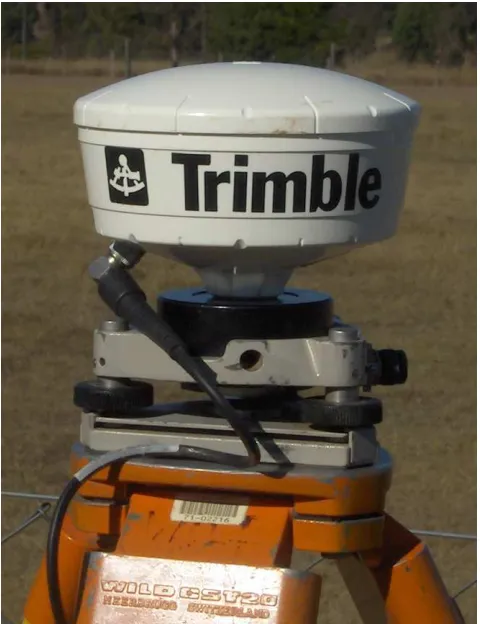
2.2.1 Pro XH Receiver

[image:20.595.114.370.492.763.2]

(21)

2.2.2 Pro XR Receiver

[image:21.595.113.353.287.599.2]

The Pro XR receiver is capable of real-time sub metre accuracy and is also fitted with EVEREST multipath rejection technology. The difference between the Pro XR and Pro XH receivers is that the Pro XR is unable to collect H-Star data or be post-processed using multiple base stations. Post-post-processed carrier phase accuracy for this receiver ranges from 30cm after 5 min of tracking satellites to 1 cm after 45 min of satellite tracking, this is the accuracy claim stated by Trimble. See Appendix C for Pro XR Specifications.

Figure 2.2: Photograph of Pro XR Receiver

2.2.3 Zephyr Antenna

(22)

features make this antenna ideal for data collection in areas where satellite signals may be degraded due to environmental conditions. A screw thread allows for easy mounting on a pole, tribrach or backpack. The zephyr antenna will be used with the Pro XH receiver. The reason this antenna is used instead of the internal antenna of the Pro XH, is the increased accuracy that the zephyr antenna can provide. This antenna cannot be used with the Pro XR receiver.

Figure2.3: Photograph of Zephyr Antenna

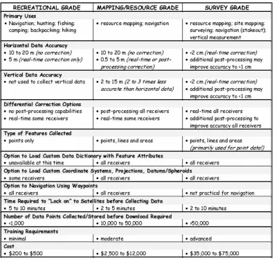
2.3 Grades of GPS Receivers

(23)

2.3.1 Survey Grade

Survey grade GPS receivers have the highest accuracy of the three grades, with typical accuracy of <2cm in real-time and after post-processing can reach <1cm. Typical survey grade receivers will have a purchase price of $35,000 to $70,000. The primary uses for receivers of this quality are resource mapping, surveying, stakeout and vertical measurement. These receivers undertake measurements by using carrier phase wave lengths.

2.3.2 Mapping/Resource Grade

Mapping grade receivers have reasonable accuracy of 0.5 to 5.0m for either real-time or post-processed corrections. $2,500 to $12,000 is the typical price range for receivers of this grade. The main use of this receiver type is, as its name suggests, for mapping resources which is used to provide spatial information for GIS.

2.3.3 Recreational Grade

Recreational grade receivers are used by hunters, fisherman and other outdoor activities where navigation is important. Typical receivers will cost up to $500 and have and accuracy of up to 5 m after a real-time correction has been made. These receivers are used predominantly to navigate safety back to a predetermined point such as a cabin or deer hide.

(24)

[image:24.595.116.512.56.431.2]

Figure 2.4: The comparisons between the three grades of GPS receivers (Source: Wisconsin Department of Natural Resources, 2001)

2.4 Past Testing Procedures

2.4.1 Testing by Trimble

(25)

of data collected. The increase in accuracy needs to be determined, so that is why testing is completed using external antennas. The use of the zephyr antenna with the Pro XH receiver can be used to see if there is any improvement in the accuracy by using an external antenna. This particular testing also involved static performance under canopy and dynamic performance under canopy. However, the testing of the receivers under canopy and dynamic performance is not important to this project, as the observations will be taken when the receiver is static over a particular mark.

Once the testing was concluded the Root Mean Square (RMS), and in particular Horizontal RMS (HRMS) value was calculated. The smaller the HRMS value the better the relative accuracy. RMS error is used to describe uncertainty and summarise the entire error distribution. The results of the testing undertaken by Trimble are shown in Figures 2.5 and 2.6.

Figure 2.5: Static accuracy by antenna configuration in open sky conditions (Source: Trimble 2006e)

Figure 2.6: Static accuracy and productivity by antenna configuration under canopy (Source: Trimble 2006e)

Note: This testing also compared productivity of the antenna configurations

(26)

the marks at the same time of day. By taking observations at the same time of day this ensured that the environmental conditions are very similar and will have the same effects on observations. This is one of the strategies employed by Trimble to ensure comparable data sets. The taking of observations at the same time every day is not going to provide the same range of environmental conditions that would be encountered when undertaking normal field. Field work is normally taken at different times of the day, as personnel and resources become available for use. That is why the testing undertaken by this project will visit the various Permanent Survey Marks (PSMs) at differing times that are more likely to be a representation the actual process involved in field work. This testing undertaken by Trimble has been helpful in explaining how a testing regime is conducted, but is of limited use because of the testing done under trees and the dynamic testing that was also completed.

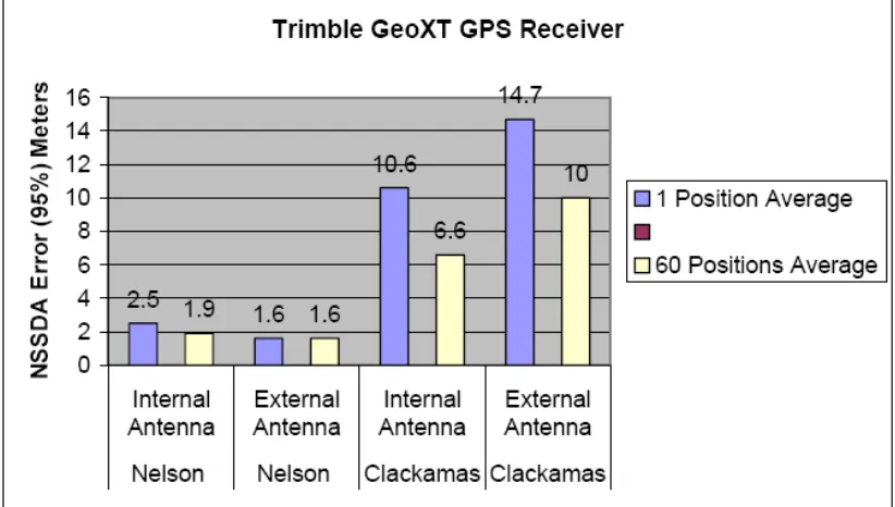
2.4.2 Testing by US Forest Service

Similar testing procedures were used by the US Forest Service to determine receiver performance under West Oregon forest canopies (Chamberlain 2002). Testing was carried out on 12 marks of known ordinates; once again these marks were co-ordinated using total station measurements. A lot of the existing testing regimes that have been found and examined have used conventional total station to co-ordinate the marks needed to test over. This will not be necessary for this project as the details of co-ordinated PSMs will be gained from the Department of Natural Resources and Water (DNRW) survey data base.

(27)

[image:27.595.116.527.82.315.2]

Figure 2.7: Results achieved from testing regime (Source: Chamberlain, 2002)

Nelson is an open site with no obstructions, while Clackamas is a forested site.

(28)

2.4.3 Testing by Serr, Weber and Windholz

Serr, Weber and Windholz (2006) undertook their testing regime to study which receivers would be the most appropriate for various research, remote sensing and GIS applications. It is important to know the practical accuracy of GPS receivers because their use in GIS applications is increasing. GPS data is being used to geo-reference satellite imagery and aerial photographs. New imagery systems such as Quick bird are able to achieve a spatial resolution of 2.4 m per pixel. To ensure that the geo-referencing is performed correctly the GPS receivers must be capable to deliver results that are one half of the spatial resolution of the imagery. This makes sure the each field observation is registered to the correct image pixel. The study was conducted in and around the city of Pocatella, Idaho. The receivers used in this testing regime were:

1. Trimble Geo XT with WAAS 2. Trimble Geo XT without WAAS 3. Trimble GeoExplorer II

4. Trimble Pro XR

5. HP IPaq with Pharos Navigation software and antenna.

Once again a number of pre-existing co-ordinated marks were chosen as the basis of the testing procedure. Serr, Weber and Windholz (2006) chose control marks based on their accessibility and visibility to GPS satellites. This is partly relevant to the testing completed as part of this project, as control marks have been selected based on their accessibility. This was done to provide the best conditions under which the receiver could operate. These conditions represent the environments that targets are placed in to geo-reference aerial photography and satellite imagery. Trimble Quick Plan software was used to plan the observation periods, when the Position Dilution of Precision (PDOP) was less than 5.0.

(29)

These testing procedures emphasise the following main points which are important to GIS database managers.

1. understand the differences in horizontal accuracy obtained from various GPS receivers

2. ensure co-registration of GPS acquired features and satellite or aerial imagery 3. determine the appropriate GPS receiver to use to satisfy mapping scale

requirements.

This testing procedure shows the need to undertake independent testing to ensure that the practical limitations of the receivers being used are suitable for the desired use. The original reason for this was to study which receivers would be the most appropriate for various research, remote sensing and GIS applications. The main reason why a variety of receivers are being tested as part of the testing regime for this project is because of the currently high use of mapping grade GPS receivers in the maintenance of spatial databases.

2.5 Post-processing GPS data

GPS measurements are effected by a number of different error sources. These errors affect the time for satellite signals to reach the receiver on the earths’ surface, and thus the computed position is inaccurate. Many of these errors are due to the limitations of the equipment and the environment in which the receiver is being used. The types of errors in GPS measurements are satellite errors, the atmosphere, multipath, receiver error and selective availability (Trimble 2006d). Selective Availability was turned off on 2nd May 2000 after the announcement from the White house a day earlier (Collins, Hofmann-Wellenhof & Lichtenegger 2001, p 17). Satellite and receiver errors are a result of errors within the clocks used to measure the time for the signals to reach the receiver. Even though satellite clocks are very accurate, there are still inaccuracies which lead to errors in position measurements (Trimble 2006d).

(30)

receiver. Since the distance calculation assumes a constant speed, the delay leads to a miscalculation of the distance (Trimble 2006d). Multipath occurs when satellite signals bounce off reflective surfaces before reaching the receiver. This delays the signals to the receiver, and also leads to a miscalculation of the distance. Many receivers now have sophisticated multipath rejection software such as EVEREST Multipath Rejection Technology, which allows these errors to be minimised. Carrier phase waves are right hand circularly polarised, but once reflected off surfaces becomes left hand circular polarised. The software is able to reject these reflected waves and only allow the right hand polarised waves to reach the receiver.

(31)

2.6 Statistical Concepts

Accuracy and precision are two terms that will be used throughout the discussion of the results achieved from the testing procedure; there is some confusion over the use of these terms since they are used interchangeably. Accuracy and precision do actually differ in their reference to measurements. Accuracy refers to the agreement between a measurement and the true or correct value (Bellevue Community College, 2005). The true or correct value needs to be known or able to be determined for accuracy of any measurements to be discussed and analysed. Accuracy refers only to the ‘closeness’ of a measured value and the expected value and makes no statement regarding the ability at which these results can be reproduced. Figure 2.8 is an example of accurate measurements.

Figure 2.8: An example of accuracy (Source: Flatirons Surveying, Inc)

Precision on the other hand refers to the ability of which measurements can be repeated. Successive measurements can be ‘far’ from the true value but still be close together indicating low accuracy but high precision. Figure 2.9 shows how precise observations are closely grouped together. When observations are both accurate and precise, their relationship to the true value (bull’s eye) is pictured in Figure 2.10

(32)

Figure 2.10: An example of accuracy and precision (Source: Flatirons Surveying, Inc)

Uncertainty is another term that will be used in the statistical analysis of the results gained from the post-processing. Uncertainty is the interval in which future measurements are expected to be contained. Uncertainty is quoted by a confidence interval, which states that a certain percentage of future measurements should be expected to lie within a set amount from the true value. A confidence interval is stated as plus/minus some value from a central value, usually the mean of the data being tested. For example if the confidence interval is stated as 0.5m ± 0.15m, means that it can be expected that results gained will be between 0.35 and 0.65m.

Confidence intervals are used to show what should be expected if repeated measurements are taken. A confidence interval is the range in which successive measurements are expected to be within, at a given percentage of confidence. An example of a confidence interval is represented in Figure 2.11.

Figure 2.11: An example of a confidence interval (Source: Flatirons Surveying, Inc)

(33)

2.7 H-Star Technology

H-Star post-processing is a method of post-processing GPS observations. H-Star technology is a combination of advanced GPS receiver, field software with sophisticated logging capabilities, and office software with innovative post-processing capabilities (Trimble 2006a). This method uses multiple base stations to differentially correct measurements taken by the receiver while out in the field. The three essentials for the H-Star system are:

1. Quality GPS data 2. PPA-driven workflow 3. H-Star post-processing

The GPS receivers used in H-Star processing are constructed to a high standard: therefore the equipment is able to capture a better quality of GPS signals. Since the GPS data collected is of a higher quality it is less likely to contain errors such as multipath to the same magnitude as receivers that don’t have H-Star capabilities.

(34)

is the PPA of all post-processed points collected during that time, when lock is regained the PPA will be recalculated as duration of lock increases.

Figure 2.12: The TerraSync software showing a PPA value (Source: Trimble 2006a)

To ensure that post-processed results are of the best possible quality, the reference stations used need to be of the highest quality. The quality of a reference station is shown as a value known as an integrity index. These values range from 0 to 100, the higher the value, the more reliable the reference station is for use in post-processing observations.

H-Star technology because of its PPA-driven workflow makes data capture more efficient; the reason for this is that the PPA indicates the accuracy that can be achieved once post-processing is complete. Without the use of H-Star, lock needs to be maintained for extended periods to ensure that post-processed results will meet designated specifications. The PPA value is continually calculated and displayed on screen and the operator is able to cease data collection once the required PPA value is reached, thus saving field time.

(35)

[image:35.595.113.507.55.317.2]

(36)

2.8 Conclusion

It can be seen that there are many similarities in the testing procedures examined. The main point is that a number of existing co-ordinated marks are chosen as references to determine accuracy of the receivers being tested. The number of points chosen is usually about twelve.

Another common factor is that testing is done while the receivers are static and set up over the mark for extended periods of time. The RMS values are always calculated and used as a basis for comparison against manufacturer claims and other receivers. A variety of receivers and antennas have been used by the individuals who are undertaking the testing observation regime. Data is post-processed from nearby base stations that are continually monitoring GPS satellites.

(37)

Chapter 3

Testing Procedures

3.1 Introduction

This chapter explains the testing regime, field and office procedures and stipulates why these procedures were appropriate to this project. The testing will be based on existing testing methods as reviewed in Chapter 2 and other specific procedures that will ensure that the project aim is met.

The aim of this chapter is to provide enough information to the reader to allow them to understand what the testing procedure involves, how this was completed and why this was done.

(38)

3.2 Data Characteristics and Testing Overview

To allow statistical analysis to be performed enough data needs to be collected for a period of time that can be considered to be a representation of the expected operating conditions. The data collected needs to be compatible with the software packages used for the processing of data. This should not be a problem as Trimble Pathfinder Office and Trimble Geomatics Office are designed to process the data files that the receivers will output. The output from the receivers is an un-corrected file in the .SSF file format.

The receivers that will be tested, namely the Trimble Pro XR and Pro XH, will be stationed at each mark and data will be logged at a rate of one position per second until the receiver indicates it has logged enough data for an adequate fix. Time taken for the receiver to record enough data for an adequate fix depends on many factors such as satellite geometry and environmental conditions surrounding the receiver whilst in use. The time taken for the Pro XR receiver to log enough data is indicted by a message shown on the screen of the data collection device, in this case a Recon. The message shown on the screen of the Recon was ten minutes. Ten minutes was therefore also used with the Pro XH receiver, even though this receiver is able to collect H-Star data and there is no such thing as minimum time required for an adequate fix.

(39)

Table 3.1: Manufacturer claims for the Pro XH

Post-processing Method Accuracy (HRMS)

with internal antenna 30cm

H-Star processed with optional zephyr

antenna 20cm

with 20 minutes of

satellite tracking 10cm

Carrier Post-processed

with 45 minutes of

satellite 1cm

Table 3.1 also shows the expected accuracy when using the zephyr antenna; this is why this project will test this antennas operation. It can be seen in Table 3.1 that as observation time increases so does the accuracy.

3.2 Observation and Post-processing Regime

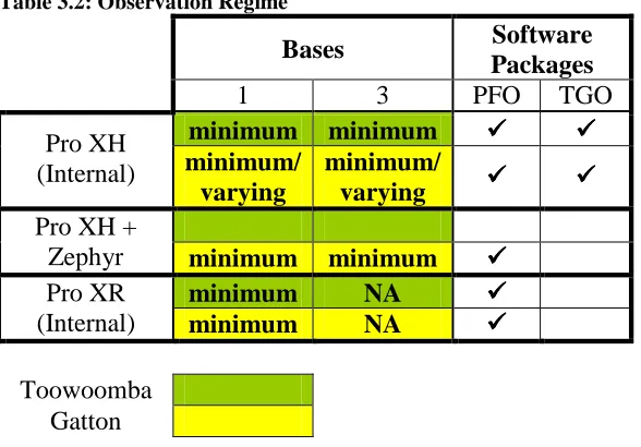
[image:39.595.114.408.510.715.2]

This section will explain the observations taken by each receiver configuration and which software programs will be used to post-process the data collected. The observation regime used for the project is shown in Table 3.2.

Table 3.2: Observation Regime

Bases Software

Packages

1 3 PFO TGO

minimum minimum

Pro XH

(Internal) minimum/ varying

minimum/

varying

Pro XH +

Zephyr minimum minimum

minimum NA

Pro XR

(Internal) minimum NA

Toowoomba Gatton

(40)

respective internal antennas and the zephyr antenna with the Pro XH. The minimum observation time was ten minutes, which is based on the time taken by the Pro XR to ‘collect’ enough data to calculate an adequate fix. This time was also used with the other two configurations. Two other times will also be used to test the receivers, which were twenty and forty-five minutes. The twenty minute observations were gained by deleting the last twenty-five minutes of a forty-five minute data file. These extended observation times will use the Pro XH receiver only and be carried at the marks surrounding Gatton. The exact testing carried with each receiver is shown in the following subsections

3.2.1 Pro XR Testing

H-Star post-processing will not be carried out with the Pro XR receiver as this receiver is unable to collect H-Star data. The Pro XR receiver will be used to take minimum time observations on all the marks (refer to Appendix D for list of PSMs used) and no extended observations will be carried out using this receiver. These observations will be post-processed using Path Finder Office. Single base station post-processing will be carried out using base station files from Ananga only.

3.2.2 Pro XH Testing

(41)

3.2.3 Pro XH and Zephyr Antenna Testing

The zephyr antenna will be used to compare the accuracy differences between the internal antenna of the Pro XH and the zephyr antenna. Observations taken with the zephyr antenna will only be of the minimum time of ten minutes and over the Gatton marks only. Observations taken with the zephyr antenna will be post-processed using Path Finder Office only.

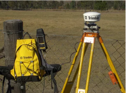
3.3 Field Procedures

[image:41.595.115.530.410.717.2]

The first step in the field procedure was the successful location and identification of the PSMs to be used during testing. This ensured that when testing was completed, the marks can be quickly and reliably located and the right mark used. Once individual marks had been located, the receivers were setup on a stable platform in this case a tripod.

(42)

The receiver remained on the tripod during the entire observation period. Observations were taken over a number of days as testing could not be completed in one day. The minimum time observations were completed first using the Pro XR receiver and the remaining observations were taken over subsequent days. Table 3.3 shows the date when each receiver configuration was tested.

Table 3.3: Observation Dates

Receiver/Marks Date

Pro XR/Toowoomba 7 July 2006

Pro XH/Toowoomba and Gatton 10 July 2006

Pro XH (extended)/Gatton 11 July 2006

Pro XR and Pro XH with Zephyr

Antenna 12 July 2006

Minimum time observations will test the ability of the onboard receiver software to determine when sufficient data has been logged, to ensure that the post-processed accuracy will be within manufacturers’ claims. Extended observations will determine whether there are any changes in accuracy as observation time increases. Results from this testing have been compared with claims made in the equipment specifications. The optimum observation time for efficient data collection can also be determined, but this is outside the scope of this project.

3.4 Office Procedures

Once the data had been collected in the field, it was post-processed using two different software packages: Trimble Pathfinder Office and Trimble Geomatics Offices (refer to Appendix F for Trimble Pathfinder Office post-processing settings and Appendix G for Trimble Geomatics Office project properties and processing style).

(43)

second, data from the base stations was also logged at this rate. This happens to be the standard logging rate at the base stations used to post-process the data collected.

Data from the minimal time observations was post-processed from Ananga, because of the ease of access to base station files. The varying baseline lengths have allowed changes in accuracy to be seen as the baseline length changes.

Data from the extended observations of the procedure were processed using the same procedure as the minimal time observations. Data from the 45 minute block have been processed after twenty and forty-five minutes, as according to the manufacturer’s specifications. A twenty minute data file was gained by removing the last twenty-five minutes of a forty-five minute file. This processing has allowed changes in accuracy to be seen and compared as the observation time increases. Since this data was logged with the Pro XH, the data was processed using both single and multiple bases. The processing for this part of the testing was undertaken using Trimble Pathfinder Office and Trimble Geomatics Offices.

Data collected with the Pro XR, and the Pro XH with zephyr antenna, was only post-processed using Pathfinder office. The data collected with the zephyr antenna was post-processed using both single and multiple bases.

3.5 Pro XR Receiver

3.5.1 Test/Data Collection

As mentioned earlier the Pro XR receiver was used to take ten minute observations on PSMs around both Toowoomba and Gatton. Observations were collected using a Recon Data collector, using the settings as outlined in Appendix E.

3.5.2 Post-processing

(44)

carrier post-processing only. H-Star post-processing could not be undertaken as this receiver is unable to collect H-Star data. The single base used for this post-processing was Ananga, the base that is located on the top of Z Block of the Toowoomba USQ campus.

3.5.3 Expected Analysis

After the observation files had been post-processed using Path Finder Office, the results of these files have been analysed with a number of Pro XH post-processed results. Comparing all the minimum time observations of both receivers has allowed the differences between single and H-star post-processing methods to be discussed. This can be achieved because the same control marks were observed for the same period of time by both receivers. This comparison will show which of the two methods is able to produce more consistent results. Dividing the marks into ‘close’ and ‘central’, has provided a way to see if there are any benefits in H-Star post-processing with the Pro XH receiver

Results from ‘close’ marks have been used to determine if there is extra weight placed on any one base station in the network of the H-Star base stations used when post-processing Pro XH observations. While results from ‘central’ marks have been used to compare the differences in accuracy with the Pro XR and H-Star post-processing using the Pro XH receiver

3.6 Pro XH Receiver

3.6.1 Test/Data Collection

(45)

settings used with this receiver are the same as those used with the Pro XR and are outlined in Appendix E.

3.6.2 Post-processing

The Pro XH receiver is able to collect H-Star data as described in section 2.7. Post-processing of Pro XH data files were therefore carried out using single and multiple base station processing. All data files taken using this receiver were post-processed using Ananga as the single base and the H-Star base station network as shown in section 2.7.

The minimum time observations using the internal were post-processed using both Trimble Path Finder Office and Trimble Geomatics Office. By using two software packages to correct the data files the differences between the two software packages can be analysed.

The extended observations were taken for forty-five minutes over ‘central’ PSMs only. These files were post-processed after twenty and forty-five minutes as set out in the manufacturer’s specifications as exhibited Appendix B. The twenty minute observations were obtained by removing the last twenty-five minutes of a forty-five minute data file. These data files were post-processed in Trimble Path Finder Office only.

The zephyr antenna data files were processed using single and multiple base stations. Observations for this configuration were restricted to the minimum observation time of ten minutes and taken over ‘central’ PSMs only. These files were only post-processed using Trimble Path Finder Office.

3.6.3 Expected Analysis

(46)

between increased observation times and increased accuracy. By using both single and multiple base station post-processing the differences can be seen between the two methods, this will be discussed further in chapter four.

The zephyr antenna results have been compared with the minimum time observations taken with the internal antenna. The manufacturers have claimed that the zephyr antenna is able to collect data of a higher quality than the internal antenna. Comparing these two different data sets has allowed the claims by the manufacturer to be tested.

3.6 Conclusion

By using the above mentioned observation and post-processing regime, the results can be analysed in a number of ways that will allow the different characteristics of the Pro XR and Pro XH receivers to be compared with each other. The main difference between the receivers is that the Pro XH data can be post-processed using multiple base stations, while the Pro XR cannot. The observation regime has been designed to see if there is any difference in using single base station post-processing when compared to multiple base post-processing. The way in which PSMs have been chosen for use in this project has allowed the opportunity to compare post-processed results as baseline length increases.

(47)

Chapter 4

Results

4.1 Introduction

This chapter shows a number of graphs of the results from each of the software packages, Trimble Pathfinder Office and Trimble Geomatics Office. The graphs will allow the reader to picture the differences between each of the post-processing methods and observation times used.

The aim is that the reader will gain an understanding of the differences between the results from each of the receivers with respect to the post-processing methods and observation times used by viewing the graphs in this chapter.

The graphs that have been constructed have been used in chapter 5: Analysis and Discussions. Each graph will be accompanied by a short paragraph explaining what is depicted on the graph above. The graphs have been divided into two sections, Trimble Pathfinder Office Pro XR and Pro XH and Trimble Geomatics Office Pro XH.

4.2 Explanation of results shown

(48)

distance error from the ‘true’ value was calculated by √ (∆E²+∆N²). The reduced level error was calculated as a difference from the ‘true’ reduced level value as published in the DNRW database for a particular PSM.

The software packages, Trimble Pathfinder Office and Trimble Geomatics Office were compared using HRMS and Vertical RMS (VRMS). RMS error is used to describe uncertainty and summarise the entire error distribution. The HRMS describes the error in the distance component. HRMS is calculated by finding the square root of the average of all the distance errors squared. VRMS describes the error in the reduced level component. VRMS is calculated by finding the square root of the average of all the reduced level errors squared.

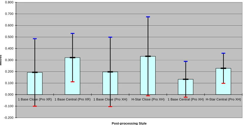
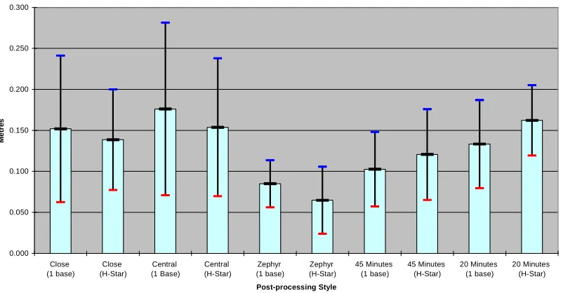
The graphs below show the 68% confidence intervals. The average is shown by the large horizontal bar in the middle, with the respective bounds shown by smaller bars at the top and bottom. The 68% confidence interval is the range between the upper and lower bounds as depicted by the blue and red bars respectively.

The graphs have been divided into their respective software packages; this has been done to give the reader some idea as to the individual results of each software package. The final section will show graphs that will be used to compare the two software packages against each other.

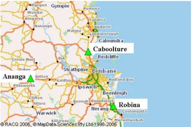
The graphs in this chapter refer to marks as ‘close’ and ‘central’. ‘Close’ is used to describe marks that are in close proximity to the base station Ananga as shown in Figure 2.13, ‘Central’, on the other hand, is used to describe the five marks located central to the H-Star base stations.

4.3 Analysis to be undertaken

(49)

After completing the post-processing of the observations that were taken according to sections 3.5.2 and 3.6.2, there were a number of comparisons that could used to check the various claims made by the manufacturers of the equipment tested. The comparisons used in this analysis were:

• one base & H-Star processing methods,

• how distance from base station affects post-processed results, and

• base station network weighting

The results have been compared using these three comparisons as a basis. These three comparison areas have provided the opportunity to see the difference between single and H-Star post-processing methods and see if H-Star is significantly better than single base station post-processing. The changes in accuracy as baseline length increases can be seen by using these three areas of comparison. The final area of analysis was to see if there is extra weight placed on any base in the H-Star base network. Extra weighting in the base station network would be proved by the fact that results from marks close to Ananga using single base station post-processing would be very similar to those obtained using H-star methods.

4.4 Trimble Pathfinder Office Pro XR and Pro XH

Comparison between 1 base and H-Star (Distance)

0.000 0.050 0.100 0.150 0.200 0.250 0.300

1 Base Close (Pro XR)

1 Base Central (Pro XR)

1 Base Close (Pro XH)

H-Star Close (Pro XH)

1 Base Central (Pro XH)

H-Star Central (Pro XH)

Post-processing style

M

e

tr

e

[image:49.595.124.522.514.723.2]

s

(50)

The difference between the Pro XR and Pro XH receivers is shown in Figure 4.1; the marks used in this figure have been divided into two categories ‘close’ and ‘central’ marks as described in section 4.2. The various post-processing methods used for each receiver are shown on this Figure. It can be seen that there is little difference between average distance errors of the two receivers when post-processing ‘close’ marks form a single base. There is quite a difference however in the confidence interval indicating that the Pro XH receiver is more reliable.

Comparison between 1 base and H-Star (Reduced Level)

-0.200 -0.100 0.000 0.100 0.200 0.300 0.400 0.500 0.600 0.700 0.800

1 Base Close (Pro XR) 1 Base Central (Pro XR) 1 Base Close (Pro XH) H-Star Close (Pro XH) 1 Base Central (Pro XH) H-Star Central (Pro XH)

Post-processing Style

M

e

tr

e

[image:50.595.122.525.250.455.2]

s

Figure 4.2: Comparison of 10 minute observations with respect to reduced level error

(51)

[image:51.595.124.525.83.292.2]

Average and standard deviation of all Pro XH observations (Distance) 0.000 0.050 0.100 0.150 0.200 0.250 0.300 Close (1 base) Close (H-Star) Central (1 Base) Central (H-Star) Zephyr (1 base) Zephyr (H-Star) 45 Minutes (1 base) 45 Minutes (H-Star) 20 Minutes (1 base) 20 Minutes (H-Star) Post-processing Style M e tr e s

Figure 4.3: Comparison of all observations taken by the Pro XH GPS receiver with respect to distance error

Figure 4.3 shows all observations taken by the Pro XH receiver. It can be seen that the zephyr antenna is able to collect satellite signals a lot better than the internal antenna of the Pro XH receiver. Also as observation time increases, so does accuracy. H-Star results for the twenty and forty-five minute observations were not as accurate as the single base station results. This difference may be the result of conditions at the Caboolture and Robina base stations not being representative of those at the testing sites.

Average and standard deviation of all Pro XH observations (Reduced Level)

[image:51.595.126.522.524.734.2]

-0.200 -0.100 0.000 0.100 0.200 0.300 0.400 0.500 0.600 0.700 0.800 Close (1 base) Close (H-Star) Central (1 Base) Central (H-Star) Zephyr (1 base) Zephyr (H-Star) 45 Minutes (1 base) 45 Minutes (H-Star) 20 Minutes (1 base) 20 Minutes (H-Star) Post-processing Style M e tr e s

(52)

Shown in Figure 4.4 are the average and confidence interval of the difference from the ‘true’ value in RLs for all observations taken by the Pro XH receiver. The observation times in this graph vary between ten, twenty and forty-five minutes. In some instances the results of H-Star post-processing were worse than post-processing from a single base, for example observations taken by the internal antenna of the Pro XH receiver were not as accurate as observations post-processed using a single base station.

Pro XR - Post-processed from Ananga

-0.600 -0.400 -0.200 0.000 0.200 0.400 0.600 0.800 1.000 1.200 PSM 40424 (1.04) PSM 40435 (1.84) PSM 112927 (5.36) PSM 40963 (5.80) PSM 59005 (6.35) PSM 112928 (6.67) PSM 40827 (8.39) PSM 61043 (9.38) PSM 35751 (10.42) PSM 107948 (32.94) PSM 1901 (35.38) PSM 132088 (36.42) PSM 89889 (36.47) PSM 61742 (38.04) PSM Names D if fe re n c e f ro m T ru e ( M e tr e s ) ∆E ∆N ∆RL Distance

[image:52.595.124.505.261.463.2]

Figure 4.5: Difference from the ‘true’ in Easting, Northing, Reduced Level and Distance from the ‘true’ as baseline increases from Ananga using the Pro XR receiver

(53)

4.5 Trimble Geomatics Office Pro XH

Comparison between 1 base and H-Star (Distance)

-0.500 0.000 0.500 1.000 1.500 2.000 2.500

Close (1 base) Close (H-Star) Central (1 base) Central (H-Star)

M

e

tr

e

s

[image:53.595.123.522.117.322.2]

Figure 4.6: Average and standard deviation for ten minute observations with respect to distance error

(54)

Comparison between 1 base and H-Star (Reduced Level)

-0.200 -0.100 0.000 0.100 0.200 0.300 0.400 0.500 0.600 0.700 0.800

Close (1 base) Close (H-Star) Central (1 base) Central (H-Star)

M

e

tr

e

s

Figure 4.7: Average and standard deviation for ten minute observations with respect to reduced level error.

(55)

Average and standard deviation of all Pro XH observations (Distance) -0.500 0.000 0.500 1.000 1.500 2.000 2.500 Close (1 base) Close (H-Star) Central (1 base) Central (H-Star) 45 Minutes (1 base) 45 Minutes (H-Star) 20 Minutes (1 base) 20 Minutes (H-Star) Post-processing Style M e tr e s

[image:55.595.123.523.82.285.2]

Figure 4.8: Comparison of all observations taken by the Pro XH GPS receiver with respect to distance error

Figure 4.8 shows how varying observation times and post-processing methods affect the average and standard deviations of distance errors. This graph clearly shows that the H-Star post-processing method did not perform as well as expected. The reason for this is that baselines from Caboolture and Robina were not fixed.

Average and standard deviation of all Pro XH observations (Reduced Level)

-0.200 -0.100 0.000 0.100 0.200 0.300 0.400 0.500 0.600 0.700 0.800 Close (1 base) Close (H-Star) Central (1 base) Central (H-Star) 45 Minutes (1 base) 45 Minutes (H-Star) 20 Minutes (1 base) 20 Minutes (H-Star) Post-processing Style M e tr e s

Figure 4.9: Comparison of all observation taken by the Pro XH GPS receiver with respect to reduced level error

[image:55.595.123.527.460.665.2]

(56)

[image:56.595.122.526.102.313.2]

Pro XH - Post-processed from Ananga -1.500 -1.000 -0.500 0.000 0.500 1.000 1.500 PSM 40424 (Fixed) PSM 40435 PSM 112927 (Fixed) PSM 40963 PSM 59005 (Fixed) PSM 112928 (Fixed) PSM 40827 PSM 61043 PSM 35751 (Fixed) PSM 107948 PSM 1901 (Fixed) PSM 132088 (Fixed) PSM 89889 (Fixed) PSM 61742 PSM Names D if fe re n c e f ro m T ru e ( M e tr e s ) ∆E ∆N ∆RL Distance

Figure 4. 10: Difference from the ‘true’ in Easting, Northing, Reduced Level and Distance from the ‘true’ as baseline increases from Ananga using the Pro XH receiver

(57)

4.6 Comparing Trimble Pathfinder Office and Trimble

Geomatics Office

RMS Values for post-processing in Path Finder Office

0.000 0.050 0.100 0.150 0.200 0.250 0.300 0.350 0.400 0.450

Pro XR (1 base)

Pro XH (1 base)

Pro XH (H-Star)

Zephyr (1 base)

Zephyr (H-Star)

45 Minutes (1 base)

45 Minutes (H-Star)

20 Minutes (1 base)

20 Minutes (H-Star)

M

e

tr

e

s

HRMS VRMS

Figure 4.11: Horizontal and Vertical Root Mean Square for observations post-processed in Trimble Pathfinder Office

[image:57.595.122.526.158.365.2]

(58)

RMS values for post-processing in Trimble Geomatics Office

0.000 0.200 0.400 0.600 0.800 1.000 1.200 1.400

Pro XH (1 base)

Pro XH (H-Star)

45 Minutes (1 base)

45 Minutes (H-Star)

20 Minutes (1 base)

20 Minutes (H-Star)

Post-processing Style

M

e

tr

e

s

HRMS VRMS

[image:58.595.125.524.81.294.2]

Figure 4.12: Horizontal and Vertical Root Mean Square for observations post-processed in Trimble Geomatics Office

(59)

4.7 Conclusion

The Figures shown in this chapter were been used in the discussions presented in the following chapter. The discussions that will be presented in chapter 5 have been based on section 4.3. The discussions in the next chapter will give a detailed explanation of what the Figures in this chapter represent. The next chapter will make continual references to Figures presented in this chapter.

(60)

Chapter 5

Analysis and Discussion

5.1 Introduction

This chapter links to the previous chapter in which the results were shown by a series of graphs. The discussions presented in this chapter are based on the areas identified in section 4.3. The main areas of analysis discussed in section 4.3, and presented in sections 3.5.2 and 3.6.2, were:

• single base compared against H-Star processing methods,

• how distance from base station affects post-processed results, and

• base station network weighting

The discussions in this chapter revolve around these key issues.

The aim of this chapter is to explain and interpret more thoroughly the results of the project to facilitate an understanding of the findings. The reader should understand the differences in accuracy between the Pro XR and Pro XH receivers and the use of the zephyr antenna with the Pro XH receiver after reading this chapter. Upon reading this chapter the accuracy differences between single and H-Star post-processing methods will be understood.

(61)

5.2 Post-processing with Pathfinder Office

5.2.1 One base and H-Star Processing Methods

5.2.1.1 Pro XR and Pro XH Internal Antennas

GPS data can be post-processed using a single base station or multiple base stations. The advantage of a multiple base station processing method is the ability to correct for atmospheric errors that surround the work site (refer to Figure 2.13). Results show that there is minimal difference between post-processing with one base or using multiple bases with H-Star processing if the marks are close to one physical base (refer to Figure 4.1). The average distance error from the true value was very similar for both post-processing methods (0.1382m for one base using the Pro XR and 0.1386m for H-Star using the Pro XH). This means if the marks are close to one of the physical base stations there is no real advantage in using H-Star post-processing.

It should be noted that the H-Star post-processing does however, produce smaller standard deviation values (0.1180 m for single base with the Pro XR and 0.0614 m for H-Star with the Pro XH). This means that even though both post-processing methods will achieve similar accuracies, the H-Star

Testing mapping grade GPS carrier phase accuracy