This is a repository copy of Geometric structure and geodesic in a solvable model of nonequilibrium process.
White Rose Research Online URL for this paper: http://eprints.whiterose.ac.uk/101404/
Version: Accepted Version
Article:
Kim, E. (2016) Geometric structure and geodesic in a solvable model of nonequilibrium process. Physical Review E - Statistical, Nonlinear, and Soft Matter Physics, 93 (6). 62127. ISSN 1539-3755
https://doi.org/10.1103/PhysRevE.93.062127
[email protected] https://eprints.whiterose.ac.uk/
Reuse
Unless indicated otherwise, fulltext items are protected by copyright with all rights reserved. The copyright exception in section 29 of the Copyright, Designs and Patents Act 1988 allows the making of a single copy solely for the purpose of non-commercial research or private study within the limits of fair dealing. The publisher or other rights-holder may allow further reproduction and re-use of this version - refer to the White Rose Research Online record for this item. Where records identify the publisher as the copyright holder, users can verify any specific terms of use on the publisher’s website.
Takedown
If you consider content in White Rose Research Online to be in breach of UK law, please notify us by
Geometric structure and geodesic in a solvable model of
non-equilibrium process
Eun-jin Kim1, UnJin Lee2, James Heseltine1, and Rainer Hollerbach3 1School of Mathematics and Statistics,
University of Sheffield, Sheffield, S3 7RH, UK
2Department of Ecology and Evolution,
University of Chicago, Chicago, IL 60637, USA and
3Department of Applied Mathematics,
University of Leeds, Leeds LS2 9JT, UK
Abstract
I. INTRODUCTION
A probabilistic description is essential for understanding the dynamics of stochastic
systems far from equilibrium, given uncertainty inherent in such systems. To compare
different Probability Density Functions (PDFs), it is extremely useful to quantify the diff
er-ence among different PDFs by assigning an appropriate metric to probability. This metric
structure then provides a key link between stochastic systems and geometry. Depending
on the question of interest, different metrics have been proposed (e.g. [1–10] and further
references therein). For instance, the Wasserstein metric has been studied extensively by
many authors in the optimal transport problem [9] in which the key problem is to minimize
transport cost, which is typically taken to increase quadratically with the distance between
two locations. For Gaussian measures, the Wasserstein metric is defined in the product
space consisting of Euclidean and positive symmetric matrices for the mean and variance,
respectively (e.g. see [4]). Compared with the Wasserstein metric, whose application has
established itself as a branch of applied mathematics, the geometric structure associated
with the information change in the Fisher (or Fisher-Rao) metric seems to be explored much
less. Unlike the Wasserstein distance, the Fisher metric provides a hyperbolic geometry in
the upper half plane (e.g [2, 7]) where the distance is measured in units ofthe width of the
PDF. That is, the distance in the Fisher metric is dimensionless and represents the
num-ber of different states in the statistical space. Such a notion was proposed in the seminal
work [11] where “statistical distance” was introduced as the number of indistinguishable
states between two PDFs. The purpose of our paper is to generalize this concept to
non-equilibrium systems and to quantify the rate of information flow by computing the change
in the number of indistinguishable states within these processes. This generalization will
endow non-equilibrium processes with geometric structure, providing a new perspective on
the link between stochastic processes and geometry.
The Fisher metric for Gaussian measures is related to the covariance, thereby also relating
to fluctuations in the systems. Specifically, [12] related the second moment of fluctuations
to the inverse of a metric tensor since strong correlations between any point and its
neigh-bors may emerge from large fluctuations, resulting in shorter distances around that point.
resolution (the unit of distance) set by the strength of fluctuations. Such fluctuation-based
metrics in thermodynamic states have been studied near equilibrium [11–14], for instance, in
the comparison of two equilibrium states via a statistical distance, or the interpretation of the
interaction in a system via the curvature of the metric tensor (e.g. near phase transitions).
A similar metric structure was also utilized in quantum systems [11, 15, 16]. Generalization
of this concept to non-equilibrium systems was attempted by different authors, although
they tend to be limited to the analysis of systems in near-equilibrium [14, 17–19]. Recent
efforts include the application of this concept to minimize entropy production within a
controlled system, or even the experimental measurement of statistical distance as a tool
to validate theory [14, 20–22]. As many systems in nature are not near equilibrium due
to intrinsic variability, heterogeneity, or uncertainty in a system [23, 34], our recent work
[23–25] focused on physical implications of the metric for the structure of an attractor and
the information flow in a strongly out of equilibrium system (e.g. music). In particular, [25]
presents a novel mapping between the non-equilibrium state and the distance to an attractor
by information length; [24] analyzed classical music by constructing time-dependent PDFs
from the music data stored in MIDI files.
The purpose of this paper is to investigate the information change associated with
non-equilibrium stochastic processes by using Fisher information metric and to provide a link
between geometric structure and a non-equilibrium process within a strongly out of
equilib-rium system using an exactly solvable model. We then examine implications of a geodesic
for which the information propagates at a constant speed. In particular, we show how our
results can be utilized in controlling a system. It is the aim of our work to inform the
potential utility of information length which can provide a powerful tool to unify different
non-equilibrium processes. The remainder of the paper is organized as follows. Section 2
provides an information interpretation of out-of-equilibrium processes. Section 3 introduces
our model (the generalized non-autonomous Ornstein–Uhlenbeck process) and provides some
important statistical relations. A general geodesic solution is presented in Section 4, and
specific solutions with prescribed boundary conditions are investigated in Section 5.
Sec-tion 6 expands on physical realizability of a geodesic soluSec-tion. An example of controlling a
system by utilising a geodesic motion is presented in Section 7. Conclusions are provided
as well as the derivation of fluctuating Hamiltonian in relation to information velocity and
an equation of motion in the curved metric space, the Christoffel and curvature tensors.
Some of the included derivations are quite basic and are similar to related analyses by other
researchers but are nevertheless included here to make this paper self-contained.
II. INFORMATION CHANGE AND FLOW
As noted in Section 1, the fluctuation-based Fisher metric provides the number of states
measured in units of the resolution, which is set by the strength of fluctuations. To elucidate
the meaning of the resolution, it is worth recalling that in equilibrium thermodynamics, the
fluctuation of random variables is determined by the properties of the heat bath, which
is assumed to be fixed with infinite capacity. For instance, for the Maxwell-Boltzmann
distribution, the probability distribution function (PDF) of the state energy E is given by
p(E) =βe−βE, (1)
where β = 1/kBT (kB is the Boltzmann constant, T the temperature of the heat bath) is
the inverse temperature. When E ∝x2 (where x is the velocity of a particle), fluctuations
in velocity x in the system are proportional to the thermal energy kBT of the heat bath,
which determines the variance (the width) of the PDF in Eq. (1), and consequently the
resolution on which the state E is differentiated. The finer the resolution, the more
dis-tinguishable different states are, and therefore the amount of accessible information in the
system increases. This can alternatively be interpreted that the thermal energy of the heat
bath provides a unit of energy for the probability, setting the unit of the information. This
is consistent with the view that the information increases with the increase in the gradient
of the PDF.
Many systems in nature are, however, far from equilibrium and there is no fixed
environ-ment that can serve as a heat bath for these systems [26]–[34]. In fact, one of the important
characteristics of these systems is that they are open and continuously interact with their
environment. The resolution of the PDFs and thus the unit of information evolve
dynam-ically at the same time as the PDFs change with time. It is thus important to model a
method is to use a stochastic forcing, for instance, via the following Langevin equation:
dx
dt =F(x) +ξ. (2)
Here, xis a random variable, and F is a deterministic force; ξ is a stochastic forcing, which
can for simplicity be taken as a short correlated random forcing as follows:
⟨ξ(t)ξ(t′)⟩= 2D(t)δ(t−t′). (3)
In Eq. (3), the angular brackets represent the average over ξ, ⟨ξ⟩ = 0, and D(t) is the
strength of the forcing, which can be prescribed as a function of time t. In this model,
the stochastic forcing ξ plays the role of heat reservoir in terms of the maintenance of the
fluctuations in the system, and in equilibrium the energy provided by the stochastic forcing
is balanced by the energy dissipation (the so-called fluctuation-dissipation theorem). This
model permits us to investigate the time evolution of a strongly out of equilibrium system
and the associated change in information.
As a system evolves out of equilibrium, the PDF of the state evolves in time, and
sub-sequent information change in the system is quantified by comparing the PDFs at different
times. In order to quantify the difference in PDFs which are changing with time, we use the
rate at which fluctuations change in time as the (time-dependent) resolution of the PDFs.
Specifically, the rate of change in PDFs defines the following information velocity v(t):
v2(t)=
!
dx 1 p(x, t)
"
∂p(x, t)
∂t #2
. (4)
The velocity v in Eq. (4) has units of inverse time, and quantifies the rate at which the
(dimensionless) information changes. As shown in Appendix A, the information velocity is
the RMS of the fluctuating Hamiltonian in a stochastic system, and τ = 1/v thus provides
a dynamic time unit as far as information is concerned. As shall be discussed shortly, a
geodesic is a special path which has a constant v where the metric is locally flat with no
net force acting on it. This is reminiscent of the constant speed of light as a photon travels
along a geodesic in curved spacetime.
time between the initial and final times t= 0 and t=tF in units of τ as:
L(tF) =
! tF
0
dt 1
τ(t) =
! tF
0
dt $
!
dx 1 p(x, t)
"
∂p(x, t)
∂t #2
. (5)
The accumulated change in information given by Eq. (5) provides the total change in the
information, and is the total distance between the initial and final PDFs in the statistical
space. We call L(t) in Eq. (5) the information length. The utility of a geodesic as an
optimal path which minimises the dissipated energy (or entropy production) has been
pre-viously invoked through the inequality relation between L and J as J(tF)tF ≥ (L(tF))2
where J(tF) =%t
F
0 dt[v(t)]
2= %tF
0 dt
% dx 1
p(x,t)
&
∂p(x,t) ∂t
'2
is the time integral ofv2. Note that
this inequality follows from the Cauchy-Schwartz inequality % v2dt%
u2dt≥(%
vudt)2 with
u = 1. The equality holds for the minimum path where v is constant (e.g. [22, 35]), and
the deviation from this equality quantifies the amount of disorder in an irreversible process
[35], or deviation from a geodesic. Given initial and final points in the parameter space, a
geodesic is an extreme path which minimises L; this is discussed in Section 3 in an exactly
solvable model.
A clearer geometric interpretation of the information velocity and length is possible when
control parametersλi (i= 1,2,3, ...) of a system are known, in which case Eqs. (4)–(5) can be expressed in terms of the metricgij based on the Fisher information (see, e.g. [14, 36, 37])
as follows:
v2(t) =E =
! dxdλ
i
dt gij dλj
dt , (6)
where
gij =
!
dx p(x, t)∂lnp(x, t)
∂λi
∂lnp(x, t)
∂λj . (7)
In Eq. (6), the velocity is defined in the control parameter spaceλi, where the metric tensor
gij in Eq. (7) gives the Riemannian metric [38]. For the Gaussian process that we will
consider later, λi represents the mean value and variance (see Eqs. (27) and (28)). That is,
the evolution of a non-equilibrium system can be viewed as the motion of a ‘particle’ with
unit mass travelling in the parameter space with the velocity v(t). Here the distance the
particle travels represents the information change. This dimensionless distance represents
the number of indistinguishable states that a system undergoes during the time evolution.
As shown in Appendix A, the information velocity is a measure of the RMS value of
of the relative entropy (or Kullback-Leibler divergence) (see Appendix in [25]).
Whilev2 is given either by Eq. (5) or Eq. (6), Eq. (5) has the advantage of enabling the
computation of information velocity and length directly from experimental/observational
data as long as the time-dependent PDFs can be constructed, even when control parameters
or governing equations of the system are not available. For instance, [24] has analyzed the
information flow and length in classical music by computing time-dependent PDFs from the
music MIDI files while [23] investigated an attractor structure in a logistic map by using
numerically computed time-dependent PDFs.
III. A SOLVABLE MODEL
The numerical computation of time-dependent PDFs is often extremely demanding. In
order to gain a key insight into the implication of information length and geodesics, it is thus
invaluable to utilize an exactly solvable model. To this end, we consider a linear,
driven-dissipative system for a stochastic variable x which damps due to a friction γ while driven
by an external stochastic forcing ξ as follows:
dx
dt =−γ(t)[x−f(t)] +ξ. (8)
Here, γ(t) is a non-negative friction constant; f(t) is a deterministic force which controls
the location of the equilibrium position. γ(t) orf(t) will be prescribed as a time-dependent
function for our purpose of finding a geodesic motion later. For simplicity, we take the
stochastic forcing ξ to have a short correlation time with the correlation function given in
Eq. (2) with the amplitudeD =D(t) which can depend on time in general. Whenf = 0 and
γ and D are constant, Eq. (8) is the Ornstein–Uhlenbeck process, which is a prototypical
model for a noisy relaxation system and has been utilized and extended in many areas of
physical science and financial mathematics (e.g. [39, 40]).
Given an initial condition x = x0 at t = 0, the solution to the stochastic differential
equation (8) is simply
x(t) =x0e−G(t)+
! t
0
where G(t) =%t
0 dt′γ(t′) andG(t1) =
%t1
0 dt′γ(t′).
For the assumed Gaussian process ξ, the transition probability between the position x0
at t= 0 and the final position xat time t is given by
P(x, t;x0,0) =
*
β1(t)
π exp[−β1(t)(x−y1(t))
2]. (10)
Letting the angular brackets denote the average overξ, we then have for y1(t) andβ1 as the
mean values of xand the inverse temperature, respectively:
y1(t) =⟨x⟩=x0e−G(t)+F(t), (11)
1 2β1(t)
=⟨[x(t)−y1(t)]2⟩=
! t
0
dt1e−2[G(t)−G(t1)]2D(t1), (12)
F(t) = ! t
0
dt1e−[G(t)−G(t1)]γ(t1)f(t1). (13)
To facilitate the analysis in the general case where the initial positionx0 is random with
the mean value µ, we assume the initial distribution of x0 to be the Gaussian distribution
with the inverse temperature β0
P(x0,0) =
*
β0
π exp[−β0(x0−µ)
2], (14)
which has a peak atx0 =µ. The PDF at a later time is obtained by integrating the product
of the transition probability (10) and the initial PDF (14) over x0 as:
P(x, t) = !
dx0P(x, t;x0,0)P(x0,0) =
*
β(t)
π exp[−β(t)(x−y(t))
2]. (15)
In Eq. (15), y(t) andβ(t) are the mean values averaged overx0 and ξ as:
y(t) =⟨⟨x⟩⟩= µe−G(t)+F(t), (16)
1
2β(t) =⟨⟨[x(t)−y(t)]
2
⟩⟩=⟨⟨(δx)2⟩⟩= e
−2G(t)
2β0 +
1
2β1. (17)
Here, β1 is given in Eq. (12); the double angular brackets ⟨⟨...⟩⟩ now denote the average
over both x0 and ξ; µ = ⟨⟨x0⟩⟩ and δx= x− ⟨⟨x⟩⟩. It is useful to note that β in Eq. (17)
satisfies the following relation:
β = β0β1
β1e−2G(t)+β0
= β0
e−2G(t)+q(t). (18)
q(t) = β0
β1
=−e−2G(t)+β0
β . (19)
For simplicity, the average over both ξ and the initial x0 will now be denoted by angular
A. Energy budget
In order to understand the role of D(t), f(t), andγ(t) in relation to information length,
it is useful to examine energy relations involving the second moment of x for macroscopic
energyy2 =⟨x⟩2 and fluctuating energy⟨(δx)2⟩, where δx= x−y. From Eq. (8), we obtain
by using the Stratonovich calculus [39–41]:
d dt
+ x2
2 ,
=−γ(t)x[x−f(t)] +ξx. (20)
The total workWξ by the external forcing between the initial time t= 0 and final time tis
obtained by the time integral of the last term in Eq. (20). This is computed by using Eqs.
(9) and (3):
⟨ξ(t)x(t)⟩=⟨ξ(t)δx(t)⟩= ! t
0
dt1e−[G(t)−G(t1)]⟨ξ(t)ξ(t1)⟩=D(t), (21)
Wξ =
! t
0
dt1⟨ξ(t1)x(t1)⟩=
! t
0
dt1D(t1). (22)
The average of the first term on the right-hand side of Eq. (20) gives us
⟨γ(x−f)x⟩=γy2+γ⟨(δx)2⟩ −γf y =γy(y−f) + γ
2β. (23)
Noting that the first and second terms on the right-hand side of Eq. (23) are due to the
mean and fluctuations, we can separate the time integral of the average of Eq. (20) as
1 2
(
y2−µ2) =
! t
0
dt1γ(t1)y(t1)[y(t1)−f(t1)], (24)
1 2
+1
β −
1
β0
,
=−Wγ +Wξ, (25)
where Wγ is the frictional energy loss from fluctuations to the environment:
Wγ =
! t
0
dt1
γ(t1)
2β(t1)
, (26)
and µ = y(t = 0) = ⟨x(t = 0)⟩ and β0 = β(t = 0). When β(t) = β0 at some time t, the
left-hand side of Eq. (25) vanishes, therefore Wξ = Wγ. That is, when the temperature is
equal at the initial and final times, the work Wξ is balanced by the total energy dissipation
Wγ. Alternatively, if Wξ and Wγ are not equal, then (Wξ −Wγ) and (β0 −β) having the
same sign implies that the temperature, and hence the PDF width, will increase or decrease
IV. GEODESIC MOTION
For the PDF in Eq. (15), a lengthy but straightforward algebra yields the information
velocity in Eq. (4) in the following form [25]:
v2 =E = 1 2β2β˙
2+ 2βy˙2, (27)
where ˙β= ddtβ and ˙y = dydt. By comparing Eq. (27) with Eq. (6), we can easily read off the metric tensor and control parameters as follows:
gij =
⎛
⎝
1 2β2 0
0 2β
⎞
⎠, λi =
⎛
⎝
β
y ⎞
⎠ . (28)
By using the Euler-Lagrange equations
dE
dβ −
d dt
dE
dβ˙ = 0, (29)
dE
dy − d dt
dE
dy˙ = 0, (30)
we obtain the coupled equations for the geodesic motion
¨
β− β˙
2
β −2β
2y˙2 = 0, (31)
d
dt[βy] = 0˙ . (32)
Here, Eq. (32) can be written as
βy˙ =c, (33)
where c is constant. When c = 0, the geodesic becomes y = constant and β ∝ lnt. By
using Eq. (33) in Eq. (31) and after some straightforward manipulation (see Appendix B),
we obtain
˙
β2 =−4c2β+αβ2, (34)
where α is another constant. To understand its physical meaning, we use Eq. (33) and Eq.
(34) in Eq. (31) to obtain:
v2 = 1 2β2β˙
2+ 2c2β= α
2. (35)
Thus, Eq. (35) implies that α is related to the information velocity as
v= *
α
A solution to Eq. (34) is found after some lengthy algebra (see Appendix B) as
β(t) = 2c
2
α
1
cosh√α(t−A) + 12 = 4c
2
α cosh
2
" 1 2
√
α(t−A)
#
, (37)
where A is constant. By using Eqs. (37) in (33), we then find the solution for y (see also
Appendix B):
y(t)=− √
α
c
1
1 +e√α(t−A) +B
= √
α
2c tanh "
1 2
√
α(t−A)
# −
√
α
2c +B, (38)
where B is another constant.
The identity sech2θ+ tanh2θ = 1 permits us to derive a useful relationship between β(t) and y(t) from Eqs. (37) and (38) as follows:
+
y+ √s
β∗ −B
,2 + 1
β =
1
β∗. (39)
Here
β∗ = 4c
2
α , s=
c
|c|, (40)
where s represents the sign of c. That is, if we think of y and √1
β being the variables, they
are related via a circle, with radius β1
∗ and centred at (0, B−
s
√
β∗). Geodesic motions are then along portions of this circle. This is a reflection of a hyperbolic geometry (the upper
half Poincar´e model) formed by y and the square-root of the temperature √1
β where the
centre of the circle Eq. (39) is at the boundary (i.e. on the axis where 1/√β = 0) of the
upper half plane. The location of the centre and the radius of the circle depend on the
particular problem of interest (see the next section).
To summarise, Eqs. (37)-(38) are general solutions for the geodesic, and the values of the
four constants c,α, A and B are to be fixed by the boundary conditions at the initial t= 0
and final timetF, depending on the problem of interest. A few specific examples are shown
in the following sections.
V. GEODESIC EXAMPLES AND SIGNIFICANCE
We now consider specific cases of the geodesic Eqs. (37)-(38) and examine the implications
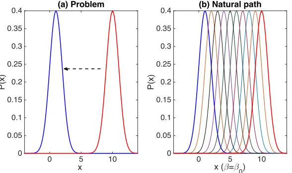
work required. As an illustration, we consider the time-evolution of a non-equilibrium state
shown in Fig. 1(a), where the mean position starts with the initial value y = y0 = µ
and approaches another non-equilibrium state y= yF which is closer to the equilibrium. As
boundary conditions, we consider the case where the initial and final temperatures are equal.
In terms of the PDFs, the width of the initial and final PDFs is thus the same, as shown
in Fig. 1(a), while the mean position of the PDF moves to the final point y = yF. The
key question of interest would be to find a path connecting the initial and final states which
minimizes the total information change, and to examine whether this path also minimizes
the time in addition to total energy dissipation. For instance, such minimization will be
particular useful when the initial state is very harmful, causing a lot of damage (e.g. a large
population of bacteria, etc., causing illness).
x
0 5 10
P(x)
0 0.05 0.1 0.15 0.2 0.25 0.3 0.35
0.4 (a) Problem
x (β=β0)
0 5 10
P(x)
0 0.05 0.1 0.15 0.2 0.25 0.3 0.35
0.4 (b) Natural path
FIG. 1: (a) A sketch illustrating the problem of moving a PDF from a larger (y0) to
smaller mean position (yF < y0), where the temperature (width) of the PDF is the same at
the initial and final timest= 0 andt= tF. (b) A natural path with the same temperature
β= β0 for all time between t= 0 and t=tF. The units of xare arbitrary.
A. Non-geodesic: β(t) =β0, γ(t) =γ0, and f= 0
As illustrated in Fig. 1(b), one possible and perhaps natural path connecting the initial
and final points would be to decrease the mean position while keeping the same temperature
[image:13.595.146.440.339.514.2]decreasingy exponentially in time through the constant frictional force asy =y0exp(−γt).
For a specific example, we consider the situation where y=y0 =µ at the initial timet= 0
and y= yF at the final timet=tF. Asβis the same at the initial and final times, Eq. (25)
gives a simple relation that the work done by ξ is dissipated by the frictional force, that is
Wγ = Wξ. These enable us to compute the total timetF and energy dissipation Wξ in Eq.
(22) simply as
tF =
1
γln
y0
yF
, (41)
Wξ =Wγ =
! tF
0
dtD =DtF =
1 2β0
ln y0 yF
. (42)
We can also compute the total information length using the result in [25] as follows:
L=32β0(y0−yF). (43)
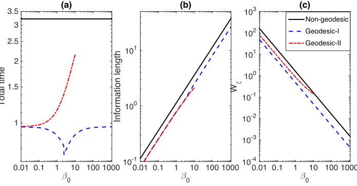
Solid black curves in Fig. 2 in panel (a), (b) and (c) respectively show the total time tF, L
and Wξ in Eqs. (41)–(43) againstβ0. These will be compared with results obtained for the
geodesic path.
β 0
0.01 0.1 1 10 100 1000
T
o
ta
l
ti
me
1 1.5 2 2.5 3
3.5 (a)
β 0
0.01 0.1 1 10 100 1000
In
fo
rma
ti
o
n
l
e
n
g
th
10-1 100 101
(b)
β 0
0.01 0.1 1 10 100 1000
W
ξ
10-4 10-3 10-2 10-1 100 101 102
103 (c)
Non-geodesic Geodesic-I Geodesic-II
FIG. 2: (a) Total time (b) Information length (c) Wξ against β0 in the non-geodesic case
(in solid black) and geodesic I (in dashed blue) and II (in dash-dotted red);
y(t= 0) =y0 = 5/6 and y(t=tF) =yF = 1/30. Geodesic II (dash-dotted red) is shown for
the value of β0 where the diffusion (DII) is non-negative. A distinct minimum in the total
[image:14.595.123.471.430.612.2]B. Geodesics
The natural path discussed above is not a geodesic as it does not satisfy Eq. (39). For a
circular geodesic motion, the change in y in time should be compensated by the change in
β. Specifically, since the initial and finalβ are equal,β should decrease in time initially and
then eventually increase back to the initial value β0 at the final time. That is, temperature
increases from 1/β0 to 1/β∗ > 1/β0 initially, and then at some point should decrease back to recover the value 1/β0 at the final time, and furthermore the system may need to go
through several cycles of periodic increase and decrease in temperature to satisfy a physical
realisability (e.g. see Fig. 5(d)).
It is useful to start with the simplest case of one cycle. To be specific, we take the total
time along the path to betF = 2A, and the values of the temperature andy at the midpoint
t = A to be β(t = A) =β∗ = 4c2/α < β
0 and y(t = A) = (y0+yF)/2 ≡yM, respectively.
Then, from Eqs. (37) and (38), we obtain
β(t) =β∗cosh2 "1
2 √
α(t−A)
#
, (44)
y(t) =−√1
β∗ tanh
" 1 2
√
α(t−A)
#
+yM, (45)
where we used c < 0 (as y0 > yF) and √α/2c = −1/
√
β∗. Therefore, the conditions
y(t= 0) =y0,y(t=tF) =yF,β(t= 0) =β(t=tF) =β0 give us the following relations:
y0−yF ≡∆=
2 √
β∗ tanh
"1
2 √
αA
#
, (46)
$
β0
β∗ = cosh
"1
2 √
αA
#
. (47)
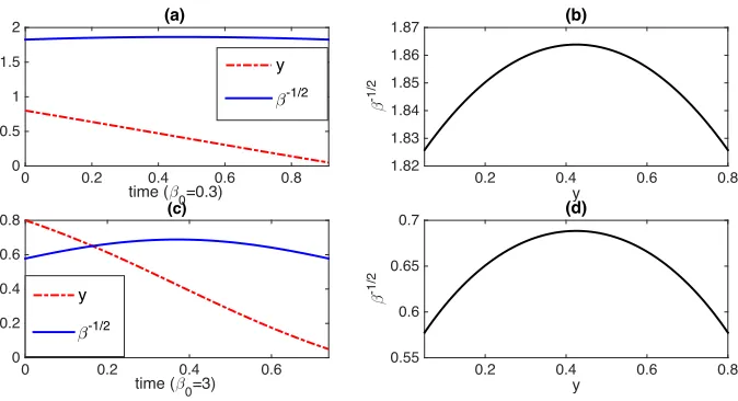
Typical behaviour of y and β−1/2 against time are shown in Fig. 3(a) and Fig. 3(c) for
β0 = 0.3 and 3, respectively, where we use y(t= 0) = y0 = 5/6 and y(t= tF) =yF = 1/30
and the value of α obtained in Section 4.B.1. Note that throughout the paper, we will use
these same value y0 = 5/6 andyF = 1/30 to facilitate comparison among different cases.
We recast Eq. (46) by using Eq. (47) to eliminate β∗:
∆= √2
β0 sinh
"1
2 √
αA
#
time (β0=0.3)
0 0.2 0.4 0.6 0.8
0 0.5 1 1.5 2 (a) y β-1/2 y
0.2 0.4 0.6 0.8
β -1 /2 1.82 1.83 1.84 1.85 1.86 1.87 (b)
time (β0=3)
0 0.2 0.4 0.6
0 0.2 0.4 0.6 0.8 (c) y β-1/2 y
0.2 0.4 0.6 0.8
[image:16.595.132.469.107.290.2]β -1 /2 0.55 0.6 0.65 0.7 (d)
FIG. 3: y and β−1/2 against time for β
0 = 0.3 and 3 in (a) and (c), respectively; the
corresponding geodesic circular segments in the (y,β−1/2) upper half-plane in (b) and (d),
respectively. In both cases, y0= 5/6 and yF = 1/30.
Eqs. (47)–(48) then give us
A= √2
αsinh
−1
"
∆√β0
2 #
= √2
αcosh
−1
$
β0
β∗, (49)
$
β0
β∗ = cosh
" sinh−1
"
∆√β0
2 ##
. (50)
In order to determine the total time 2Aand associated energy dissipation, we will shortly
find the value ofαand chooseγ(t),D(t) andf(t) in Eq. (8) to satisfy our derived equations
above. Before doing this through specific examples, it is useful to visualize the time-evolution
of general geodesic solutions. To this end, we note that β(t) andy(t) in Eqs. (44) and (45)
satisfy Eq. (39) where B−s/√β∗ is replaced by (y0+yF)/2 as
(y−yM)2+
1
β =
1
β∗, (51)
where yM = 12(y0 +yF). As Eq. (51) only depends on y0, yF, ∆ = y0−yF, β0 through
Eq. (50), Eq. (51) is independent of the information velocity (3α/2). Without specifying
the value of α, we can plot the geodesic motion from Eq. (51) in Figs. 3(b) and 3(d) by
using our fixed parameter values y(t = 0) = y0 = 5/6 and y(t = tF) = yF = 1/30 for the
two different values of β0 = 0.3 and 3, respectively. They clearly show the part of a circular
x (β
0=0.3)
-4 -2 0 2 4
PD
F
0 0.05 0.1 0.15 0.2 0.25 0.3
0.35 (a)
x (β
0=3)
-2 -1 0 1 2
PD
F
0 0.1 0.2 0.3 0.4 0.5 0.6 0.7 0.8 0.9
1 (b)
x (β0=30)
-2 -1 0 1 2
PD
F
0 0.5 1 1.5 2 2.5 3
3.5 (c)
x (β0=300)
-2 -1 0 1 2
PD
F
0 1 2 3 4 5 6 7 8 9
[image:17.595.121.471.120.432.2]10 (d)
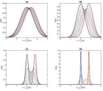
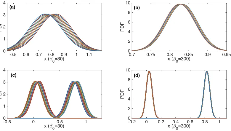
FIG. 4: Time evolution of PDFs against xfor β0 = 0.3,3,30 and 300 in (a)-(d), respectively. y0 =⟨x(t= 0)⟩= 5/6 and yF =⟨x(t=tF)⟩= 1/30. The initial and final
PDFs are shown by thick red lines on the right and blue lines on the left, respectively.
geodesic circular motion, it affects the speed at which a trajectory travels along it. That is,
the time scale on which y and β in Fig. 3(a) and 3(c) evolve depends on α (i.e. larger α,
faster evolution).
For completeness, the corresponding time evolution of the PDFs is shown in Fig. 4(a)
and Fig. 4(b) where the initial and final PDFs are plotted in red on the right and blue on
the left. The increase followed by decrease in the width of the PDFs (∝β−1/2) with time is
1. Geodesic I: Time varying D(t) and f(t)̸= 0with constant friction γ(t) =γ0
The total time tF = 2Adepends on the value ofα(orc), which is in turn determined by
the condition on f. Specifically, we require f(t= 0) = 0 att= 0 in the following.
Since ˙y =−γ0(y−f) andβy˙ =c, we recast f as
f =y+ 1
γ0y˙ =y+
c
γ0β. (52)
Thus, using f(t= 0) = 0 in Eq. (52) fixes the value ofc as
c=−γ0y0β0. (53)
By using Eq. (53) in Eq. (40), we obtain the value ofα as
√
α= 2γ√0β0y0
β∗ . (54)
Thus, from Eqs. (46), (49), (50), and (54), we obtain the total time tF = 2A for the
geodesic
2A= 2
γ0√β0y0
Q
coshQ, (55)
where
φ=3β0(y0−yF), Q= sinh−1
"
φ
2 #
. (56)
To compute the total work done by ξ, we observe that when γ(t) = γ0 is constant, G(t) =γ0t and G(t)−G(t1) =γ0(t−t1). By using them in Eqs. (12) and (17) and letting
D= DI(t) for Geodesic I, we obtain
2e2γ0tD
I(t) =
d dt
+ e2γ0t
2β
,
, (57)
and thus
2DI(t) =
γ0 β + 1 2 d dt + 1 β , = 1 β "
γ0−
√
α
2 tanh [ 1 2
√
α(t−A)]
#
. (58)
There is no contribution from the second term on the right-hand side of Eq. (58) toWξ for
our prescribed boundary condition β = β0 at t = 0 and tF; the contribution from the first
term is found by using β1 = 1cdydt (Eq. (33)) in Eq. (58):
Wξ =
! tF
0
dtDI(t) =
! 2A
0
dtγ0 2c
dy dt =
1 2β0
+ 1−yF
y0
,
time (β0=3)
0 0.2 0.4 0.6
0 0.2 0.4 0.6 0.8
1 (a)
y
β-1/2
y
0.2 0.4 0.6 0.8
β
-1
/2
0.55 0.6 0.65 0.7
0.75 (b)
time (β0=30)
0 0.2 0.4 0.6 0.8
0 0.2 0.4 0.6 0.8
1 (c)
y
0.2 0.4 0.6 0.8
β
-1
/2
0.182 0.183 0.184 0.185 0.186
[image:19.595.117.485.110.305.2]0.187 (d)
FIG. 5: y and β−1/2 against time in (a) and (c); The circular geodesics in the upper
half-planey and β−1/2 in (b) and (d) forβ
0= 3 and 30, respectively. In both cases,
y0= 5/6 andyF = 1/30.
While Eq. (59) is correct, a careful examination of the value ofDI(t) in Eq. (58) reveals
an interesting aspect about the information velocity 3α/2. That is, when α in Eq. (54) is
used in Eq. (58), DI can be shown to be negative for approximately the second half of the
time interval when the initial β0 is sufficiently large, specifically, when β0 > 3 for y0 = 5/6
and yF = 1/30 and for the fixed value γ0 = 1. The detailed discussion regarding the origin
of a negative DI is provided in Section 7. In order to satisfy a physically realistic condition
that DI is non-negative, we need to impose the constraint that the maximum value that
tanhθ [θ= √2α(t−A)] can take as
(tanhθ)max =
γ0
√
α/2 =
√
β∗ β0y0
. (60)
On the other hand, since Eq. (45) implies that the maximum value of tanhθ is√β∗(yM−
yF), we have
(tanhθ)max =
1 2
3
β∗∆, (61)
By equating Eqs. (60) and (61), we obtain the maximum value, say ∆m, of ∆ as
∆m=
2
β0y0
= 4σ
2 0
y0
, (62)
where σ0 = 1/√2β0 is the standard deviation of the initial/final PDF. ∆m is the largest
displacement in y that can be made before bringing the temperature back to the initial
value, and is referred to as the length of one cycle. The physical meaning of ∆m as the
maximum variation in y for a geodesic subject to the boundary conditions of the equal
temperature β = β0 at the initial and final time is provided in §7. When ∆m is smaller
than ∆=y0−yF, we will shortly show how to construct a geodesic solution which satisfies
boundary conditions. In a very special case where ∆m exactly matches ∆ – the so-called
resonance between two length scales – we obtain an interesting relation
∆= 2
β0y0
= 4σ
2 0
y0
. (63)
At this resonant point, tF takes the minimum value (see Fig. 2(a)), as discussed later.
We now present some detailed analysis on how to construct a geodesic solution when
∆m <∆. Leaving the most general analysis for future work, for the purpose of this paper
it suffices to consider a simple quantised case where there are an integer number of cycles of
length ∆m in ∆:
N = ∆
∆m
= ∆β0y0
2 , (64)
and divide the path between y0 and yF into N small cycles of length∆m. For example, the
geodesic for N = 10 is shown in Fig. 5(c)–(d) together with the case where N = 1 in Fig.
5(a)–(b) for comparison. Since all the cycles have the same time evolution of β while the
mean position of theith cycle changes as
y(Mi) = [(N−i) +1
2]∆m, (65)
where i= 1,2,3, ..., N, we can write down the geodesic equation for theith cycle by using
Eqs. (44), (45) and Eq. (65):
β(i)(t) =β∗cosh2 "
1 2
√
α(t(i)−A m)
#
, (66)
y(i)(t) =−√1
β∗tanh
"1
2 √
α(t(i)−Am)
#
where t(i)= [0,2A
m]; 2Am in Eqs. (66) and (67) is the time duration of theith cycle, which
can easily be found from Eq. (46) by replacing∆ by ∆m and by using Eq. (54) as
Am=
2√β∗ β0y0γ0
sinh−1
+
∆m
√
β0
2 ,
. (68)
Note that the time t in β(t) and y(t) in Eqs. (66) and (67) is the cumulative time over all
the cycles, computed as:
t=t(i)+ (i−1)(2Am), (69)
for i= 1,2,3, ..., N.
Fig. 5(c) shows the time history of β and y which undergo ten small-amplitude periodic
modulations; this modulation is more visible in Fig. 5(d). We note that the parameter
values in this figure were chosen to ensure an integer number of (specifically, ten) cycles.
By using these results, we now compute the total information length and total time by
adding the contributions from alli paths (i= 1,2,3, ..., N) as follows:
tF = 2AmN =
√
β∗∆ γ0
sinh−1
+ 1
√
β0y0
,
, (70)
L=tF
*
α
2 = √
2∆β0y0sinh−1
+ 1
√
β0y0
,
. (71)
To present results, we compute tF, L and Wξ by varying the value of β0 for y0 = 5/6 and
yF = 1/30, noting that for these values,∆= 0.8 and resonance∆=∆m occurs whenβ0= 3
for Geodesic I. Thus, when β0 < 3, N = 1 and we use results obtained for one cycle where
∆ = 0.8 (e.g. Eqs. (44)–(51)). When β0 > 3, we use the integer N number of cycles for
Geodesic I, by using Eqs. (70)–(71), and Eq. (59), together with Eqs. (64), (65), (66), (67),
(68) and (69). Results in Fig. 2 reveal a very interesting utility of Geodesic I. First, we
observe that Geodesic I results in much smaller values not only forLandWξ but also fortF,
compared with the non-geodesic case. Furthermore, a distinct minimum in the total time
is observed in Geodesic I around β0 = 3 due to the aforementioned resonance (∆m = ∆).
A corresponding time evolution of the PDFs for this resonant case is shown in Fig. 4(b).
This implies that for the given initial y0 and finalyF mean position, there exists an optimal
initial temperature (β0) which moves the PDF fromy0 toyF in the least time. These results
time (β 0=30)
0 0.2 0.4 0.6 0.8
-0.9 -0.8 -0.7 -0.6 -0.5 -0.4 -0.3 -0.2 -0.1 0
0.1 (a)
D
I(t)
f(t)
time (β 0=30)
0 0.05 0.1 0.15 0.2 0.25
0 5 10 15 20
25 (b)
D
II(t)
γ(t)
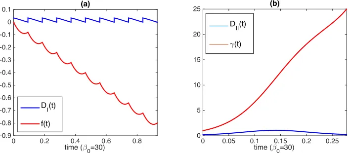
FIG. 6: (a) The blue upper curve shows DI(t), and the red lower curve shows f(t). (b)
The blue lower curve shows DII(t), and the red upper curve showsγ(t). For both panels
β0 = 30, y(t= 0) = y0= 0.08 and y(t=tF) =yF = 0.05.
total dissipated energy. Recalling that these results are obtained for a particular realization
of a geodesic consisting of a number of cycles with shorter length, further investigation into
other realizations would clearly also be worthwhile.
Finally, the time evolution of DI(t) and f(t) in Eqs. (58) and (52) are shown in Fig.
6(a) forβ0= 30, respectively. We see ten cycles (N = 10) of periodic modulation inDI and
f(t). The sign off remains negative, the significance of which will be discussed in a specific
problem in Section 6.
2. Geodesic II: Time varying friction γ=γ(t) and f(t) = 0
To determine the value ofγ(t) which is consistent with Eqs. (44) and (45), we utilise Eq.
(8) and βdydt =c in Eq. (33):
γ=−1
y dy
dt =− c
βy. (72)
Then, the use of the condition γ(t= 0) = γ0 in Eq. (72) gives us the value of c as
c=−γ0y0β0. (73)
By using Eq. (73) in Eq. (40), we obtain the value ofα as √
α= 2γ√0β0y0
[image:22.595.122.476.107.262.2]which is the same as Eq. (54). As in the case of Geodesic I in the previous subsection,
the diffusion D(t) can also become negative for sufficiently large β0. For the purpose of
formulating a theoretical framework in this paper, in the following, we limit our study to
one-cycle case for small β0 where DII is positive between t = 0 and tF. In this case, from
Eqs. (46), (49), (50), and (74), we obtain the total timetF = 2A for the geodesic
2A= 2
γ0√β0y0
Q
coshQ, (75)
where Q is defined as
φ=3β0(y0−yF), Q= sinh−1
"
φ
2 #
. (76)
The information length for the geodesic motion then simply follows from Eqs. (36), (74)
and (75) as:
L= ! 2A
0
dtv=√2αA. (77)
The computation of the total dissipated energy Wξ requires lengthier algebra. We refer
D as DII for Geodesic II and obtain from Eqs. (12) and (17) the following:
2e2G(t)DII(t) =
d dt
+e2G(t) 2β
,
, (78)
which essentially leads to the same equation (58) as,
2DII(t) =
γ β + 1 2 d dt + 1 β , = 1 β " γ− √ α
2 tanh [ 1 2
√
α(t−A)]
#
. (79)
We again note that there is no contribution from the second term on the right-hand side of
Eq. (79) to Wξ for the same β = β0 at t = 0 and tF, and the contribution from the first
term depends on γ(t). By using Eq. (72) in Eq. (79), we can rewrite Wξ as:
Wξ =
! tF
0
dtDII(t) =−
! tF
0
dt c
β2y. (80)
By using Eqs. (44), (45) and (73) in Eq. (80), and after further lengthy algebra (see
Appendix E), we obtain
Wξ =
1 2
" 1
β0 −y0yF
# ln y0
yF
+ 1 4 (
y20−yF2)
. (81)
Time evolution ofDII(t) andγ(t) for Geodesic II is shown in Fig. 6(b) forβ0 = 30, by using
the same values of y0 and yF as previously. We observe that the increase in the frictional
value (larger β) during the second half of the time evolution. Fig. 2 shows L, tF and Wξ
against β0, where they are seen to take small values compared to the non-geodesic case.
Information length for Geodesic I and II is observed to be small for sufficiently small β0. Note that in this figure, Geodesic II (in dash-dotted red) is shown for sufficiently small value
ofβ0 where the diffusion (DII) is non-negative. These results again point to the interesting
possibility of its application in optimisation.
VI. PHYSICAL REALIZABILITY OF A GEODESIC SOLUTION
In Section V.1, we noted that the diffusion coefficient can become negative as the initial
inverse temperature β0 becomes too large for fixed parameter values γ0,y0 and yF. In this
section, we expand on its physical meaning and realizability of a geodesic solution.
We begin by looking at the meaning of ∆m = 2/β0y0 = 4σ20/y0 in Eq. (62) in relation to
the information transfer by expressing the information velocity in Eq. (36) in terms of ∆m
as
v = *
α
2 =
γ0y0σ∗
σ2 0
= γ0(2σ∗) ∆m/2
. (82)
Here, σ0 =
3
1/2β0 is the standard deviation of the initial/final PDF and σ∗ =
3 1/2β∗
is the largest standard deviation (width) of the PDF when t = Am, where the inverse
temperature takes the smallest value β∗. Recall that the radius of the geodesic circle is
1/√β∗ =√2σ∗. Eq. (82) illustrates that the rate of information propagation across ∆m/2
is balanced by the frictional dissipation rate across the width of the PDF (2σ∗) at the
middle point. Alternatively, ∆m/2 is the largest distance over which the information can be
transferred physically for a given γ0.
In order to highlight the effect ofβ0 on cyclic solutions, it is useful to find an approximate
expression for σ∗ from Eq. (51) evaluated for the first cycle atβ =β0,y =y0 and ∆m/2 =
y0−yM:
+
∆m
2 ,2
+ 2σ02= 2σ∗2, (83)
which gives
σ∗ =σ0
" 1 + 2σ
2 0
y2 0
#12
where Eq. (62) was used. We define the change in σ0 and y0 for the first half cyclic motion
as
Dσ0 ≡σ∗−σ0, Dy0 =−∆2m =−
2σ2 0
y0
, (85)
and examine how they are related to each other in the two cases depending on the relative
ratio of the width σ0 of the initial PDF to y0.
In the first case where σ0 > y0/
√
2, Eq. (84) is approximated as
σ∗∼√2σ
2 0
y0 *
σ0, (86)
leading to Dσ0 ∼σ∗. Thus, Eqs. (85)–(86) give us
Dσ0
Dy0 ∼ −
1 √
2. (87)
Note that this limit supports a geodesic solution with N = 1. In the opposite limit of
σ0 < y0/
√
2, Eq. (84) is approximated as
σ∗ ∼σ0+
σ3 0
y2 0
, (88)
which leads to Dσ0 ∼ σ 3 0
y2 0
, and thus
Dσ0
Dy0 ∼ −
σ0
2y0
= Dy0
4σ0, (89)
where Eq. (85) is used (e.g. to eliminate y0 in place of Dy0). It is intriguing that Eqs.
(87) and (89) suggest very different scaling relations between Dσ0 and Dy0 depending on
whether the initial PDF has a width much narrower or wider thany0. Specifically, Eqs. (87)
gives a simple linear relation as
Dσ0
σ0 ∼ −
1 √ 2
Dy0
σ0
, (90)
where the normalisation of Dσ0 and Dy0 was made by the resolution σ0. In comparison,
Eq. (89) gives an interesting power-law relation, which can be expressed as follows:
4 4 4 4
Dy0
2σ0
4 4 4 4∼
+ Dσ0
σ0
,1/2
, (91)
where the normalisation by the resolution σ0 was again made. In comparison with Eq. (90), Eq. (91) implies a much smaller change in σ0 than y0 as a power-law. This is suggestive
Poincar´e half plane).
To examine the physical realizability of a geodesic solution, we rewrite Eqs. (91) and
(90) in terms of Dy0 =−∆m/2 as
|Dσ0|∝
⎧
⎪ ⎨
⎪ ⎩
∆m if σ0 * y0 ∆m
9
∆m
σ0
:
if σ0 + y0
, (92)
where ∆m/σ0 is factored out to highlight that for small σ0, |Dσ0|is larger than ∆m by this
factor∆m/σ0* 1. If∆m were to be the whole interval∆ =y0−yF,|Dσ0|∝∆2/σ0, which
becomes very large for small σ0. Although a geodesic solution is permitted for any value of
|Dσ0|, too large |Dσ0| can be problematic in its physical realisation in a particular model.
To see this, we recall that from §3, the change in the PDF width is due to the competition
between Wξ and Wγ. According to Eq. (92), when the total distance (∆ = y0−yF) that
the PDF needs to move is too large compared to the narrow width of the initial PDF,
the required change in σ becomes large; the PDF needs to become much wider than the
initial one along the geodesic (e.g. at the midpoint) and then become narrow to recover
β0. In order for the PDF to become narrower, the fluctuating energy (which is large for
a broad PDF at the middle point) needs to be removed by Wγ via frictional damping γ0,
which transfers the energy to the environment. For a fixed γ0 and y0 and yF, there is a
critical value of β0, above which the frictional damping is insufficient to accomplish this
task, causing a negative diffusion D. Alternatively, for the given initial β0 and y0, there is
upper bound ∆m on ∆ for a physically realisable geodesic solution.
VII. APPLICATION TO POPULATION GROWTH
A logistic-type equation is a popular model for population growth which has been widely
used to understand non-linear equilibration in many different systems. The merit of this
model is the simplicity in incorporating two conflicting effects of the positive feedback
(pro-moting the growth) and of the negative feedback (inhibiting the growth) via nonlinear
form [32]:
du
dt =γu−(-−ξ)u
2
−g(t)u2. (93)
Here u ≥ 0 is a non-negative random variable for the population; the terms involving
γ > 0 and - > 0 represent linear positive and nonlinear negative feedbacks, responsible
for the linear growth and the nonlinear saturation through competition, respectively. ξ
is the stochastic random part of the negative feedback which accounts for a stochastic
component of competition. For simplicity, ξ is assumed to be a short-memory noise given
by Eq. (3). The nonlinear term −g(t)u2 represents the reduction of the population by a prescribed deterministic force, which preferentially decreases larger populations, specifically,
as a quadratic power of u. Note that −-u2 represent the internal damping (negative
feed-back) mechanism while−g(t)u2 is damping by an external force which can be controlled for
a geodesic solution. Since time and u can always be normalised by γ and -, respectively,
we fix the value ofγ = 1 and-= 1 while varying other parameters for our study in this paper.
We envision the situation where we can control the time-dependence of the prescribed
x (β0=30)
0.5 0.6 0.7 0.8 0.9 1 1.1
PD
F
0 1 2 3 4
(a)
x (β0=300)
0.7 0.75 0.8 0.85 0.9 0.95
PD
F
0 2 4 6 8 10
(b)
x (β0=30)
-0.5 0 0.5 1
PD
F
0 1 2 3 4
(c)
x (β0=300)
-0.2 0 0.2 0.4 0.6 0.8 1
PD
F
0 2 4 6 8 10
[image:27.595.120.510.441.662.2](d)
FIG. 7: Time evolution of PDFs ofxover the first cycle forβ0= 30 and 300 in (a) and (b), respectively. (c)-(d) are the evolution of PDFs over the first and the last cycles (10th and
u (β 0=30)
5.4 5.6 5.8 6 6.2 6.4
PD
F
0 0.02 0.04 0.06 0.08 0.1
(a)
u (β 0=300)
5.7 5.8 5.9 6 6.1 6.2
PD
F
0 0.05 0.1 0.15 0.2 0.25 0.3
(b)
u (β 0=30)
0 1 2 3 4 5 6
PD
F
0 0.5 1 1.5 2 2.5 3
(c)
u (β 0=300)
0 1 2 3 4 5 6
PD
F
0 2 4 6 8 10
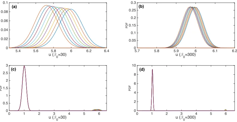
[image:28.595.118.515.119.324.2](d)
FIG. 8: Time evolution of PDFs of the population ufor β0 = 30 and 300, corresponding
to Fig. 7. ⟨u(t= 0)⟩= 6 ⟨u(t=tF)⟩= 1.0345, which is close to the carrying capacity
u∞ = 1 (γ = 1, -= 1). (a)-(b) show the PDF during the first cycle as in Fig. 7 (a)-(b),
where the PDF at t= 0 can be identified with the peak atu= 6. (c)-(d) are the evolution
of PDFs over the first and the last cycles (10th and 100th cycle for (c) and (d),
respectively) shown at the same time.
forcingg(t) and the strength of the stochastic noise ξ between the initial and the final states
and are interested in finding a best treatment protocol which reduces the population size
in the least time. This could potentially be very beneficial when a fast reduction of the
population (e.g. treatment of disease) is desired. This optimal protocol is provided by a
geodesic found in §5.
In order to utilise the results obtained in previous sections, we transform the nonlinear
equation Eq. (93) into the form of Eq. (8) by using the change of variable x=−1/u+-/γ
as follows:
dx dt =−γ
+ x+ g
γ
,
+ξ. (94)
By comparing with Eqs. (8) and (94), we identify thatf is replaced by−g(t)/γ. Therefore,
very conveniently, if we assume that x = −1/u+-/γ has the initial Gaussian distribution
time (β0=30)
0 0.2 0.4 0.6 0.8
0 0.1 0.2 0.3 0.4 0.5 0.6 0.7 0.8
0.9 (a)
D I(t)
g(t)
time (β0=30)
0 0.2 0.4 0.6 0.8
0 1 2 3 4 5 6
7 (b)
y
u
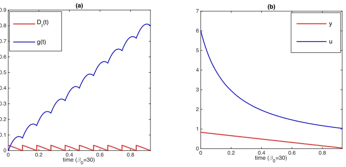
FIG. 9: (a) The red lower curve shows DI(t), and the blue upper curve shows g(t). (b)
The red lower curve shows y (the mean value of x), and the blue upper curve shows u. For
both panels β0 = 30, the carrying capacity γ/-=u∞ = 1,y(t= 0) =y0 =⟨x(t= 0)⟩= 5/6
and y(t=tF) =yF =⟨x(t=tF)⟩= 5/6.
yF at the initial and final times t = 0 and tF, respectively, the inverse temperature β(t)
and the mean position y(t) satisfy the same equations as in Eqs. (64)–(68). We recall that
the mean value denoted by the angular brackets is obtained by the average over both ξ
and initial position x0. Furthermore, by considering the situation where the objective is
to reduce the average population by keeping the same inverse temperature β = β0 at the
initial and final times and the constant growth rateγ =γ0, we can find the best treatment protocol which minimises the time and the associated dissipated energy by using a geodesic
solution (Geodesic I) forN cycle. We consider β0= 30 and β0 = 300 for the fixed values of y0 = 5/6 and y = 1/30, as in previous section. Therefore, N = 10 and 100 for β0 = 30 and
300, respectively. (Modest values of β0 are used for this model to ensure a negligible escape rate of the population to +∞.) The optimal treatment schedule g(t) is obtained from the
geodesic solution via Eq. (52):
g(t) =−γ0f(t) =−γ0
+ y+ c
γ0β
,
. (95)
Results are shown in Figs. 7–9 for the case where the carrying capacity u∞ = 1 and
y0 = ⟨x(t = 0)⟩ = 5/6 and yF = ⟨x(t = tF)⟩ = 1/30, the same values used in all other
[image:29.595.128.481.112.283.2]a geodesic consists of 10 (N = 10) and 100 (N = 100) cycles, respectively. Specifically,
the time evolution of PDFs of x over the first cycle for β0 = 30 and 300 are shown in Fig.
7 (a) and (b), respectively while the evolution of PDFs over the first and the last cycles
(10th and 100th cycle for β0 = 30 and 300) are shown in Fig. 7 (c) and (d), respectively.
Corresponding time evolution of PDFs of the population u is shown in Fig. 8. We note
that the PDF of u at t = 0 has a peak at ⟨u(t = 0)⟩ = 6, corresponding to y0 = 5/6;
⟨u(t=tF)⟩= 1.0345, which is close to the carrying capacity u∞= 1 (γ= 1,-= 1). Finally,
Fig. 9 shows DI(t), g(t), mean values of x and u against time for β0 = 30, where the sign
of g(t) is seen to be positive. Interestingly, the observation that the total change in g(t) is
comparable to ∆ = y0 −yF in Fig. 9 reveals how the geodesic solution is established by
slowly moving the PDF peak by the deterministic force.
VIII. CONCLUSION
Far from equilibrium, the level of fluctuations in a system changes with time and becomes
a dynamical variable itself, and the importance of a full knowledge of the evolution of PDFs
cannot be over-emphasized. As the computation of time-dependent PDFs is highly
de-manding and expensive numerically, we utilized one analytically solvable model of a driven
dissipative system (a generalized non-autonomous Ornstein–Uhlenbeck process) by
includ-ing the time-dependent deterministic forcinclud-ing and time-dependent strength of the stochastic
noise (diffusion). By generalizing our familiar concept of distance by using a dynamical
ruler whose resolution is set by time-dependent fluctuations, we mapped the time-evolution
of our system onto the trajectory in the statistical metric space given by the Poinc´are upper
half-plane consisting of the mean position and the standard deviation 1/√β. We computed
the information velocity and length and found geodesic solutions for which the information
propagates at constant speed to be either in the form of a line of a constant mean position
or a circle. We then demonstrated how to construct a particular realization of a geodesic
which satisfies boundary conditions at the initial and final times in the two specific cases of
Geodesic I and II and showed that in both cases, our realization of a geodesic provided a
path that ensures not only small information length and dissipated energy but also smaller
phe-nomenon in the geodesic solution due to the matching of∆ =∆m was reported for the first
time. Application of our results to a stochastic logistic model demonstrated a significant
improvement in controlling population growth by a periodic modulation of diffusion coeffi
-cient and deterministic force by a small amount. This optimization can have a significant
implication for damage control where the prolongation of a system near an initial condition
(e.g. a large population of harmful bacteria, a strong tornado, etc) is harmful.
Although we utilized an exact solution in this paper, our methodology is general and
does not rely on the existence of exact PDFs nor even the existence of basic equations which
govern the evolution of systems. This is because the information velocity and length can
be computed directly from Eqs. (4) and (5) by constructing time-dependent PDFs from
experimental/observational/numerical data. For instance, [23] numerically computed PDFs
by simulating a logistic map and the information velocity and length for the purpose of
investigating the attractor structure (e.g. stable/unstable points); [24] studied the
infor-mation velocity and length in classical music by computing time-dependent PDFs from the
music MIDI files, elucidating different classical music in terms of the information flow and
the role of geodesics in classical music. Application of our methodology to other data (e.g.
heart rhythm) is under progress. A geodesic solution can also be implemented numerically,
for instance, as has been done in [10]. In addition to this very applicability to a variety of
systems whose evolution is far too complex to be modelled by a system of equations, our
methodology will provide a unifying framework for understanding seemingly different
phe-nomena by using system-independent variables (information velocity and length, geodesics).
In summary, this paper provides a key theoretical framework for understanding
non-equilibrium processes in terms of information change and a new scope for investigation and
application of a geodesic to different non-equilibrium systems, particularly for the purpose
of optimization. Given our discovery of a novel resonance phenomenon, further investigation
into different realizations of a geodesic solution would be of great interest. Detailed analysis
on different realisations and different situations with appropriate boundary conditions will
be addressed in future papers. Further application and extension of this work to different
Appendix A: Fluctuating Hamiltonian E
To appreciate the relation between information velocity or energyE and fluctuating
en-ergy, we express the PDF p(x, t) as
p(x, t) = *
β
πe
−SA
≡e−SA+F. (A1)
Here, F = 12lnβπ is the free energy; SA is the effective action which can be related to the
Hamiltonian H of the stochastic system (see [42]) as
H =−∂SA
∂t , (A2)
which is a stochastic analogy to the Hamilton-Jacobi relation [42, 43]. Specifically, it was
shown in [42] by a path integral formulation that H is given in terms of
H(t) =−∂SA
∂t =
D 2Π
2−µΠx
where Π is the conjugate momentum. Note thatΠ stems from the stochastic noise. Taking
the time derivative of Eq. (A1) gives us
∂p(x, t)
∂t = ( ˙F+H)p(x, t), (A3)
where ˙F = dF
dt. First, we integrate both sides of Eq. (A3) over xand use the conservation
of the total probability as follows:
0 = !
dx∂p
∂t =
!
dx( ˙F+H)p(x, t) = ˙F+⟨H⟩, (A4)
where ⟨H⟩is the mean (average) value of the Hamiltonian. Therefore,
˙
F =−⟨H⟩. (A5)
That is, the mean value of the Hamiltonian compensates for the change in free energy to
conserve the total probability. We now compute the second moment which is related to E
in Eq. (6) as
E = !
dx1 p
+
∂p
∂t ,2
= !
dx(H+ ˙F)2p(x, t)
=⟨(H+ ˙F)2⟩=⟨(δH)2⟩, (A6) where δH = H − ⟨H⟩ = H + ˙F is the fluctuating Hamiltonian. By using Eq. (A5), it is
interesting to observe that
Appendix B: Derivation of Eqs. (34), (37) and (38)
By using Eq. (33) in (31), we obtain
¨
β− 1
ββ˙
2= 2c2, (B1)
which can be written as
β2 ∂
∂β
; ˙
β2 β2
<
= 4c2. (B2)
Dividing Eq. (B2) by β2 and integrating over β gives us
˙
β2
β2 =−
4c2
β +α, (B3)
where α is an integration constant. The rearrangement of Eq. (B2) gives Eq. (34) in the
text.
From Eq. (34), we obtain
dβ
dt = √
α
*
β2−4c2
α β, (B4)
which can be integrated as
√
α
! dt=
! dβ
=
β2− 4c2 α β
, (B5)
to obtain
√
αt=A+ cosh−1
+
αβ
2c2 −1
,
, (B6)
where A is constant.
Solving Eq. (B6) for β gives us Eq. (37) in the text.
To find the solution fory, we solve Eq. (33) for y by using Eq. (33) as follows:
1 cy(t)=
! dt1
β =
α
2c2
! t
0
dt coshθ+ 1
= α c2
! 2eθdt
(eθ+ 1)2
=− √
α
c2
1
eθ+ 1 +B, (B7)
Appendix C: The Christoffel and Ricci-curvature tensors
This appendix is included for completeness of our paper. From Eq. (27), the metric
tensor gij and its inversegij can be found as:
gij =
⎛
⎝
1 2β2 0
0 2β
⎞
⎠, gij =
⎛
⎝
2β2 0
0 2
2β
⎞
⎠ . (C1)
Connection tensorΓijk = 12[∂igjk+∂jgik−∂kgij] (Γijk =gimΓjkm) can be found to have the
following non-zero components
Γ111 =−
1
β,Γ
1
22 =−2β2,Γ212 =Γ221 =
1
2β. (C2)
The Riemann curvature tensor Ri
kmn = ∂mΓink +ΓimpΓpnk −∂nΓimk −ΓinpΓpmk can then be
shown to have the following non-vanishing components:
R1212 =−R1221 = −β, R2112 =−R2121 = 1
4β2. (C3)
As the curvature tensors do not vanish for certain components, the metric space is not
flat but curved. The Ricci tensor is then computed by contracting the curvature tensor as
Rij = Rkikj:
R11 =−
1
4β2, R22 =−β, R12 =R21 = 0, (C4)
leading to the Ricci scalar
R= gijRij = −1 (C5)
We now make an analogy to the Einstein field equation where Gij = 8πTij (whereTij is the
stress-energy tensor). By using R=−1 forGij
Gij =Rij−
1
2R gij = ⎛
⎝
−4β12 0
0 −β
⎞
⎠+
1 2
⎛
⎝
1 2β2 0
0 2β
⎞
⎠= 0. (C6)
Therefore, the stress-energy tensor Tij = 0.
Appendix D: Geodesic equation
It is worth noting that the Euler-Lagrange equations (29)-(30) can also be derived from
the following geodesic motion for E in Eq. (27) by using the Christoffel tensors in Eq. (C3):
d2λi
dt2 +Γ i mk
dλm
dt dλk
where λi = (β, y). Specifically, Eq. (D1) becomes
0 = ¨β+Γ111β˙2+Γ122y˙2, (D2) 0 = ¨y+Γ212β˙y˙+Γ221β˙y.˙ (D3) Using Eq. (C2) in Eqs. (D2)-(D3) gives us Eqs. (31)-(33).
Appendix E: Derivation of Eq. (81).
By using Eqs. (44), (45) and (73) in Eq. (80) and by letting θ = 1 2
√
α(t−A), we can
derive
2β∗Wξ =
!
dθ 1
cosh4θ(b−tanhθ) =−
!
dθ[ln (b−tanhθ)]sech2θ
= "
−ln (b−tanhθ) cosh2θ
#θF
θ0
−2J
≡I(t= 2A)−I(t=A). (E1)
Here, b =√β∗yM and yM = 12(y0+yF); θ0 and θF are the values of θ at t = 0 and t= 2A,
respectively;I(t= 0) andI(t= 2A) are the value of integral evaluated att= 0 and t= 2A,
respectively. J is defined as follows:
J = !
dθln (b−tanhθ) tanhθsech2θ
= − !
dw(lnw)(b−w)
= "
−b[wlnw−w] +1 2w
2lnw
−14w2 #wF
w0
= "
−12(b2−tanh2θ) ln (b−tanhθ) + 1
4(b−tanhθ)(3b+ tanhθ) #θF
θ0
, (E2)
wherew = (b−tanhθ) was used; w0and wF are evaluated att = 0 andt= 2A, respectively.
In order to compute Wξ in Eq. (E1), we need to evaluate the various terms at t = 0 and
t= 2A. For t= 0, we can show that
b−tanhθ=y0
3
β∗, b+ tanhθ=yF
3
β∗,
3b+ tanhθ= (2yF +y0)
3
β∗, cosh2θ= β0
β∗,
b2−tanh2θ =y0yFβ∗,