This is a repository copy of Bayesian Parameter Estimation and Model Selection of a
Nonlinear Dynamical System using Reversible Jump Markov Chain Monte Carlo
.
White Rose Research Online URL for this paper:
http://eprints.whiterose.ac.uk/81827/
Proceedings Paper:
Tiboaca, D., Green, P.L., Barthorpe, R.J. et al. (1 more author) (2014) Bayesian Parameter
Estimation and Model Selection of a Nonlinear Dynamical System using Reversible Jump
Markov Chain Monte Carlo. In: Proceedings of ISMA 2014, International Conference on
Noise and Vibration Engineering. ISMA 2014, International Conference on Noise and
Vibration Engineering, 15-17 September 2014, Leuven, Belgium. .
[email protected] https://eprints.whiterose.ac.uk/ Reuse
Unless indicated otherwise, fulltext items are protected by copyright with all rights reserved. The copyright exception in section 29 of the Copyright, Designs and Patents Act 1988 allows the making of a single copy solely for the purpose of non-commercial research or private study within the limits of fair dealing. The publisher or other rights-holder may allow further reproduction and re-use of this version - refer to the White Rose Research Online record for this item. Where records identify the publisher as the copyright holder, users can verify any specific terms of use on the publisher’s website.
Takedown
If you consider content in White Rose Research Online to be in breach of UK law, please notify us by
Bayesian Parameter Estimation and Model Selection
of a Nonlinear Dynamical System using
Reversible Jump Markov Chain Monte Carlo
D. Tiboaca, P.L. Green, R.J. Barthorpe , K. Worden
Dynamics Research Group, The University of Sheffield, Department of Mechanical Engineering, Sir Frederick Mappin Building, Mappin Street, S1 3JD, Sheffield, United Kingdom
e-mail: [email protected]
Abstract
The aim of this paper is to demonstrate the potential of the Reversible Jump Markov Chain Monte Carlo (RJMCMC) algorithm when applied to system identification problems which involve both parameter estima-tion and model selecestima-tion. Within the context of Bayesian Inference, Markov Chain Monte Carlo (MCMC) methods have been used for a long period of time to address the parameter estimation of linear and nonlinear systems, which are described approximately by a model. It is often the case that there are a set of competing model structures that could potentially produce good approximations of the real system - this raises the issue of model selection. Even though they address parameter estimation, many MCMC samplers cannot address model selection. As an extension to one of the most well known MCMC samplers, the Metropolis-Hastings algorithm, the RJMCMC algorithm is a MCMC method that covers model selection as well as parameter estimation simultaneously. RJMCMC can be applied when models contain different numbers of parameters. The algorithm is capable of moving between parameter spaces of different dimension in order to find the most appropriate model that describes the system and the most probable parameters within that model. In this contribution the RJMCMC algorithm is introduced in the context of nonlinear dynamical systems and is demonstrated on simulated data.
1
Introduction
System Identification has, for a long time, been an area of great importance in the context of structural dy-namics. The aim of system identification is to provide a robust characterisation of a real structure, making use of experimental data and mathematical models. The purpose of characterising the real structure is to assess its dynamic behaviour. As is well known, the process of system identification breaks down into two main areas: estimation of parameters that cannot be directly measured experimentally (parameter estimation) and identification of the mathematical model structure (model selection). From an industrial perspective, pos-sessing knowledge of the dynamic behaviour of a real structure is helpful as it can determine such things as the excitation a structure can withstand before damage or failure occurs or the maximum displacement a structure can withstand, etc.
Whatever the cause of nonlinearity, due to its unpredictable behaviour,a nonlinear structure can become problematic [6]. Nonlinearity is increasingly being considered as part of the reason why structures fail. For this reason, researchers are working on developing tools to deal with nonlinearity.
An important issue that one encounters when conducting system identification is that of uncertainty. Uncer-tainty could arise from either unknown, ignored or/and compressed information [8]. UncerUncer-tainty occurs for various reasons, such as measurement error, model selection error or parameter estimation errors, etc [3]. Whatever the provenance, uncertainty can affect the results of system identification, sometimes invalidating them [7]. One way of accounting for uncertainty in the process of system identification is by using a prob-abilistic framework. There are two main views when using a probprob-abilistic framework [10]: the Frequentist view or the Bayesian view. As the name implies, the frequentist approach is based on the frequency of out-comes; it does not take into account anything that happened before the event of study. Another probabilistic approach is Bayesian inference, which is the approach used in the present work. Bayesian inference is based on degrees of belief, which means that when constructing the probability of an event happening, one takes into account any prior information about that event. One of the benefits of using a Bayesian framework is that it prevents overfitting in the process of model selection. Due to the fact that Bayesian inference, often enough, makes use of posterior probability distributions with complex geometries, MCMC sampling algo-rithms are being used (MCMC algoalgo-rithms have the capacity of sampling from complex distributions). Over the years, there have been many MCMC sampling algorithms developed, but the Metropolis-Hastings(MH) algorithm which is presented in this current work, remains one of the most popularly used. The MH sam-pling method is used in doing parameter estimation but unfortunately it does not cover the process of model selection. Due to this shortcoming, the RJMCMC algorithm is introduced, which can simultaneously cover parameter estimation and model selection of nonlinear dynamical systems. The reason for the RJMCMC algorithm’s capacity of doing nonlinear system identification fully is due to its added benefit of being able to move between spaces of varying dimensions. Further explanations on the RJMCMC algorithm are provided in Section 4.
1.1 Literature Review
Some of the relevant work done in structural dynamics within the context of system identification using Bayesian inference and MCMC sampling methods is summarised next.
MCMC sampling methods have been widely used in research areas other than structural dynamics. Their wide application makes them even more attractive to researchers. Until 1990, MCMC algorithms were employed mainly in the areas of chemistry and physics. After 1990, the algorithms were introduced into statistics which provided an opportunity for them to be used in other research areas such as signal process-ing, structural dynamics, etc. [1].
reliability and possible ways of overcoming it. The algorithm introduced in [21] offered good results in SI when used on two models.
MCMC sampling algorithm within a Bayesian framework have been used for SI of nonlinear systems in the past. One example of such work by the current authors is [18]. The authors discussed the use of the MH algorithm on two models, a ’Bouc-Wen’ hysteresis model and a nonlinear model of Duffing type. The algorithm was used for the issue of parameter estimation and the Deviance Information Criterion in order to conduct model selection. This can prove time consuming and computationally expensive. A discussion on the correlation of the parameters was conducted.
Another example of using MCMC sampling methods and Bayesian inference for nonlinear system identifi-cation is [17]. The authors of this particular work used real data in order to conduct SI on nonlinear systems with nonlinearities of friction and stiffness.
The present work is mainly concerned with the RJMCMC algorithm which was introduced in 1995 by Green in [16]. The author introduced the RJMCMC algorithm as an extension to the MH algorithm with the added benefit of being able to do parameter estimation and model selection at the same time. In order to do so, Green proved that the Markov chain created by his algorithm obeys the principle of detailed balance while jumping between different parameter spaces. Another work by the same author [13], explains the RJMCMC algorithm in further detail.
Having [16] as a starting point, many researchers adapted the RJMCMC algorithm. An example of such work is [15] where the authors chose to use the Gibbs sampler rather than the MH algorithm at the core of the RJMCMC algorithm (the method was used on logistic and simulated regression problems).
The RJMCMC algorithm found its use on NARMAX(Nonlinear Autoregressive Moving Average with eX-ogenous input models) models as well [14]. The authors of [14] used the algorithm in order to present a comparison between the forward regression method and the RJMCMC, with the latter having several bene-fits.
Nuclear physicists have taken the opportunity to employ the RJMCMC algorithm as an alternative to linear and nonlinear least squares techniques [5]. The interest of the authors of [5] was to use MCMC methods in order to quantify the isotopic content of radioactive material. The methods proved successful in nuclear spectroscopy but the authors brought to attention the fact that when it comes to MCMC algorithms, the pro-cessing time can become an issue.
The paper is structured as follows. Section 2 will be an introduction to Bayesian inference and its relevance within system identification of dynamical systems. Section 2 also introduces the background of MCMC sampling methods and their importance in conducting Bayesian inference, concentrating on the Metropolis-Hastings sampler. Section 3 is concerned with briefly describing the RJMCMC method and how it was applied in the present work. Section 4 presents the results of applying the RJMCMC algorithm in nonlinear system identification, and Section 5 provides a conclusion and discussion to the present work.
2
Bayesian Inference and MCMC sampling methods
P(θ|D, M) = P(D|θ, M)P(θ|M)
P(D|M) (1)
and
P(M|D) = P(D|M)P(M)
P(D) (2)
whereθis the vector of parameters,Dis the available data,M is the selected model andM is the vector of
possible models.
As mentioned in Section 1, the existence of uncertainty might lead one to a probabilistic approach. The authors of the present paper used a probabilistic framework based on Bayesian inference due to the fact that a Bayesian framework prevents overfitting in the process of model selection (it follows Occam’s razor [10]) and also due to the fact that it makes use of prior knowledge (as limits for the parameters, information on material properties, etc.).
Equation (1) represents Bayes’ theorem used in the parameter estimation process and it states that the pos-terior probability distribution of the parameters is equal to the likelihood of the available data multiplied by the prior probability distribution of the parameters and divided by the evidence term.
Equation (2) represents Bayes’ theorem used in the model selection process and it states that the posterior probability distribution of the models is equal to the likelihood of the used data multiplied by the prior probability distribution of the models and divided by a normalising constant.
The evidence term of equation (1) is hard to evaluate analytically (complex integrals), which contributes to the fact that the posterior probability distribution has often enough a complex form.
In 1953, the physicists from Los Alamos, New Mexico, started using successfully the MCMC sampling methods, while working on the atomic bomb [20]. One algorithm of particular importance to the work of statisticians during WWII was the Metropolis algorithm, developed by N. Metropolis. Later on, around 1970s, statisticians made the discovery that Bayesian inference can make use of MCMC sampling methods in order to generate posterior probability distributions with complex forms, as these MCMC algorithms are capable of sampling from PDFs with complicated geometries (the generalisation of the Metropolis algorithm made by Hastings, which made available the widely used MH algorithm) [1].
In the context of structural dynamics (precisely SI), the Metropolis-Hastings algorithm together with Bayesian inference is popularly used today to address the process of parameter estimation. Briefly put, the MH algo-rithm works by generating samples from a target PDF,π(θ)(withθbeing the vector of unknown parameters),
using a proposal PDF,Q(θ′|θ), in order to provide samples from the posterior distribution of the parameters.
The popularity of the MH algorithm is due to the fact that the evidence term can be ignored in the sampling process and also due to the fact that the proposal PDF can have any form the user chooses. Convergence to the posterior distribution is guaranteed. For further details into how the MH algorithm is used in the context of parameter estimation of dynamical systems, the reader is referred to a previous work by the authors, [4]. In his paper [16], Green made an observation about the MH algorithm. When confronted with the issue of model selection, the Markov chain loses detailed balance as it is incapable of moving between spaces of varying dimensions. The author introduced the RJMCMC algorithm as an alternative to other meth-ods of conducting model selection as the RJMCMC algorithm proved to be capable of doing parame-ter estimation and model selection simultaneously, while obeying the principle of detailed balance as re-quired in order for the Markov chain to be able to provide samples. This happens when one has a set of models M = {M(1), M(2), ..., M(l), ..., M(L)} each depending on its own set of vector of parameters,
{θ(1),θ(2), ...,θ(L)}.
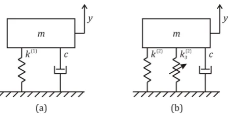
Fig. 1: (a) Linear system, (b) Nonlinear system of Duffing type
3
RJMCMC
The RJMCMC algorithm was first introduced in the well known paper [16]. This current work proposes to introduce the algorithm in the context of system identification of dynamical systems by applying it on two models, a SDOF linear model (M(1)) and a SDOF nonlinear model with a cubic stiffness (M(2)) as illustrated in Fig. 1.
For the first model, M(1), the mass m, damping coefficient c and data (comprised of y (output) which is displacement andF (input) which is the forcing), are assumed to be known or measured. The unknown parameter for estimation is the linear stiffnessk(1). ModelM(1)is mathematically described by equation (3).
my¨+cy˙+k(1)y=F (3)
For the second model,M(2), as for modelM(1),the massm, damping coefficient cand data are assumed to be known or measured which leaves the linear stiffness k(2) and the cubic stiffnessk(2)3 for estimation. ModelM(2)is described through equation (4).
my¨+cy˙+k(2)y+k(2)3 y3 =F (4)
In order to apply the algorithm, for the current contribution, the authors used simulated data from the linear and nonlinear models of the SDOF system. The main idea is to use the RJMCMC algorithm to do both model selection and parameter estimation for the simulated system. The RJMCMC algorithm comprises three types of moves:
• Birth move - attempt moving from modelM(1)to modelM(2)probabilistically;
• Death move - attempt moving from modelM(2)to modelM(1)probabilistically;
• Update move - stay in current model and update parameters using the MH algorithm(for details on how to apply the MH algorithm please refer to [4]);
The RJMCMC algorithm is explained below [12] [4]:
The quantitiesαm,α′m, are the acceptance probabilities of the birth and death moves respectively and will
[image:6.595.188.413.81.194.2]Algorithm 1RJMCMC Algorithm
forn= 1 :N do
2: Get umf rom U[0,1]−generates a random number f rom an unif orm distribution; ifum ≤b(
n)
l −birth move condition; then
4: −propose birth move
Generate ubf rom U[0,1]−generates a random number f rom an unif orm distribution;
6: Evaluate αm (detailed below) ifub ≤αm then
8: −update to model l+ 1and update model parameters;
else
10: −stay in model l;
end if
12: else
ifum ≤(b( n)
l +d
(n)
l )−death move condition;then
14: −propose death move
Get udf rom U[0,1]−generates a random number f rom an unif orm distribution;
16: Evaluate α′
m (detailed below) ifud ≤α′m then
18: −go to model l−1and update model parameters;
else
20: −stay in model l;
end if
22: else
normal M H algorithm, model remains at l state, update parameters only;
24: end if
end if
As explained in the RJMCMC algorithm, the birth move is attempted with probabilityblwhich is given by
equation (5). If the condition for the birth move is met, then the algorithm jumps from modelM(1)to model
M(2),
bl=pmin
1,P(l+ 1) P(l)
(5)
where, in this case,l= 1(which refers to modelM(1)) andl+ 1 = 2(which refers to modelM(2)). In the case of the birth condition not being met, the algorithm attempts a death move randomly by using equation (6). If the condition for a death move is met, then the algorithm will move from modelM(2) to modelM(1).
dl=pmin
1,P(l−1) P(l)
(6)
where, in this case,l= 2(which refers to modelM(2)) andl−1 = 1(which refers to modelM(1)).
If neither conditions for doing a birth or death move are met, then the algorithm will do an update move. As
bl,dlandulare probabilities, the update move is attempted randomly using equation (7).
ul= 1−(bl+dl) (7)
Referring to equation (5), (6) and (7), the constantpis used in order to adjust the update probability,ul, with
respect to the birth and death probabilities,blanddl. TheP(l)andP(l−1)components refer to the prior
probabilities of modelslandl−1, which according to the case, could be for modelsM(2)orM(1).
To recap, at this point there are two models:M(1)which represents a SDOF linear system that contains one unknown parameter - the linear stiffnessk(1)andM(2)which represents a SDOF nonlinear system that con-tains two unknown parameters - the linear stiffnessk(2)and the cubic stiffnessk3(2). In his paper [16], Green introduced the concept of dimension matching in order for the principle of detailed balance to hold while jumping between spaces of varying dimension. Detailed balance, within the RJMCMC algorithm, allows the Markov chain to provide samples from the mass probabilities of models while generating samples from the target probability of parameters.
Section 3.1. provides further explanations on the concepts of dimension matching and detailed balance.
3.1 RJMCMC and the Principle of Detailed Balance
As modelM(1)has only one unknown parameter and model M(2) contains two unknown parameters, one can easily spot a mismatch in dimensions. Due to the fact that the dimensions do not match, jumping from one model to the other in order to do model selection proves impossible when using the MH algorithm. What one wants to do is be able to move between the two models in order to decide which of them best fits the available data. In order for the forward and backward moves to occur, the principle of detailed balance needs to be respected (at equilibrium each process should be balanced out by its reverse process). As the dimensions of the two vectors of parameters for each of the two models do not match, the process of jumping fromM(1)toM(2)cannot be balanced out by its reverse process, i.e. jumping fromM(2)toM(1). An approach to solving the problem of matching dimensions is by introducing a new parameter in model
relate different states [9]). In order to move fromM(1) toM(2), the following mapping,h:R2 →R2, was introduced:
( k(2) k(2)3
) = 0 µ + k(1) λ (8)
whereµis a chosen value that needs to be tuned in order for the algorithm to reach a solution efficiently. The inverse of the mapping is applied for a death move, i.e. for going fromM(2)toM(1).
The form of the mapping is not chosen randomly. Green also mentioned in his paper [16] that in order for the mapping to be used in jumping between spaces it needs to be diffeomorphic. A diffeomorphic mapping means one that is differentiable and unique. It is obvious that the created mapping is differentiable. One is left with proving that the mapping is unique. According to the inverse function theorem, as long as the Jacobian at whichever chosen point is nonzero, the mapping is said to be unique [9]. Furthermore, in this particular case, the determinant of the Jacobian is calculated to be unity under all conditions. This concludes the mapping to be differentiable and unique, i.e. diffeomorphic.
Now, having introduced a new parameter inM(1) and having proven the chosen mapping to be diffeomor-phic, one can endeavour to prove that the detailed balance principle holds with the RJMCMC algorithm. From this point onwards, expressions of the formπ(θ) are considered to be probability density functions
(PDFs).
In the context of SI of dynamical systems, the principle of detailed balance states that:
π(θ)T(θ→θ′)dθ=π(θ′)T(θ′ →θ)dθ′ (9)
Equation (9) can be explained as: the taget PDF,π(θ), of the vector of parameters θ, multiplied by the
transition functionT(θ → θ′)between the vector of parametersθand the new stateθ′, has to be equal to
the taget PDF,π(θ′), of the vector of parametersθ′, multiplied by the transition functionT(θ′ →θ)between
the new state of the vector of parametersθ′and the current state of parameters vectorθ.
The transition function mentioned in equation (9) can also be written in the following form:
T(θ→θ′) =q(θ′|θ)α(θ→θ′) (10)
whereq(θ′|θ′) is the proposal density used in the sampling process. Considering that equation (9) is valid
for all paths available between the vector of parameters:
Z
π(θ)T(θ→θ′) dθ=
Z
π(θ′)T(θ′→θ) dθ′ (11)
Writing equation (10) for the case where there are two unknown parameters:
Z Z
π(θ)q(θ′|θ)α(θ→θ′) dθ
1dθ2 = Z Z
π(θ′)q(θ|θ′)α(θ′ →θ) dθ′
1dθ2′ (12)
If one considers equation (12) in the case of the two modelsM(1)andM(2), one has model(1)depending on a vector of parametersθ={k(1), λ}(as the vector of parameters was augmented with a a new parameter
λ) and model(2)depending on θ′ = {k(2), k(2)
3 } vector of parameters. Writing equation (12) using this
information:
Z Z
π(θ)q(θ′|θ)α(θ→θ′) dk(1)dλ= Z Z
π(θ′)q(θ|θ′)α(θ′ →θ) dk(2)dk(2)
Using the mapping introduced in equation (8) and the Jacobian matrix, the relation betweendk(1)dλand
dk(2)dk(2)
3 can be expressed as:
dk(2)dk(2)3 =
∂(k(2), k(2) 3 ) ∂(k(1), λ)
dk(1)dλ (14)
where
∂(k(2), k(2) 3 ) ∂(k(1), k(2))
= det "∂k(2)
∂k(1) ∂k(2)
∂λ ∂k(2)3 ∂k(1)
∂k(2)3 ∂λ
#
(15)
Calculating the determinant of the Jacobian, one can see that it is always equal to1in this case.
Putting everything together, gives the equation of detailed balance for the RJMCMC algorithm:
π(θ)q(θ′|θ)α(θ →θ′) =π(θ′)q(θ|θ′)α(θ′→θ)
∂(k(2), k3(2)) ∂(k(1), λ)
(16)
At this point one has the following:
• one vector of parameters forM(1),θ={k(1)} ∈Rn
;
• one vector of parameters forM(2),θ′={k(2), k(2) 3 } ∈R
n′
;
• one vector of generated random numbers, from a known densityg, to help with the transition fromθ
toθ′,u∈Rr;
• one vector of generated random numbers, from a known densityg′, to help with the transition fromθ′
toθ,u′∈Rr′
;
Using the mapping described in equation (8),one hash:Rn×Rr→Rn′×Rr′. In order for the mappingh
and its inverse to be diffeomorphic, then one needs to ensuren+r=n′+r′(dimension matching). In this
particular case, one knows thatn = 1andn′ = 2. The linear stiffness parameters,k(1) andk(2), ofM(1)
andM(2) were kept the same. The only random number needed in order to jump from one model to the other wasλ,u=(λ), and it was used to move fromM(1)toM(2). According to the mappingh, no random
numbers were necessary to move fromM(2) toM(1), sou′ = 0. This translates intor = 1 andr′ = 0.
Under these conditions, the relationn+r =n′+r′is met.
Now one is left with evaluating the acceptance probability of moves, one uses the subscriptmto indicate the move attempted such that: form = 1, a birth move is attempted, form = 2a death move is attempted, for
m= 3an update move is attempted.
The acceptance probability for the birth move can be evaluated as follows:
αm(θ→θ′) = min
1, π(θ′)jm(θ′) π(θ)jm(θ)g(λ)
(17)
where all the values are known or can be estimated and one can notice that the Jacobian is not included as it is always equal to1, no matter the conditions. Theg(λ)term comes from the transition function,T(θ →θ′).
The transition function can be also written as:
wheregis a Gaussian PDF with mean0. One can notice that theg′ PDF is not represented in equation 17
for simplicity, asu′= 0.
The termg(λ)can also be evaluated:
g(λ) = √ 1
2πσ2exp( −λ2
2σ2) (19)
whereσis the standard deviation and is arbitrarily chosen and tuned accordingly.
Another way of writing the acceptance probability for a birth move is:
αm(θ→θ′) = min{1, rm} (20)
wherermis the ratio of move and is computed as:
rm =
π(θ′)
π(θ)g(λ) (21)
The acceptance probability of the death move can now be evaluated:
α′
m(θ′→θ) = min
1, r−1
m (22)
The following section presents the results of using the RJMCMC algorithm on the two models introduced in Section 3, using simulated data.
4
Results - applying the RJMCMC algorithm on a simulated
nonlin-ear system
As presented in Section 3, the RJMCMC algorithm was applied to simulated data within the explained sce-nario of a linear model and a nonlinear model of Duffing type. The purpose of this section is to provide an illustrative example for the concepts previously presented.
The training data used were simulated using MATLAB [2] (2000points of displacement signal with with artificial measurement noise and corresponding samples of excitation). Initially, the data was simulated using equation (3) which means that one has data from a linear model. This means that the algorithm should favor
M(1)in the process of model selection and should provide an estimation of the linear stiffness ofM(1),k(1).
Both models,M(1)andM(2), were simulated using MATLAB [2], applying a fixed-step fourth-order Runge-Kutta method. The sampling frequency chosen was of1000Hz which means a true step value of0.001s. The values of the parameters for the exemplar system were as follows: m = 0.5, c = 0.1 andk = 50. The values of the mass,m, damping coefficient, cand linear stiffness, k(2) for the nonlinear model,M(2)
were kept the same and the cubic stiffness,k(2)3 was set as103. The excitation used for both systems was a Gaussian white noise sequence of mean0and variance100.
After creating the training data, the RJMCMC algorithm was implemented using MATLAB [2] to do the system identification of the structure. The priors for the two models were kept equal which translates into the probability of proposing a birth being equal to the probability of proposing a death,bl=dl= 0.25at the
The number of iterations used was10000samples.
The posterior distributions for both models were created as separate functions that included the likelihoods and the priors of the parameters. The priors were set as lower and upper limits to the parameters. In the case of both models the linear stiffnesskwas kept between0 and100. Limits of100and104 were set for the
[image:12.595.198.402.240.587.2]cubic stiffness,k3(2)of modelM(2). The proposal density was chosen to be a Gaussian distribution and the width of the proposal was set to0.5with the possibility of changing it in the tuning stage. The initial values of the parameters were set to be close to the values of the parameters for the exemplar system (also called true values). A burn in of500samples was chosen.
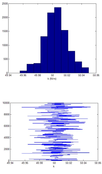
Fig. 2:M(1)- parameter estimation of linear stiffnessk(1)and history of samples
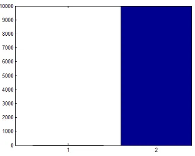
Fig.2. shows the results of applying the RJMCMC algorithm on simulated linear data using10000iterations. As expected, the algorithm chose the linear model,M(1), as more appropriate to represent the data. Fig.3. shows a bar chart of how the RJMCMC algorithm is favouring model 1 over model 2 when using linear train-ing data. The algorithm stayed in the linear model for 9999 of the times and only tried to visit the nonlinear model once.
Fig. 3: Model 1 vs Model 2 - using linear training data
Fig. 4:M(2)- parameter estimation of linear stiffnessk(2) and nonlinear stiffnessk3(2)
[image:13.595.200.394.570.725.2]Fig.5. shows a bar chart of how the RJMCMC algorithm is favouring model 2 over model 1 when using nonlinear training data. The algorithm visited the linear model only 6 times and the nonlinear one 9996 times.
5
Discussion and Conclusions
The aim of this contribution was to provide an example of using the RJMCMC algorithm on two simulated models for a SDOF system. The RJMCMC algorithm is capable of doing model selection and parameter estimation simultaneously, which makes the algorithm a desirable tool in SI of dynamical systems. Further-more, the algorithm is proven to function on nonlinear systems. In Section 4 the algorithm was used to do SI for a SDOF system for which there are two candidate models: a linear model and a nonlinear model of Duffing type. The algorithm proved successful in choosing the right model according to the data used (from a linear model or a nonlinear one). In addition, the RJMCMC algorithm identified when the nonlinearity in the second model is low enough so that the data could be represented by the first model, the linear one. This proves that the RJMCMC algorithm prevents overfitting.
In terms of future work, the authors of this current contribution are planning to find a way to tune the proposals automatically. Also, after experimental work is conducted and data is obtained, the authors plan to use the RJMCMC algorithm on real data.
Acknowledgements
The authors would like to acknowledge the ’Engineering Nonlinearity’,an EPSRC funded Programme Grant, for supporting their research (http://www.engineeringnonlinearity.ac.uk/).
References
[1] Xiao-Li Meng, G.L. Jones, A. Gelman, S. Brooks,Handbook of Markov Chain Monte Carlo, Chapman and Hall/CRC, 2011.
[2] The MathWorks 2012.Matlab R2012a., 2012.
[3] D. Barber,Bayesian Reasoning and Machine Learning, Cambridge University Press, 2012.
[4] D. Tiboaca, P.L. Green, R.J. Barthorpe, Bayesian System Identification of Dynamical Systems using Reversible Jump Markov Chain Monte Carlo, Proceedings of IMAC XXXII Conference, Orlando, FL, 2014.
[5] S.G. Razul, W.J. Fitzgerald, C. Andrieu,Bayesian model selection and parameter estimation of nuclear emission spectra using RJMCMC, Journal Nuclear Instruments and Methods in Physics Research(2002).
[6] K. Worden, G.R. Tomlinson,Nonlinearity in Structural Dynamics - Detection, Identification and Mod-elling, Institute of Physics Publishing, 2001.
[7] J. Pearl,Probabilistic Reasoning in Intelligent Systems, Morgan Kaufmann Publishers, 1988.
[8] J.-N. Juang,Applied System Identification, Prentice Hall, 1994.
[10] D.J.C. MacKay,Information Theory, Inference, and Learning Algorithms, Cambridge University Press, 2003.
[11] A. Doucet, P.M. Djuric, C. Andrieu, Model selection by MCMC computation, Journal of Signal Pro-cessing, Vol. 81, pp. 19-37.
[12] A. Doucet, C. Andrieu, Joint Bayesian Model Selection and Estimation of Noisy Sinusoids via Re-versible Jump MCMC, IEEE Transactions on Signal Processing, 1999.
[13] P.J. Green, D.I. Hastie, Model Choice using Reversible Jump Markov Chain Monte Carlo, Statistica Neerlandica, pp. 309-338, 2012.
[14] T. Baldacchino, S.R. Anderson, V. Kadirkamanathan,Computational system identification for Bayesian NARMAX modelling, Automatica, Vol. 49, pp. 2641-2651, 2013.
[15] I. Ntzoufras, J.J. Forster, P. Dellaportas, On Bayesian model and variable selection using MCMC, Statistics and Computing, Vol. 36, pp. 12-27, 2002.
[16] P.J. Green,Reversible jump Markov Chain Monte Carlo computation and Bayesian model determina-tion, Biometrika, Vol. 82, pp. 711-732, 1995.
[17] P.L. Green, K. Worden, Modelling Friction in a Nonlinear Dynamic System via Bayesian Inference, IMAC XXXI Proceedings, 2013.
[18] K. Worden, J.J. Hensman,Parameter estimation and model selection for a class of hysteretic systems using Bayesian inference, Mechanical Systems and Signal Processing, Vol. 32, pp. 153-169, 2012.
[19] Thomas Bayes,An Essay Towards Solving a Problem in the Doctrine of Chances, Philosophical Trans-actions of the Royal Society of London, Vol. 418, pp. 53-370, 1763.
[20] Stephen E. Fienberg,When did Bayesian Inference become ’Bayesian’, Bayesian Analysis, Vol. 1, pp. 1-40, 2006.