Self-commissioning Notch Filter for Active
Damping in Three Phase
LCL
-filter Based Grid-tie
converter
Rafael Pe˜na-Alzola, Marco Liserre,
Fellow, IEEE,
Frede Blaabjerg,
Fellow, IEEE,
Martin
Ordonez,
Member, IEEE,
and Tamas Kerekes,
Member, IEEE
Abstract—LCL-filters are a cost-effective solution to mitigate harmonic current content in grid-tie converters. In order to avoid stability problems, the resonance frequency ofLCL-filters can be damped with active techniques that remove dissipative elements but increase control complexity. A notch filter provides an effective solution, however tuning the filter requires considerable design effort and the variations in the grid impedance limit theLCL-filter robustness. This paper proposes a straightforward tuning procedure for a notch filter self-commissioning. In order to account for the grid inductance variations, the resonance frequency is estimated and later used for tuning the notch filter. An estimation for the maximum value of the proportional gain to excite the resonance is provided. The resonance frequency is calculated using the Goertzel algorithm, which requires little extra computational resources in the existing control processor. The Discrete Fourier Transform (DFT) coefficients are therefore obtained, with less calculations than the running sum implemen-tation and less memory requirements than with the Fast Fourier Transform (FFT). Thus, the self-commissioning technique is robust to grid impedance variations due to its ability to tune the grid-tie inverter on-site. Finally, the analysis is validated with both simulation and experiments.
Index Terms—Active damping, Autotuning, Converter control, Pulse Width Modulation (PWM).
I. INTRODUCTION
G
RID converters use either an inductor or anLCL-filter to mitigate the harmonic current content. It is well known [1]–[3] that using an LCL-filter instead of a simple inductor leads to reduced inductance values and so lower losses and volume. The LCL-filter resonance must be damped in order to avoid stability problems in the current control. For this concern, passive damping methods use series resistors that increase the encumbrances [4] and reduce the overall effi-ciency [5]. Active damping avoids dissipative elements at the expense of increased control complexity. In both cases large grid impedance variations [6]–[8] and parameter uncertainty [9] can turn the damping ineffective, challenging the LCL -filter stability.R. Pe˜na-Alzola and M. Ordonez are with the Department of Electrical and Computer Engineering, the University of British Columbia. 2332 Main Mall, Vancouver V6T 1Z4, BC Canada. E-mail:{rafaelpa,mordonez}@ece.ubc.ca
M. Liserre is the Institute for Power Electronics Electronics and Electrical Drives, Christian-Albrechts-University of Kiel, 24143 Kiel, Germany. E-mail: [email protected]
F. Blaabjerg and T. Kerekes are with Department of Energy Technology, Aalborg University. Pontoppidanstrde 101, 9220 Aalborg, Denmark. E-mail: {fbl,tak}@et.aau.dk
Active damping solution has been thoroughly studied in numerous publications [10]–[24]. An early proposal [10] adds the derivative of the grid current to the converter current control. In [11]–[13], [13]–[15] the feedback of theLCL-filter capacitor current to the voltage reference yields resonance damping. Another method consists in adding the capacitor voltage filtered by a lead-lag network [6], [16], [17] or a high-pass filter [18] to the modulator voltage reference. Robust strategies by using sliding control mode are proposed in [19], [20]. The virtual resistor method [21], [22] modifies the control algorithm to make the system behave as if there was a damping resistor without physically adding it.
Active damping by using a notch filter on the reference voltage for the modulator is simple to implement and does not need additional sensors [23]. Nevertheless, the interactions with the current control loop make the notch filter tuning a dif-ficult task. The notch tuning procedure proposed in [23] uses sophisticated genetic algorithms and the formulas proposed in [24] require numerous trial and error iterations. With the notch frequency properly tuned at the resonance frequency the voltage reference does not contain any component susceptible of exciting theLCL-filter. However, since the grid impedance variations affects the resonance frequency, the notch filter erroneous tuning will compromise the LCL-filter stability.
As the active damping is strongly dependent on the LCL -filter resonance, it is recommended to measure it on-site. The LCL-filter resonance/grid inductance estimation has already been proposed in the literature [25]–[29]. However, it cannot be embedded easily into a non-dedicated platform as the control processor may be overloaded. The estimation of the grid impedance is usually done by injecting signal at a non-characteristic frequency [26]–[29]. In [26] the frequency characteristic of theLCL-filter are used in estimating the grid impedance. In [27] the required Fourier analysis is performed using the running sum implementation of the Discrete Fourier Transform (DFT) to spare memory and calculations.
CDC
Cf
L R Lg Rg
vDC
i
v ic vc vg
[image:2.612.316.562.55.176.2]ig
Fig. 1. LCL-filter based three phase active rectifier.
resonance is provided. TheLCL-filter resonance frequency will be calculated by using Fourier analysis. In order to reduce the DSP computational and memory requirements the Goertzel algorithm is employed to calculate the Fourier coefficients. The DFT coefficients are therefore obtained, with less calcu-lations than the running sum implementation and less memory requirements than with the Fast Fourier Transform (FFT). This paper is organized as follows: §II reviews the current control methods in LCL-filters.§III explains the proposed notch filter tuning procedure. §IV deals with the resonance detection pro-cedure. §V and §VI explain the simulation and experimental results respectively. Finally, conclusions are presented in§VII.
II. CURRENT CONTROL OFLCL-FILTER GRID CONVERTER Fig. 1 shows the considered three phase LCL-filter based grid converter. The resonance frequency of the LCL-filter is:
ωres= 2πfres= √
1 Cf
( 1
L +
1 Lg
)
(1)
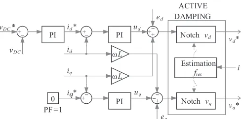
Fig. 2 shows the usual cascade control structure of the grid converter in the dq-frame. The active damping is achieved by the notch filter on the reference voltage for the modulator. Fig. 2 also shows the estimation block of the resonance frequency to tune the notch filter. In the low frequency range (ω << ωres)the capacitor branch can be neglected and theLCL-filter
behaves like an equivalent inductor with inductance Leq =
L+Lg and resistanceReq=R+Rg respectively [2]. Hence,
the PI controllers for the converter current, the one sensed in this paper, can be tuned by using the usual technical optimum criterion [16]. The integration timeTi=Leq/Req cancels the
slow dynamics and the proportional gain limits the overshoot. It is simple to deduce that the achieved gainGMlf mand phase
margin P Mlf m are respectively:
GMlf m≈π(9.94 dB) withωpc=π/(3Ts) (2)
P Mlf m ≈90◦− 270
π KpTs
Leq
withωgc=Kp/Ts (3)
where ωpc and ωgc are the phase and gain crossover
frequencies respectively and Ts is the sampling period. The
proportional gain is usually adjusted for approximately 4% overshoot with Kp=Leq/(3Ts)and soP Mlf m = 61.4◦.
+
− PI +−+
ωL
− +
PI
− −+
0 PF =1
+
− PI Notch vd
Notch vq ud
ed
uq
eq id*
id
iq
iq* vDC*
vDC
vd*
vq* ACTIVE DAMPING
ωL
Estimation
[image:2.612.53.300.57.150.2]fres i
Fig. 2. Block diagram of the converter control with active damping based on notch filter.
III. NOTCH FILTER ACTIVE DAMPING
The generic transfer function of an analog notch filter is given as [24]:
Nn(s) = (
s2+ 2D
zωnfs+ω2nf
s2+ 2D
pωnfs+ω2nf )n
(4)
where ωnf is the notch frequency, Dz and Dp are the
damping factors for the complex conjugates poles and zeros respectively and n is the number of sections. The open-loop transfer function of the converter current control in Fig. 2 for the continuous-time domain and without considering the notch filter is:
Gol(s) =GP I(s)Gd(s)G(s) (5)
where G(s) is the transfer function relating the converter voltagev and currenti,Gd(s)models the computational and
PWM delays, and finally GP I(s) is the PI controller tuned
as previously explained. The frequency that corresponds to
−180◦ phase-shift for the open-loop transfer function is near the resonance frequency [16]. In order to obtain stability with a positive gain margin the resonant peak should be below unity (0 dB). Therefore, with the inclusion of a notch filter Nn(s)
in cascade to the PI controller output it should result in:
|Gol(s)Nn(s)|s=jωres <1 (0 dB) (6) and the condition for stability isDz/Dp<|Gol(s)|−
1
s=jωres. As a digital implementation will be used for the notch filter, absolute cancellation at the resonance frequency,
|Nn(jωres)|= 0(−∞dB), is possible by settingDz= 0and
ωnf =ωres. Hence, there will be no component present in the
voltage reference able to excite the LCL-filter resonance and (6) is always fulfilled. In order to preserve the null amplitude when discretisizing (4) the bilinear transformation [4] (Tustin method) with pre-warping atω=ωnf must be used.
For frequencies much lower thanω << ωf the behavior of
the notch filter with Dz = 0 can be approximated ton first
order systems with the time constantτ= 2Dp/ωnf and using
the Taylor series the amplitude and phase are approximately:
|Nn(s)| ≈ − 40 ln(10)nD
2
p (
ω ωnf
)2
Frequency (Hz) −100
−80 −60 −40 −20 0
M
agni
tude
(dB) n=1
n=2 n=3
[image:3.612.58.292.58.170.2]2000 3000
Fig. 3. Notch filter magnitudes for increasing number of sectionsn, see (4).
⟨Nn(s)⟩ ≈ −2nDp (
ω ωnf
)
rad (8)
As the module in (7) (normalized to the resonance frequency ω/ωf << 1) decays with the squared frequency the module
of Gol(s) (5) is much less affected than the phase angle due
to the presence ofNn(s). Hence, the gain crossover frequency
ωgc of the open loop transfer function will be very close to
that of the low frequency model in (3). Conversely, the phase margin will be inferior to that of the low frequency model (3) due to the phase delay of Nn(s). The parameter Dp can
be adjusted to result in a phase margin reduction ∆P M as follows:
Dp= 1 2tan
( ∆P M
n 2π 360
) (ω′ gc
ωnf −
ωnf
ω′gc )
(9)
whereωgc′ is the crossover frequency (3) taking into account the bilinear transformation with pre-warping:
ωgc′ =ωnf
tan(ωgcTs/2) tan(ωnfTs/2)
(10)
If the notch filter width is very narrow the system is too sensible to the variations in the resonance frequency. Fig. 3 shows the notch filter amplitude for an increasing number of sections n and with the same ∆P M in (9). It can be seen that the notch width is larger for an increasing number of sections n and so the system more robust to the resonance frequency variation. Moreover, for small ∆P M and approxi-matingtanθ≈θ in (9), the module ofNn(s)decreases with
n according to (7). Hence, increasing n results in a lower intrusion in the low frequency regionω << ωf ofGol(s), see
Fig. 3. However, increasing the number of sectionsnrequires additional computations. Selecting n= 2 results in a proper compromise between the robustness and computational burden needed to implement the filter.
The low frequency dynamics of the closed-loop system behaves almost like a second order system with the phase margin P Mlf approximately related to the damping factor
according to ξ = P Mlf/100. A reduction in the phase
margin leads to a reduction in the damping factor and so an increased overshoot that may not be acceptable. Reducing the proportional gain Kp increases the phase gain achieving an
acceptable overshoot at the price of reducing the bandwidth ωbw = Kp/Leq. This reduction in the bandwidth can be
lower bound for the necessary gain reduction can be obtained from (3) by pre-compensating the resulting decrease in the phase gain∆P M:
%Kp≈100 (
1− π 90∆P M
)
(11)
Hence, the phase gain reduction ∆P M should not be selected higher than 15◦ in order not to reduce the band-width more than 50%. Thus, selecting a phase margin re-duction of no more than ∆P M = 15◦ results in a proper trade-off between robustness to the resonance variations and proper low frequency behavior. For ∆P M = 15◦ |Gol(s)|
is very little affected by Nn(s) and, as ωgc << ωpc and ∆P M = 15◦<< P Mlf m(3) the reduction in the gain margin
is small and moreover can be compensated by the gain reduction in (11).
IV. ESTIMATION OF THELCL-FILTER RESONANCE FREQUENCY
When a large grid impedance variation occurs, the reso-nance frequency changes and the notch filter is tuned at an erroneous frequency. The notch filter is not able to cancel the voltage reference components susceptible of exciting theLCL -filter and stability will be compromised. Hence, to account for the grid inductance variations, and also with variations due to aging of the passive elements, it is proposed to estimate the resonance frequency firstly and later to use it for tuning the notch filter, see Fig. 2. For this aim the resonance is excited in a controlled manner and its frequency is identified in the spectrum by using Fourier analysis [26].
Without the notch filter, the inductor resistances R and Rg provide normally passive damping which is sufficient to
achieve stability for very lowKp in the PI controller but so
little that resonance excitation will result in a large oscillation. Considering again Gol(s) in (5) and taking into account the
inductor resistances, as again the phase for the resonance frequency is near −180◦, the condition for stability resulting in a positive gain margin is:
|Gol(s)|s=jωres =|GP I(s)Gd(s)G(s)|s=jωres <1 (0 dB) (12) Neglecting the computational and PWM delays and assum-ing null the integral action of the PI controller atωres, after
some algebraic manipulation and neglecting small terms, the maximum proportional gain which results in stable control is:
Kpre=R+Rg (
L Lg
)2
(13)
This estimation (13) can be used as a guideline to gradually increase Kp until exciting the resonance but without turning
z− 1
z− 1 i(nTs) Q[n]
Q[n− 1 ]
Q[n− 2 ]
− + + +
Q[N]
Q[N− 1 ]
All samples
− + + +
2cos(2πk/N)
Each N samples
|I[k]|2
MN
samples
M
frequencies
[image:4.612.321.554.57.197.2]2cos(2πk/N)
Fig. 4. Implementation of the Goertzel algorithm for estimating the resonance frequency.
identifying the resonance frequency. The Goertzel algorithm is only more efficient than the FFT [30] for calculating M DFT coefficients when M < log2N with N the number of samples, which is not required to be a power of 2. However, its implementation is very simple, see Fig. 4. In order to calculate the k coefficient of the DFT, the DSP simply samples the converter current iand passes it through an IIR filter [30]:
Q[n] =i(nTs) + 2 cos (
2πk N
)
Q[n−1]−Q[n−2] (14) where N is the number of samples. After N samples the DFT module is calculated as [31]:
|I[k]|2=Q2[N] +Q2[N−1]−2 cos (
2πk N
)
Q[N]Q[N−1]
(15) Hence, unlike the FFT, it is not needed to storeN samples in the memory. Note that, as the phase is not needed, more computations are saved when using (15) requiring only real additions and multiplications. The process is repeated M times, one per each of the necessary DFT coefficients, and the algorithm execution time will be te = N ·M ·Ts. As
the resonance frequency is clearly predominant it is easily detected. The spectral leakage is not problematic and a rect-angular window, with resolution 2fs/N, can be used. The
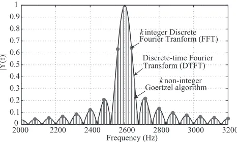
Goertzel algorithm for module calculation allows non-integer values of k = fk ·N ·Ts [32], with fk the corresponding
frequency, so arbitrary samples of the discrete time Fourier transform (DTFT) [30] can be calculated, see Fig. 5. Thus,M can be selected to obtain resolution equal to|fmax
res −fresmin|/M
with fresmax and fresmin the maximum and minimum expected resonance frequencies respectively.
If the grid impedance is inductive (no power factor cor-rection capacitor connected to the secondary of the feeding converter), once the resonance frequency is known the grid inductance value can be calculated by simply using the for-mula of the LCL-filter resonance. The Goertzel algorithm can also be used for the Fourier analysis in estimating the grid impedance on-line by injecting periodically a signal at a non-characteristic frequency.
V. SIMULATION RESULTS
Table I contains the parameters for the simulations (using Matlab/Simulink). The inductor core losses and the capacitor
20000 2200 2400 2600 2800 3000 3200 0.1
0.2 0.3 0.4 0.5 0.6 0.7 0.8 0.9 1
Frequency (Hz)
|Y
(f)|
k non-integer Goertzel algorithm k integer Discrete Fourier Tranform (FFT)
[image:4.612.53.297.57.161.2]Discrete-time Fourier Transform (DTFT)
Fig. 5. Illustration of the Goertzel algorithm for non-integerk.
TABLE I
PARAMETERS FOR THE SIMULATIONS AND EXPERIMENTS
Parameter Value
Rated powerSn 2 kW
Rated voltageVn 400 V
Rated frequencyfn 50 Hz
DC-link voltageVDC 650 V
Sampling frequencyfs 8 kHz
PWM frequencyfsw 8 kHz
Converter inductor inductanceL 1.8 mH Converter inductor resistanceR 0.1Ω Filter capacitor capacitanceCf 4.7µF Grid inductor inductanceLg 1.2 mH Grid inductor inductanceRg 0.84Ω Resonance frequencyfres 2735.93 Hz
ESR were not considered and the power switches were ideal. Without including the notch filter for active damping the system is only stable for small values of Kd. According to
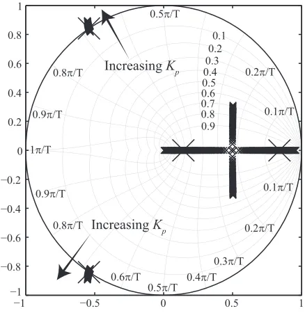
(13), the maximum proportional gain resulting in stability is Kd = 2. According to the root locus shown in Fig. 6, it is
Kd= 2.5 and, thus, (13) results in a conservative estimation.
However, in practice both estimations will be conservative as the capacitor ESR and inductor core losses were not taken into account.
Fig. 7 shows the root loci in thez-plane of the overall system with notch filter forn= 2when varying the passive elements of the LCL-filter. In Fig. 7a the inductanceL varies between 60% and 200% of the rated value. The system is stable for L >61% and remains stable for large values. In Fig. 7b the capacitanceCf varies between 70% and 200%. The system is
stable for filter capacitor values in the interval 73%< Cf < 181%. Finally, in Fig. 7 the inductance Lg varies between
20% and 300%. For small values of Lg the overall system is
stable, as it is close to the L-filter case, up to Lg > 210%
where instability occurs. It can also be seen that for increases inLgthe low frequency poles result in more damping and so
lower GM as predicted by (3).
−1 −0.5 0 0.5 1 −1
−0.5 0 0.5 1
0.9 0.7 0.5 0.3 0.1
/T
/T 0.
f g
L<100% Cf<100% L
g<100%
a) b) c)
Lg>100%
Lg<100% 0.5π/T
1π/T 1π/T
0.5π/T
−1 −0.5 0 0.5 1
−1 −0.5 0 0.5
0.1
0.3 0.5 0.7 0.9
0.5π/T 0.5π/T
1π/T 1π/T
−1 −0.5 0 0.5 1
1
−1 −0.5 0 0.5 1
0.1 0.3 0.5 0.7 0.9 0.5π/T
0.5π/T 1π/T
1π/T
Fig. 7. Root locus in thez-plane of the overall system for notch filter withn= 2when varying the passive elements: a) converter inductor L, b) filter capacitorCf and c) grid inductorLg.
−1 −0.5 0 0.5 1
−1 −0.8 −0.6 −0.4 −0.2 0 0.2 0.4 0.6 0.8 1
0.9 0.8 0.7 0.60.5 0.4 0.3
0.2 0.1
0.9π/Τ
Increasing Kp
Increasing Kp
0.8π/Τ
0.5π/Τ
0.2π/Τ
0.1π/Τ
1π/Τ
0.9π/Τ
0.8π/Τ
0.1π/Τ
0.2π/Τ
[image:5.612.53.562.55.243.2]0.3π/Τ 0.4π/Τ 0.5π/Τ 0.6π/Τ
Fig. 6. Root locus for the undamped system.
enough for small variations in the parameters. Moreover, the robustness increases for increasing n, as expected from the previous analysis, at the price of increased calculations. The robustness for n = 2 is much higher than for n = 1 and little lower than for n = 3. Hence, selecting n = 2 results in a proper trade-off between robustness and computational burden.
TABLE II
VARIATION INTERVALS RESULTING IN STABLE CONFIGURATION AND
COMPUTATIONAL REQUIREMENTS.
n %L %Cf %Lg Mults. Adds. Regs.
1 [66,-] [73,173] [-,169] 5 4 2
2 [61,-] [73,181] [-,210] 10 8 4
3 [61,-] [73,181] [-,225] 15 12 6
Frequency (Hz)
−100 −80 −60 −40 −20 0 20
M
agni
tude
(dB)
1000 −360
−315 −270 −225 −180 −135 −90 −45
P
ha
se
(de
g)
GM= 10.7 dB GM= 7.1 dB
GM= 10.8 dB
PM= 62.1º PM= 47.4º PM= 61.6 º
No damping
No damping Low freq. model
Low frequency model Notch filter
Notch filter
Notch filter and overshoot reduction
Notch filter and overshoot reduction
[image:5.612.65.284.294.519.2]2000 3000
Fig. 8. Bode plots of the converter current control.
Fig. 8 shows the Bode plots for the converter current control with no damping, the notch filter (∆P M = 15◦) and the notch filter (∆P M = 15◦) with Kp reduction for
limiting the overshoot. From Fig. 8 it can be seen that the resonant peak is completely canceled by the notch filter. As the module ofGol(s)(5) is very limitedly affected byNn(s), the
phase gain crossover frequencies for the case of no damping and the case with the notch filter are very close and the considered approximations are all valid. TheKpreduction for
4% overshoot was 65% coherent with the lower bound (11).
[image:5.612.313.567.294.503.2]5
0 0.05 0.1 0.15 0.2 0.25
−1. 5 −1 −0.5 0 0.5 1 1. 5 −1. 5 −1 −0.5 0 0.5 1 1. 5
Resonance Estimation
gri
d c
urr
. (pu)
conv
. c
urr
. (pu)
Active Damping Activation
Increase in grid Inductance Lg=200%
Lg= 300%
time (s)
Trip a)
[image:6.612.50.291.57.213.2]b)
Fig. 9. Grid current, a), and converter current, b) in simulations.
0 50(fund.) 500 1,000 1,500 2,000 2,500 3,000 3,500 4,000
0 0.05 0.101 0.15 0.20 0.25 0.30 0.35 0.30 0.45
[image:6.612.318.557.58.158.2]Frequency (Hz) Detected Resonance Frequency 2736 kHz Frequency Range for Goertzel Algorithm
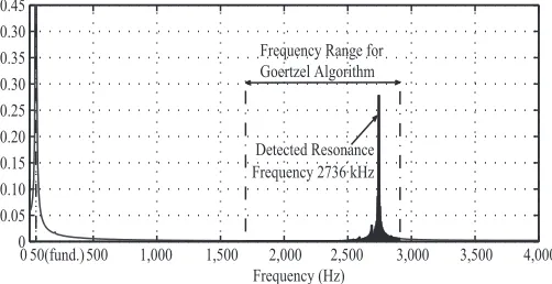
Fig. 10. Harmonic spectrum for the sampled converter current in simulations.
the harmonic content of the converter current (sampled at the switching frequency) in a certain frequency range. Fig. 10 shows the harmonic spectrum of the converter current with the frequency range calculated by using the Goertzel algorithm highlighted. The frequency range to detect the resonance is selected by assuming an infinite value for line inductance (for Lg → ∞ by calculating the limit in (1) ωres → 1/
√ CfL
) which would result in a resonance frequency of 1730.35 Hz, and an underestimated inductanceLg in the grid inductor
of 80% the rated value, which would result in a resonance frequency of 2934.96 Hz. The Goertzel algorithm estimates the resonance frequency as being 2736 Hz, an exact value because of the ideal conditions of the simulations. After calculating the needed parameters, the notch filter is connected at t = 0.05
s and it can be seen in Fig. 9 that the active damping begins. At t = 0.15 s the grid inductance Lg is increased
to 200% of the rated value and, as predicted by the previous z-plane analysis, the notch filter is robust enough to continue effectively with the active damping. Finally, at t= 0.25s the grid inductance Lg is increased to 300% of the rated value
and, as predicted by the previous z-plane, analysis the system become unstable. At this point the system will trip and the process of self-commissioning would start again by calculating the new resonance frequency for this condition.
[image:6.612.316.558.200.321.2]Fig. 11. Laboratory set-up for experiments with the three phaseLCL-filter based grid converter controlled by a dSpace system.
Fig. 12. Oscilloscope screen capture showing the inverter current (lower channel, time base 10 ms/div) and its FFT (upper channel).
VI. EXPERIMENTAL RESULTS
The experimental set-up has the same parameters as in Table I and is shown Fig. 11. It consists of one 2.2 kW Danfoss FC302 converter connected to the grid through an isolating transformer whose leakage inductance is Lg. The DC-link is
established by a Delta Elektronika DC-power source and the control algorithm has been implemented in a dSPACE DS1103 real time system.
Fig. 12 shows an oscilloscope screen capture for the con-verter current and its Fourier spectrum when the resonance is being excited. The Goertzel algorithm with N = 100 and M = 300 takes 3.75 s and detects the resonance frequency variations within the span of 1700-2900 Hz, see Fig. 13. The detected resonance frequency is 2695 Hz according to the Goertzel algorithm implemented in the dSpace systems, see Fig. 13, and 2699 Hz according to oscilloscope FFT, see Fig. 12. Once the resonance frequency is detected all the parameters of the notch filter are calculated and upon connection the active damping starts, see Fig. 14, when the oscillations are effectively damped.
[image:6.612.49.300.261.390.2]0 0.5 1 1.5 2 2.5 3 3.5 4 1.6
1.8 2.0 2.2 2.4 2.6 2.8
fre
que
nc
y (kH
z
)
time (s)
[image:7.612.64.289.60.208.2]Detected Resonance Frequency 2695 Hz
Fig. 13. Frequency swept (dashed line) for detecting the resonance frequency (full line) using the Goertzel algorithm.
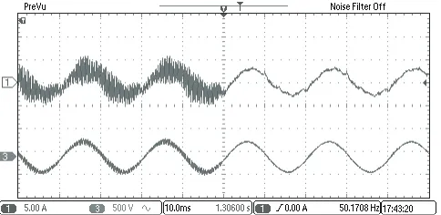
Fig. 14. Oscilloscope screen capture for the grid current (upper channel) and capacitor voltage (lower channel) upon the connection of the notch filter.
VII. CONCLUSION
This paper presented a self-commissioning technique for active damping that provides the ability to tune on-site the grid-tie inverter. The provided formulas for tuning the notch filter are straightforward and require no trial-and-error it-erations. The notch filter results in robust active damping for medium variations in the resonance frequency due to rated parameter inaccuracies or component aging. Detecting the resonance frequency by using the Goertzel algorithm requires reduced computational and memory resources in the control processor. For large grid inductance variations, the self-commissioning procedure detects the new resonance frequency and re-tunes the the notch filter appropriately. Hence, the proposed procedure results in a robust solution for active damping of theLCL-filter based grid-tie converter and allows to exploit the attractive features of the notch filter method, simple implementation and no extra sensors.
REFERENCES
[1] F. B. M. Liserre and A. Dell’Aquila, “Step-by-step design procedure for a grid-connected three-phase pwm voltage source converter,”Int. J. of Electron., vol. 91, no. 8, pp. 445–460, 2004.
[2] M. Liserre, F. Blaabjerg, and S. Hansen, “Design and control of an lcl-filter-based three-phase active rectifier,”IEEE Trans. Ind. Applicat., vol. 41, no. 5, pp. 1281–1291, 2005.
[3] J. Muhlethaler, M. Schweizer, R. Blattmann, J. Kolar, and A. Ecklebe, “Optimal design of lcl harmonic filters for three-phase pfc rectifiers,” IEEE Trans. Power Electron., vol. 28, no. 7, pp. 3114–3125, 2013.
an lcl-filter based three-phase active rectifier,” in2002 IEEE 33rd Annu. Power Electron. Specialists Conf. PESC’02, vol. 3, 2002, pp. 1195–1201 vol.3.
[5] R. Pe˜na Alzola, M. Liserre, F. Blaabjerg, R. Sebastian, J. Dannehl, and F. Fuchs, “Analysis of the passive damping losses in lcl-filter-based grid converters,”IEEE Trans. Power Electron., vol. 28, no. 6, pp. 2642–2646, 2013.
[6] M. Liserre, R. Teodorescu, and F. Blaabjerg, “Stability of grid-connected pv inverters with large grid impedance variation,” inIEEE 35th Annu. Power Electron. Specialists Conf. PESC’04, vol. 6, 2004, pp. 4773–4779 Vol.6.
[7] J. He, Y. W. Li, D. Bosnjak, and B. Harris, “Investigation and active damping of multiple resonances in a parallel-inverter-based microgrid,” IEEE Trans. Power Electron., vol. 28, no. 1, pp. 234–246, 2013. [8] D. Yang, X. Ruan, and H. Wu, “Impedance shaping of the grid-connected
inverter with lcl filter to improve its adaptability to the weak grid condition,”IEEE Trans. on Power Electron., vol. PP, no. 99, pp. 1–1, 2014.
[9] L. Maccari, J. Massing, L. Schuch, C. Rech, H. Pinheiro, R. Oliveira, and V. Montagner, “Lmi-based control for grid-connected converters with lcl filters under uncertain parameters,” IEEE Trans. Power Electron., vol. PP, no. 99, pp. 1–1, 2013.
[10] A. Hava, T. Lipo, and W. L. Erdman, “Utility interface issues for line connected pwm voltage source converters: a comparative study,” inProc. Appl. Power Electron. Conf. and Expo., 1995 APEC’95, no. 0, 1995, pp. 125–132 vol.1.
[11] Y. Tang, P. C. Loh, P. Wang, F. H. Choo, F. Gao, and F. Blaabjerg, “Generalized design of high performance shunt active power filter with output lcl filter,”IEEE Trans. Ind. Electron., vol. 59, no. 3, pp. 1443– 1452, 2012.
[12] J. Dannehl, C. Wessels, and F. Fuchs, “Limitations of voltage-oriented pi current control of grid-connected pwm rectifiers with lcl filters,”IEEE Trans. Ind. Electron., vol. 56, no. 2, pp. 380–388, 2009.
[13] C. Bao, X. Ruan, X. Wang, W. Li, D. Pan, and K. Weng, “Step-by-step controller design for lcl-type grid-connected inverter with capacitor current-feedback active-damping,”IEEE Trans. Power Electron., vol. 29, no. 3, pp. 1239–1253, 2014.
[14] D. Pan, X. Ruan, C. bao, W. Li, and X. Wang, “Capacitor-current-feedback active damping with reduced computation delay for improving robustness of lcl-type grid-connected inverter,” IEEE Trans. Power Electron., vol. PP, no. 99, pp. 1–1, 2013.
[15] Y.-R. Mohamed, M. A-Rahman, and R. Seethapathy, “Robust line-voltage sensorless control and synchronization of lcl -filtered distributed generation inverters for high power quality grid connection,” IEEE Trans. Power Electron., vol. 27, no. 1, pp. 87–98, 2012.
[16] V. Blasko and V. Kaura, “A novel control to actively damp resonance in input lc filter of a three-phase voltage source converter,”IEEE Trans. Ind. Applicat., vol. 33, no. 2, pp. 542–550, 1997.
[17] R. Pe˜na Alzola, M. Liserre, F. Blaabjerg, R. Sebastian, J. Dannehl, and F. Fuchs, “Systematic design of the lead-lag network method for active damping in lcl-filter based three phase converters,” IEEE Trans. Ind. Informat., vol. PP, no. 99, pp. 1–1, 2013.
[18] M. Malinowski and S. Bernet, “A simple voltage sensorless active damping scheme for three-phase pwm converters with an lcl filter,”IEEE Trans. Ind. Electron., vol. 55, no. 4, pp. 1876–1880, 2008.
[19] X. Hao, X. Yang, T. Liu, L. Huang, and W. Chen, “A sliding-mode controller with multiresonant sliding surface for single-phase grid-connected vsi with an lcl filter,”IEEE Trans. Power Electron., vol. 28, no. 5, pp. 2259–2268, 2013.
[20] F. Fuchs, J. Dannehl, and F. Fuchs, “Discrete sliding mode current control of grid-connected three-phase pwm converters with lcl filter,” in2010 IEEE Int. Symp. on Ind. Electron. ISIE, 2010, pp. 779–785. [21] P. Dahono, “A control method to damp oscillation in the input lc
filter,” inProc. 2002 IEEE 33rd Annu. Power Electron. Specialists Conf. PESC’02, vol. 4, 2002, pp. 1630–1635.
[22] J. He and Y. W. Li, “Generalized closed-loop control schemes with embedded virtual impedances for voltage source converters with lc or lcl filters,”IEEE Trans. Power Electron., vol. 27, no. 4, pp. 1850–1861, 2012.
[23] M. Liserre, A. Aquila, and F. Blaabjerg, “Genetic algorithm-based design of the active damping for an lcl-filter three-phase active rectifier,”IEEE Trans. Power Electron., vol. 19, no. 1, pp. 76–86, 2004.
[image:7.612.55.297.251.369.2][25] N. Hoffmann and F. Fuchs, “Minimal invasive equivalent grid impedance estimation in inductive-resistive power networks using extended kalman filter,”IEEE Trans. Power Electron., vol. 29, no. 2, pp. 631–641, 2014. [26] M. Liserre, F. Blaabjerg, and R. Teodorescu, “Grid impedance estimation via excitation of lcl -filter resonance,” IEEE Trans. Ind. Applicat., vol. 43, no. 5, pp. 1401–1407, 2007.
[27] L. Asiminoaei, R. Teodorescu, F. Blaabjerg, and U. Borup, “A digital controlled pv-inverter with grid impedance estimation for ens detection,” IEEE Trans. Power Electron., vol. 20, no. 6, pp. 1480–1490, 2005. [28] D. Reigosa, F. Briz, C. Charro, P. Garcia, and J. Guerrero, “Active
islanding detection using high-frequency signal injection,”IEEE Trans. Ind. Applicat., vol. 48, no. 5, pp. 1588–1597, 2012.
[29] M. Sumner, B. Palethorpe, and D. W. P. Thomas, “Impedance measure-ment for improved power quality-part 1: the measuremeasure-ment technique,” IEEE Trans. Power Delivery, vol. 19, no. 3, pp. 1442–1448, 2004. [30] A. V. Oppenheim, R. W. Schafer, and J. Buck, Discrete-Time Signal
Processing, 2nd ed. Prentice-Hall, 1999.
[31] S. Kuo and B. Lee,Real-Time Digital Signal Processing, 1st ed. Wiley, 2001.