Convergence rate of numerical solutions to SFDEs with jumps

(2011) Convergence rate of numerical solutions to SFDEs with jumps.

Journal of Computational and Applied Mathematics, 236 (2). pp. 119-131.

ISSN 0377-0427 , http://dx.doi.org/10.1016/j.cam.2011.05.043

This version is available at

https://strathprints.strath.ac.uk/36920/

Strathprints

is designed to allow users to access the research output of the University of

Strathclyde. Unless otherwise explicitly stated on the manuscript, Copyright © and Moral Rights

for the papers on this site are retained by the individual authors and/or other copyright owners.

Please check the manuscript for details of any other licences that may have been applied. You

may not engage in further distribution of the material for any profitmaking activities or any

commercial gain. You may freely distribute both the url (https://strathprints.strath.ac.uk/) and the

content of this paper for research or private study, educational, or not-for-profit purposes without

prior permission or charge.

Any correspondence concerning this service should be sent to the Strathprints administrator:

[email protected]

The Strathprints institutional repository (https://strathprints.strath.ac.uk) is a digital archive of University of Strathclyde research outputs. It has been developed to disseminate open access research outputs, expose data about those outputs, and enable the

Contents lists available atScienceDirect

Journal of Computational and Applied

Mathematics

journal homepage:www.elsevier.com/locate/cam

Convergence rate of numerical solutions to SFDEs with jumps

Jianhai Bao

a,∗

, Björn Böttcher

b

, Xuerong Mao

c

, Chenggui Yuan

a

a_{Department of Mathematics, Swansea University, Swansea SA2 8PP, UK}

b_{Department of Mathematics, Dresden University of Technology, 01062 Dresden, Germany}

c_{Department of Statistics and Modelling Science, University of Strathclyde, Glasgow G1 1XH, UK}

a r t i c l e i n f o

Article history:

Received 12 October 2010

Received in revised form 26 April 2011

MSC:

65C30 65L20 60H35

Keywords:

Euler–Maruyama Local Lipschitz condition SFDE

Convergence rate Poisson process

a b s t r a c t

In this paper, we are interested in numerical solutions of stochastic functional differential equations with jumps. Under a global Lipschitz condition, we show that thepth-moment convergence of Euler–Maruyama numerical solutions to stochastic functional differential equations with jumps has order 1/pfor anyp ≥ 2. This is significantly different from the case of stochastic functional differential equations without jumps, where the order is 1/2 for anyp≥2. It is therefore best to use the mean-square convergence for stochastic functional differential equations with jumps. Moreover, under a local Lipschitz condition, we reveal that the order of mean-square convergence is close to 1/2, provided that local Lipschitz constants, valid on balls of radiusj, do not grow faster than logj.

©2011 Elsevier B.V. All rights reserved.

1. Introduction

Recently, the theory of Functional Differential Equations (FDEs) has received a great deal of attention. Hale and Lune [1] have studied deterministic FDEs and their stability. For Stochastic Functional Differential Equations (SFDEs), here we highlight the great contribution of Kolmanovskii and Nosov [2] and Mao [3]. Kolmanovskii and Nosov [2] not only established the theory of existence and uniqueness of SFDEs but also investigated the stability and asymptotic stability of the equations, while Mao [3] studied the exponential stability of the equations.

On the other hand, Stochastic Differential Equations (SDEs) with jumps have been widely used in many branches of science and industry, in particular, in economics, finance and engineering (see, e.g., [4–6] and the references therein). Since most SDEs with jumps cannot be solved explicitly, numerical methods have become essential. Under a local Lipschitz condition, Higham and Kloeden [7] showed strong convergence and nonlinear stability for Euler–Maruyama (EM) numerical solutions to SDEs with jumps, while, in [8], Higham and Kloeden further revealed strong convergence rate for Backward

EMon SDEs with jumps, provided that the drift coefficient obeys a one-side Lipschitz condition and a polynomial growth condition.

Returning to SFDEs, under a local Lipschitz condition, Mao [9] showed strong convergence ofEMnumerical solutions, while revealing convergence rate under a global Lipschitz condition. To the best of our knowledge there has been no systematic work so far on numerical methods for SFDEs with jumps. The purpose of this paper is to take some steps in this direction, building extensively on the results of Mao [9] and Yuan and Mao [10] in the Brownian motion case. In reference to the existing results in the literature, our contributions are as follows:

∗_{Corresponding author.}

E-mail address:[email protected](J. Bao).

0377-0427/$ – see front matter©2011 Elsevier B.V. All rights reserved.

•

Under a global Lipschitz condition, we show that thepth-moment convergence ofEMnumerical solutions to SFDEs with jumps has order 1

/

pfor anyp

≥

2. This is significantly different from the case of SFDEs without jumps, where the order is 1

/

2 for anyp

≥

2. In practice, it is therefore best to use the mean-square convergence for SFDEs with jumps.

•

Under a local Lipschitz condition, Mao [9] showed strong convergence without rate ofEMnumerical solutions to SFDEs without jumps. However, in this work we shall reveal that the order of the mean-square convergence is close to 1

/

2, provided that local Lipschitz constants, valid on balls of radiusj, do not grow faster than logj. More precisely, the order of the mean-square convergence is 1

/(

2

+

ϵ)

, provided that local Lipschitz constants do not grow faster than

(

logj

)

1/(1+ϵ)_.

•

Some new techniques are developed to cope with the difficulties due to the jumps.

This paper is organized as follows: Section2gives some preliminary results, in particular,EMnumerical solutions to SFDEs with jumps are set up. In Section3, we discuss thepth-moment convergence ofEMnumerical solutions to SFDEs with jumps under a global Lipschitz condition. The rate of the mean-square convergence forEMnumerical solutions to SFDEs with jumps under a local Lipschitz condition is provided in Section4. Finally, in order to make the paper self-contained, an existence-and-uniqueness result of solutions to SFDEs with jumps is provided in theAppendix.

2. Preliminaries

Throughout this paper, we let

{

Ω

,

F

_,

{

F_t

}

t≥0

,

P

}

be a complete probability space with a filtration

{

Ft

}

t≥0satisfying the

usual conditions (i.e., it is continuous on the right andF_{0contains all}P-zero sets). Let

| · |

denote the Euclidean norm and the matrix trace norm. Let

τ >

0 andD

:=

D

(

[−

τ ,

0

];

Rn

₎

_{denote the family of all right-continuous functions with left-hand}

limits

ϕ

from

[−

τ ,

0

]

toRn

_,

_andD

_ˆ

_{:= ˆ}

_D

₍

_[−

_{τ ,}

₀

_];

_Rn

₎

_{denote the family of all left-continuous functions with right-hand}

limits

ϕ

from

[−

τ ,

0

]

toRn_{, we will always use}

_‖

_ϕ

_{‖ :=}

_sup

−τ≤θ≤0

|

ϕ(θ )

|

to denote the norm inDandD

ˆ

potentially involved

when no confusion possibly arises. Db

F

0

(

[−

τ ,

0

];

R

n

₎

_{denotes the family of all almost surely bounded,F}

0-measurable,

D-valued random variables. For allt

≥

0,xt

:= {

x

(

t

+

θ )

: −

τ

≤

θ

≤

0

}

is regarded as aD-valued stochastic process.

Letx

(

t−

)

:=

lims↑tx

(

s

)

ont

≥ −

τ

andxt−

:= {

x

(

t

+

θ )

−

: −

τ

≤

θ

≤

0

}

. It is easy to see thatx

(

t−

)

is aD

ˆ

-valued stochastic

process.

It should be pointed out that spaceDandD

ˆ

are not complete under the supremum norm

‖ · ‖

. To makeDa complete space, we need to define the following metric (see [11, Chapter 3]). LetΛdenote the class of strictly increasing, continuous mapping of

[−

τ ,

0

]

onto itself and

Λ∗_ϵ

=



λ

∈

Λ

:

sup

s̸=t









log

λ(

t

)

−

λ(

s

)

t

−

s









≤

ϵ



,

define

d

(ξ , ζ )

=

inf



ϵ >

0

: ∃

λ

∈

Λ∗_ϵsuch that sup

t∈[−τ ,0]

|

ξ (

t

)

−

ζ (λ(

t

))

| ≤

ϵ



.

(2.1)

d

(

·

,

·

)

is called a Skorohod metric, and by [11, Theorem 14.2, p115] we know thatDis complete in the metricd

.

Since the supremum norm and the Skorohod metric are equivalent (see [11, Theorem 14.1, p114]), we shall use the supremum norm for studying the convergence, however, we use the Skorohod metric to investigate the existence and uniqueness of the equations inAppendix.

In this paper, we consider the following SFDE with jumps

dx

(

t

)

=

f

(

xt

)

dt

+

g

(

xt

)

dB

(

t

)

+

h

(

xt−

)

dN

(

t

),

0

≤

t

≤

T

,

(2.2)

with the initial datax0

=

ξ

∈

DbF₀

(

[−

τ ,

0

];

R

n

₎

_{. Here,f}

_,

_h

_{: ˆ}

_D

_→

_Rn_,g

_{: ˆ}

_D

_→

_Rn×m_,B

₍

_t

₎

_{is anm-dimensional Brownian}

motion andN

(

t

)

is a scalar Poisson process with intensity

λ

. We further assume thatB

(

t

)

andN

(

t

)

are independent. It should be pointed out that the solution of Eq.(2.2)is inD.

For our purposes, we need the following assumptions which can also guarantee the existence and uniqueness of solution to(2.2)(seeAppendix).

(H1) (Global Lipschitz condition) There exists a left-continuous nondecreasing function

µ

: [−

τ ,

0

] →

R+such that for all

ϕ, ψ

∈ ˆ

D

|

f

(ϕ)

−

f

(ψ )

|

2

_{∨ |}

_g

_(ϕ)

₋

_g

_{(ψ )}

_|

2

_{∨ |}

_h

_(ϕ)

₋

_h

_{(ψ )}

_|

2

_≤

∫

0

−τ

|

ϕ(θ )

−

ψ (θ )

|

2_d

_{µ(θ ).}

_(2.3)

Remark 2.1. For simplicity, we writeL

:=

µ(

0

)

−

µ(

−

τ )

, which is referred to as the global Lipschitz constant. Note from

(2.3)that for all

ϕ, ψ

∈ ˆ

D

This further implies the linear growth condition, that is, for

ϕ

∈ ˆ

D

|

f

(ϕ)

|

2

∨ |

g

(ϕ)

|

2

∨ |

h

(ϕ)

|

2

≤

K

(

1

+ ‖

ϕ

‖

2

),

(2.5)

whereK

:=

2

(

L

∨ |

f

(

0

)

|

2

_{∨ |}

_g

₍

₀

₎

_|

2

_{∨ |}

_h

₍

₀

₎

_|

2

₎

_.

(H2) (Continuity of initial data) For

ξ

∈

Db

F₀

(

[−

τ ,

0

];

R

n

₎

_{and somep}

_≥

_{2, there is a constant}

_{β >}

_{0 such that}

E



|

ξ (

s

)

−

ξ (

t

)

|

p



≤

β

|

t

−

s

|

,

t

,

s

∈ [−

τ ,

0

]

.

(2.6)

For givenT

≥

0 and

τ >

0, the time-step size

△ ∈

(

0

,

1

)

is defined by

△ :=

τ

N

=

T M

with some integersN

> τ

andM

>

T. Following [9], theEMmethod applied to(2.2)produces approximationsy

¯

(

k

△

)

≈

x

(

k

△

)

by settingy

¯

(

k

△

)

:=

ξ (

k

△

),

−

N

≤

k

≤

0, and

¯

y

((

k

+

1

)

△

)

= ¯

y

(

k

△

)

+

f

(

y

¯

k△

)

△ +

g

(

y

¯

k△

)

△

Bk

+

h

(

¯

yk△

)

△

Nk

,

(2.7)

where

△

B_k

:=

B

((

k

+

1

)

△

)

−

B

(

k

△

)

is a Brownian increment,

△

N_k

:=

N

((

k

+

1

)

△

)

−

N

(

k

△

)

is a Poisson increment, and

¯

yk△

:= {¯

yk△

(θ )

: −

τ

≤

θ

≤

0

}

is aD-valued random variable defined by

¯

yk△

(θ )

:=

(

i

+

1

)

△ −

θ

△

y

¯

((

k

+

i

)

△

)

+

θ

−

i

△

△

y

¯

((

k

+

i

+

1

)

△

)

(2.8)

fori

△ ≤

θ

≤

(

i

+

1

)

△

,i

= −

N

,

−

(

N

−

1

), . . . ,

−

1, where in order fory

¯

−△to be well defined, we sety

¯

(

−

(

N

+

1

)

△

)

=

ξ (

−

N

△

)

.

Given the discrete-time approximation

{¯

y

(

k

△

)

}

k≥0, we define a continuous-time approximationy

(

t

)

by settingy

(

t

)

:=

ξ (

t

)

for

−

τ

≤

t

≤

0, while fort

∈ [

0

,

T

]

y

(

t

)

=

ξ (

0

)

+

∫

t

0

f

(

y

¯

s

)

ds

+

∫

t

0

g

(

y

¯

s

)

dB

(

s

)

+

∫

t

0

h

(

y

¯

s−

)

dN

(

s

),

(2.9)

where

¯

y_t−

:=

lim s↑t

¯

ys

,

¯

yt

:=

M−1

−

k=0

¯

yk△I[k△,(k+1)△)

(

t

).

It is easy to see thaty

(

k

△

)

= ¯

y

(

k

△

)

fork

= −

N

,

−

N

+

1

, . . . ,

M. That is, the discrete-time and continuous-timeEM

numerical solutions coincide at the gridpoints.

Remark 2.2. It is easy to observe from(2.8)that

‖¯

yk△

‖ =

max

−N≤i≤0

|¯

y

((

k

+

i

)

△

)

|

,

k

= −

1

,

0

,

1

, . . . ,

M

−

1

,

(2.10)

which further yields

‖¯

yk△

‖ ≤ ‖

yk△

‖

,

k

= −

1

,

0

,

1

, . . . ,

M

−

1

,

byy

(

k

△

)

= ¯

y

(

k

△

)

and for anyt

∈ [

0

,

T

]

‖¯

yt

‖ = ‖¯

y[t

△]△

‖ ≤ ‖

y[△t]△

‖ ≤

₋sup_τ≤s≤t

|

y

(

s

)

|

,

(2.11)

where

[

t

△

]

is the integer part of

t

△.

3. Convergence rate under global Lipschitz condition

In this section, we shall investigate convergence rate ofEMnumerical scheme under global Lipschitz condition(2.3). Our results reveal a significant difference from these on the SFDEs without jumps.

Lemma 3.1. Under condition(2.5), for

‖

ξ

‖

p

_<

_∞

_,

_p

_≥

_{2, there exists a positive constant H}

₍

_p

₎

_:=

_H

₍

_p

_,

_T

_{, ξ ,}

_K

₎

_{such that}

E



sup

−τ≤t≤T

|

x

(

t

)

|

p



∨

E



sup

−τ≤t≤T

|

y

(

t

)

|

p



Proof. Since the arguments of the moment bounds for the exact and continuous approximate solutions to(2.2)are very similar, here we only give an estimate for the continuous approximate solutiony

(

t

)

. For every integerR

≥

1, define a stopping time

θ

R

:=

inf

{

t

≥

0

: ‖

yt

‖

>

R

}

.

It is easy to see from(2.9)that for anyt

∈ [

0

,

T

]

E



sup

0≤s≤t

|

y

(

s

∧

θ

R

)

|

p



≤

4p−1

[

E

‖

ξ

‖

p

+

E



sup

0≤s≤t









∫

s 0

f

(

y

¯

r∧θR

)

dr









p



+

E



sup

0≤s≤t









∫

s 0

g

(

y

¯

r∧θR

)

dB

(

r

)









p



+

E



sup

0≤s≤t









∫

s 0

h

(

y

¯

(r∧θR)−

)

dN

(

r

)









p

]

.

(3.2)

By the Hölder inequality and(2.5)

E



sup

0≤s≤t









∫

s 0

f

(

y

¯

r∧θR

)

dr









p



≤

Tp−1

∫

t

0

E

|

f

(

y

¯

r∧θR

)

|

pdr

≤

Tp−1

∫

t

0

E

[

K

(

1

+ ‖¯

y_r∧θR

‖

2

)

]

p 2_dr

≤

2p2−1TpKp2

+

₂ p

2−1Tp−1Kp2

∫

t

0

E

‖¯

yr∧θR

‖

pdr

.

This, together with(2.11), immediately reveals that

E



sup

0≤s≤t









∫

s 0

f

(

y

¯

r∧θR

)

dr









p



≤

c1T

+

c1

∫

t

0

E



sup

−τ≤r≤s

|

y

(

r

∧

θ

R

)

|

p



ds

,

(3.3)

where c1

=

2

p

2−1Tp−1Kp2. Now, using the Burkholder–Davis–Gundy inequality [3, Theorem 7.3, p40] and the Hölder

inequality, we deduce that there exists a positive constantcpsuch that

E



sup

0≤s≤t









∫

s 0

g

(

y

¯

r∧θR

)

dB

(

r

)









p



≤

cpE

∫

t

0

|

g

(

y

¯

r∧θR

)

|

2dr



p/2

≤

cpT p−2

2

∫

t

0

E

|

g

(

y

¯

r∧θR

)

|

pdr

.

In the same way as(3.3)was done, it then follows easily that

E



sup

0≤s≤t









∫

s 0

g

(

y

¯

_r∧θR

)

dB

(

r

)









p



≤

c2T

+

c2

∫

t

0

E



sup

−τ≤r≤s

|

y

(

r

∧

θ

R

)

|

p



ds

,

where c2

=

2

p

2−1Tp−22Kp2cp. Moreover, observing thatN

˜

(

t

)

=

N

(

t

)

−

λ

t

,

t

≥

0 is a martingale measure, using the

Burkholder–Davis–Gundy inequality [12, Theorem 48, p193], Hölder inequality and(2.5), we obtain for some positive constantc

¯

p,

E



sup

0≤s≤t









∫

s 0

h

(

¯

y_(r∧θR)−

)

dN

(

r

)









p



≤

E



sup

0≤s≤t









∫

s 0

h

(

y

¯

_(r∧θR)−

)

dN

˜

(

r

)

+

λ

∫

s

0

h

(

y

¯

r∧θR

)

dr









p



≤

2p

[

E



sup

0≤s≤t









∫

s 0

h

(

y

¯

(r∧θR)−

)

dN

˜

(

r

)









p

+

λ

p sup

0≤s≤t









∫

s 0

h

(

y

¯

r∧θR

)

dr









p

]

≤

2p



¯

cp

λ

p/2E

∫

t

0

|

h

(

y

¯

r∧θR

)

|

2dr



p/2

+

λ

pTp−1

∫

t

0

E

|

h

(

y

¯

r∧θR

)

|

pdr



≤

c3T

+

c3

∫

t

0

E



sup

−τ≤r≤s

|

y

(

r

∧

θ

R

)

|

p



ds

,

wherec3

=

2

3p 2−1Kp2



¯

cp

λ

p/2T

p−2

2

+

_λ

pTp−1



. Hence, in(3.2)

E



sup

0≤s≤t

|

y

(

s

∧

θ

R

)

|

p



≤

4p−1

[

E

‖

ξ

‖

p

₊

₍

_c

1

+

c2

+

c3

)

T

+

(

c1

+

c2

+

c3

)

∫

t

0

E



sup

−τ≤r≤s

|

y

(

r

∧

θ

R

)

|

p



ds

]

Note that

E



sup

−τ≤s≤t

|

y

(

s

∧

θ

R

)

|

p



≤

E

‖

ξ

‖

p

₊

_E



sup

0≤s≤t

|

y

(

s

∧

θ

R

)

|

p



.

Applying the Gronwall inequality and lettingR

→ ∞

, we then obtain

E



sup

−τ≤t≤T

|

y

(

t

)

|

p



≤

H

(

p

).

SinceTis any fixed positive number, the required assertion follows.

In order to obtain our main results, we need to estimate thepth moment ofy

(

s

+

θ )

− ¯

ys

(θ ).

Lemma 3.2. Let conditions(2.5)and(2.6)hold. Then, for p

≥

2and s

∈ [

0

,

T

]

E

|

y

(

s

+

θ )

− ¯

ys

(θ )

|

p

≤

γ

△

,

−

τ

≤

θ

≤

0

,

(3.4)

where

γ

is a positive constant independent of

△

.

Proof. Fixs

∈ [

0

,

T

]

and

θ

∈ [−

τ ,

0

]

. Letks

∈ {

0

,

1

,

2

,

· · ·

,

M

−

1

}

,kθ

∈ {−

N

,

−

N

+

1

, . . . ,

−

1

}

be the integers for which s

∈ [

ks

△

, (

ks

+

1

)

△

)

,

θ

∈ [

kθ

△

, (

kθ

+

1

)

△

)

, respectively. For convenience, we write

v

=

s

+

θ

andkv

=

ks

+

kθ. Clearly,

0

≤

s

−

ks

△

<

△

and 0

≤

θ

−

kθ

△ ≤ △

, so

0

≤

v

−

kv

△

<

2

△

.

Recalling the definition ofy

¯

s

,

s

∈ [

0

,

T

]

, we then obtain from(2.8)that

¯

ys

(θ )

= ¯

yks△

(θ )

= ¯

y

(

kv

△

)

+

θ

−

kθ

△

△

[¯

y

((

kv

+

1

)

△

)

− ¯

y

(

kv

△

)

]

,

which implies

E

|

y

(

s

+

θ )

− ¯

ys

(θ )

|

p

≤

2p−1E

|¯

y

((

kv

+

1

)

△

)

− ¯

y

(

kv

△

)

|

p

+

2p−1E

|

y

(v)

− ¯

y

(

kv

△

)

|

p

.

(3.5)

Forkv

≤ −

1, it thus follows from(2.6)that

E

|¯

y

((

kv

+

1

)

△

)

− ¯

y

(

kv

△

)

|

p

≤

β

△

.

(3.6)

Note that for someH

¯

:= ¯

H

(

m

,

p

)

E

|

B

(

t

)

|

p

_{≤ ¯}

_Htp₂

_,

_t

_≥

₀

_,

_(3.7)

and, by the characteristic functions’ argument, for

△ ∈

(

0

,

1

)

E

|△

Nk

|

p

≤

C

△

,

(3.8)

whereCis a positive constant which is independent of

△

. Fork_v

≥

0, using(2.7)and notingg

(

y

¯

_kv△

)

andBkv

,

h

(

y

¯

kv△

)

and

Nkvare independent, respectively, we compute

E

|¯

y

((

kv

+

1

)

△

)

− ¯

y

(

kv

△

)

|

p

≤

3p−1



E

|

f

(

y

¯

kv△

)

|

p

△

p

+

E

|

g

(

y

¯

kv△

)

|

pE

|△

Bkv

|

p

+

E

|

h

(

y

¯

kv△

)

|

pE

|△

Nkv

|

p



.

Taking(2.5)into consideration and applyingLemma 3.1, we then obtain that for

△ ∈

(

0

,

1

)

E

|¯

y

((

kv

+

1

)

△

)

− ¯

y

(

kv

△

)

|

p

≤

3p−12 p

2−1Kp2

₍

₁

+

H

(

p

))(

1

+ ¯

H

+

C

)

△

.

(3.9) Hence, in(3.5)

E

|

y

(

s

+

θ )

− ¯

ys

(θ )

|

p

≤

2p−1

β

+

3p−12 3p

2−2Kp2

₍

₁

+

H

(

p

))(

1

+ ¯

H

+

C

)

△ +

2p−1E

|

y

(v)

− ¯

y

(

kv

△

)

|

p

.

(3.10)

In what follows, we divide the following five cases to estimate the second term on the right-hand side of(3.10).

Case1:kv

≥

0 and 0

≤

v

−

kv

△

<

△

. By(2.9)

E

|

y

(v)

− ¯

y

(

kv

△

)

|

p

=

E

|

f

(

y

¯

kv△

)(v

−

kv

△

)

+

g

(

y

¯

kv△

)(

B

(v)

−

B

(

kv

△

))

+

h

(

y

¯

kv△

)(

N

(v)

−

N

(

kv

△

))

|

p

≤

3p−1

E

|

f

(

y

¯

kv△

)

|

p

(v

−

kv

△

)

p

+

3p−1E

|

g

(

y

¯

kv△

)

|

pE

|

B

(v)

−

B

(

kv

△

)

|

p

+

3p−1E

|

h

(

y

¯

kv△

)

|

p_E

_|

_N

_(v)

₋

_N

₍

_k v

△

)

|

p

.

Then, in the same way as(3.9)was done, we have for

△ ∈

(

0

,

1

)

E

|

y

(v)

− ¯

y

(

kv

△

)

|

p

≤

3p−12 p 2−1_K

p

Case2:kv

≥

0 and

△ ≤

v

−

kv

△

<

2

△

. It then follows easily that

E

|

y

(v)

− ¯

y

(

k_v

△

)

|

p

₌

_E

_|

_y

_(v)

_{− ¯}

_y

₍₍

_k

v

+

1

)

△

)

+ ¯

y

((

kv

+

1

)

△

)

− ¯

y

(

kv

△

)

|

p

≤

2p−1_E

_|

_y

_(v)

_{− ¯}

_y

₍₍

_k

v

+

1

)

△

)

|

p

+

2p−1E

|¯

y

((

kv

+

1

)

△

)

− ¯

y

(

kv

△

)

|

p

.

This, together with(3.9)and Case 1, leads to

E

|

y

(v)

− ¯

y

(

kv

△

)

|

p

≤

3p−12 3p

2−1Kp2

₍

₁

+

H

(

p

))(

1

+ ¯

H

+

C

)

△

.

Case3:kv

= −

1 and 0

≤

v

−

kv

△ ≤ △

. In this case,

−△ ≤

v

≤

0. We then have from(2.6)that

E

|

y

(v)

− ¯

y

(

kv

△

)

|

p

≤

β

△

.

Case4:kv

= −

1 and

△ ≤

v

−

kv

△

<

2

△

. In such a case, 0

≤

v <

△

. Case 1 and Case 2 can be used to estimate the term

E

|

y

(v)

− ¯

y

(

k_v

△

)

|

p

≤

2p−1E

|

y

(v)

−

ξ (

0

)

|

p

+

2p−1E

|

ξ (

0

)

− ¯

y

(

k_v

△

)

|

p

≤ [

2p−1

β

+

3p−1₂3₂p−2

Kp2

₍

₁

₊

_H

₍

_p

₎₎₍

₁

_{+ ¯}

_H

₊

_C

₎

_]△

_.

Case5:kv

≤ −

2. In this case,

v <

0. So, by(2.6)

E

|

y

(v)

− ¯

y

(

kv

△

)

|

p

≤

2

β

△

.

Combining Case 1 to Case 5, we therefore complete the proof.

The following theorem will tell us the error of thepth moment between the true solution and numerical solution under a global Lipschitz condition.

Theorem 3.1. Under conditions(2.4)and(2.6), for p

≥

2

E



sup

0≤t≤T

|

x

(

t

)

−

y

(

t

)

|

p



≤

δ

1L

p 2_eδ2L

p 2

△

,

(3.11)

where

δ

1

, δ

2are constants, independent of

△

.

Proof. It is easy to see from(2.2)and(2.9)that for anyt1

∈ [

0

,

T

]

E



sup

0≤t≤t1

|

x

(

t

)

−

y

(

t

)

|

p



≤

3p−1E



sup

0≤t≤t1









∫

t

0

f

(

x_s

)

−

f

(

y

¯

_s

)

ds









p



+

3p−1E



sup

0≤t≤t1









∫

t

0

g

(

x_s

)

−

g

(

y

¯

_s

)

dB

(

s

)









p



+

3p−1E



sup

0≤t≤t1









∫

t

0

h

(

x_s−

)

−

h

(

y

¯

_s−

)

dN

(

s

)









p



:=

I1

+

I2

+

I3

.

(3.12)

In what follows, we estimate the three terms, respectively. By the Hölder inequality,(2.4)andLemma 3.2,

I1

≤

3p−1Tp−1

∫

t1

0

E

|

f

(

x_s

)

−

f

(

y

¯

_s

)

|

pds

≤

6p−1Tp−1

∫

t1

0

E

|

f

(

xs

)

−

f

(

ys

)

|

pds

+

6p−1Tp−1

∫

t1

0

E

|

f

(

ys

)

−

f

(

y

¯

s

)

|

pds

≤

6p−1Tp−1

∫

t1

0

E

∫

0

−τ

|

x

(

s

+

θ )

−

y

(

s

+

θ )

|

2_d

_{µ(θ )}



p 2

ds

+

6p−1Tp−1

∫

t1

0

E

∫

0

−τ

|

y

(

s

+

θ )

− ¯

ys

(θ )

|

2d

µ(θ )



p 2

ds

≤

6p−1Tp−1Lp2

∫

t1

0

E



sup

0≤r≤s

|

x

(

r

)

−

y

(

r

)

|

p



ds

+

6p−1Tp−1Lp−22

∫

t1

0

∫

0

−τ

E

|

y

(

s

+

θ )

− ¯

ys

(θ )

|

pd

µ(θ )

ds

≤

6p−1TpLp2

_γ

△ +

₆p−1Tp−1Lp2

∫

t1

0

E



sup

0≤r≤s

|

x

(

r

)

−

y

(

r

)

|

p



Now, the Burkholder–Davis–Gundy inequality [3, Theorem 7.3, p40],(2.4)andLemma 3.2also give that for some positive constantCp

I2

≤

3p−1CpE

∫

t1

0

|

g

(

xs

)

−

g

(

y

¯

s

)

|

2ds



p₂

≤

3p−1Tp−22Cp

∫

t1

0

E

|

g

(

xs

)

−

g

(

y

¯

s

)

|

pds

≤

6p−1Tp−22Cp

[

Lp2

∫

t1

0

E



sup

0≤r≤s

|

x

(

r

)

−

y

(

r

)

|

p



ds

+

Lp−22

∫

t1

0

∫

0

−τ

E

|

y

(

s

+

θ )

− ¯

ys

(θ )

|

pd

µ(θ )

ds

]

≤

6p−1

γ

Tp2_CpL

p

2

_{△ +}

₆p−1_T p−2

2 _CpL p 2

∫

t1

0

E



sup

0≤r≤s

|

x

(

r

)

−

y

(

r

)

|

p



ds

.

(3.13)

In the same way as(3.13)was done, together with the Burkholder–Davis–Gundy inequality [12, Theorem 48, p193], we can deduce from(2.4)that for some positive constantC

¯

p

I3

≤

6p−1E



sup

0≤t≤t1









∫

t 0

h

(

x_s−

)

−

h

(

y

¯

_s−

)

dN

˜

(

s

)









p

+

λ

p sup

0≤t≤t1









∫

t 0

h

(

xs

)

−

h

(

y

¯

s

)

ds









p



≤

6p−1

(

C

¯

pT p−2

2

_λ

p

2

+

_λ

pTp−1

)

∫

t1

0

E

|

h

(

xs

)

−

h

(

y

¯

s

)

|

pds

≤

12p−1

(

C

¯

pT p−2

2

_λ

p

2

₊

_λ

pTp−1

)

Lp2

∫

t1

0

E



sup

0≤r≤s

|

x

(

r

)

−

y

(

r

)

|

p



ds

+

12p−1

(

C

¯

_pTp−22

_λ

p

2

₊

_λ

pTp−1

)

Lp−22

∫

t1

0

∫

0

−τ

E

|

y

(

s

+

θ )

− ¯

y_s

(θ )

|

pd

µ(θ )

ds

≤

12p−1

γ (

C

¯

pT

p 2

_λ

p

2

₊

_λ

p_Tp

₎

_L p

2

_{△ +}

₁₂p−1

₍

_C

¯

_pT p−2

2

_λ

p

2

₊

_λ

p_Tp−1

₎

_L p 2

∫

t1

0

E



sup

0≤r≤s

|

x

(

r

)

−

y

(

r

)

|

p



ds

.

Therefore

E



sup

0≤t≤t1

|

x

(

t

)

−

y

(

t

)

|

p



≤

δ

1L

p 2

_{△ +}

_δ

_2L

p 2

∫

t1

0

E



sup

0≤r≤s

|

x

(

r

)

−

y

(

r

)

|

p



ds

,

where

δ

1

=

6p−1

γ

T

p 2



T2p

+

Cp

+

2p−1C

¯

p

λ

p 2

+

_λ

pTp2



and

δ

2

=

6T

p−2 2



Tp2

+

Cp

+

2p−1C

¯

p

λ

p 2

+

_λ

pTp2



. The desired assertion thus follows from the Gronwall inequality.

Remark 3.1. The result ofTheorem 3.1tells us that

E



sup

0≤t≤T

|

x

(

t

)

−

y

(

t

)

|

2



≤

δ

3Leδ4L

△

,

(3.14)

where

δ

3

, δ

4are constants which are independent of

△

under global Lipschitz condition(2.4). This means that the order of

the mean-square convergence is 1

/

2, while Eq.(3.11)tells us that the order of thepth-moment convergence is 1

/

p

(

p

≥

2

)

. In other words, the lower moment has a better convergence rate for SFDEs with jumps, whence it is best in practice to use the mean-square convergence. This is significantly different from the result on SFDEs without jumps. Lettingh

≡

0 in(2.2), i.e. there are no jumps, we already known that forp

≥

2 (see [10])

E



sup

0≤t≤T

|

x

(

t

)

−

y

(

t

)

|

p



≤ ˆ

C1

△

p/2

,

whereC

ˆ

1is a constant independent of

△

.

This means that the order of thepth-moment convergence is 1

/

2 for allp

≥

2.

Why is there a significant difference? Actually, it is due to the following fact: all moments of the Poisson increments

N

((

k

+

1

)

△

)

−

N

(

k

△

)

have the same order of

△

(see(3.8)), while the moments of increments

△

Bk

=

B

((

k

+

1

)

△

)

−

B

(

k

△

)

have different orders, namelyE

|△

Bk

|

2n

=

O

(

△

n

)

andE

|△

Bk

|

2n+1

=

0

.

The differences are already relevant to simple simulations. Consider the case of constant coefficients as example and compare the exact values of the moments. The moments are

E

|△

Bk

|

2

= △

,

E

|△

Nk

|

2

= △ + △

2

,

E

|△

Bk

+ △

Nk

|

2

=

2

△ + △

2

and

Thus in the case of Brownian motion without additional jumps for

△

>

1₃the second moment yields the smaller error, for

△ =

1₃ the errors coincide and for

△

<

1₃the fourth moment yields the smaller error. Furthermore the fourth moment isO

(

△

2

_).

_{In the pure jump case the fourth moment is always larger than the second and in the mixed case the moments}

coincide for

△ ≈

0

.

0634, for larger

△

the second moment is smaller than the fourth and for

△

<

0

.

0634 the fourth is smaller than the second moment. Therefore in the mixed case, if one just goes by magnitude, one should stick to the first moment at least for all

△ ≥

0

.

0634. For smaller

△

one could consider the fourth moment, but the cost of calculating the additional power have to be measured against the minor gain, which is only an improvement of the slope (

△

instead of 2

△

) but not of the order (i.e. both moments areO

(

△

)

).

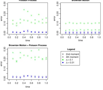
We have done a simple simulation to visualize the errors of the above toy example. For this we simulated 1000 sample paths of Brownian motion resp. of the Poisson process (with intensity 1) up to time 1 on a 0.0001 grid. Next we defined the approximations for

△ =

0

.

1 and 0.01 and calculated the empirical moments of the errors at times 0.0999, 0.1999,

. . .

. The result of the simulation can be seen inFig. 1. One difference between the theoretical discussion above and the actual simulation, is that the second and fourth empirical moments of the error in the Poisson case do usually coincide. This happens, since in a simulation one considers only finitely many paths and thus for

△

small enough, each of these paths has only at most one jump during a time step of size

△

. Therefore the error is zero or one and these are invariant under taking the second or fourth power.

Remark 3.2. As we stated in the Introduction section, there has been no systematic work so far on numerical schemes for SFDEs with jumps (pure jumps). As sequels to this work, we shall report two extensions in future work:

(i) Strong convergence ofEMnumerical schemes of SFDE with pure jumps

dx

(

t

)

=

f

(

xt

)

dt

+

h

(

xt−

)

dN

(

t

),

0

≤

t

≤

T

,

(3.15)

under condition

|

f

(ϕ)

−

f

(ψ )

|

2

_{∨ |}

_h

_(ϕ)

₋

_h

_{(ψ )}

_|

2

_≤

_L

_‖

_ϕ

₋

_ψ

_‖

2 _(3.16)

forL

>

0. Since all moments of the Poisson incrementsN

((

k

+

1

)

△

)

−

N

(

k

△

)

have the same order of

△

(

∈

(

0

,

1

))

, the challenge is to estimate

E



sup

1≤k≤M−1

‖¯

yk△

− ¯

y(k−1)△

‖

2



under condition(3.16), wherey

¯

k△is determined similarly by(2.7).

(ii) Invariant measure forEMnumerical solutions to Eq.(3.15). Based on the strong convergence established in problem (i), the key ingredient is to show the Markovian property ofy

¯

k△to show problem (ii).

4. Convergence rate under local Lipschitz condition

In this section, we shall discuss convergence rate ofEMnumerical solutions to(2.2)under the following local Lipschitz condition.

(H3) (Local Lipschitz condition) For each integerj

≥

1, there is a left-continuous nondecreasing function

µ

j

: [−

τ ,

0

] →

R+

such that

|

f

(ϕ)

−

f

(ψ )

|

2

_{∨ |}

_g

_(ϕ)

₋

_g

_{(ψ )}

_|

2

_{∨ |}

_h

_(ϕ)

₋

_h

_{(ψ )}

_|

2

_≤

∫

0

−τ

|

ϕ(θ )

−

ψ (θ )

|

2_d

_µ

j

(θ ),

(4.1)

for those

ϕ, ψ

∈ ˆ

Dwith

‖

ϕ

‖ ∨ ‖

ψ

‖ ≤

j.

(H4) (Linear growth condition) Assume that there is a constanth

>

0 such that for

ϕ

∈ ˆ

D

|

f

(ϕ)

|

2

∨ |

g

(ϕ)

|

2

∨ |

h

(ϕ)

|

2

≤

h

(

1

+ ‖

ϕ

‖

2

).

(4.2)

Remark 4.1. Under conditions(4.1)and(4.2), for any initial data

ξ

∈

Db

F

0

(

[−

τ ,

0

];

R

n

₎

_{,(2.2)admits a unique solution} x

(

t

),

t

∈ [

0

,

T

]

, by using the standard truncation procedure (see [3, Theorem 3.4, p56]). Moreover,(4.1)implies for those

ϕ, ψ

∈ ˆ

Dwith

‖

ϕ

‖ ∨ ‖

ψ

‖ ≤

j

|

f

(ϕ)

−

f

(ψ )

|

2

∨ |

g

(ϕ)

−

g

(ψ )

|

2

∨ |

h

(ϕ)

−

h

(ψ )

|

2

≤

Lj‖

ϕ

−

ψ

‖

2

,

(4.3)

[image:10.544.102.444.55.354.2]

Fig. 1. Simulation of the example—empirical errors.

Theorem 4.1. Let conditions(2.6),(4.1)and(4.2)hold. If there exist positive constants

α

and

ε

˜

∈

(

0

,

1

)

such that local Lipschitz constants obey

L1_j+˜ε

≤

α

logj

,

(4.4)

then

E



sup

0≤t≤T

|

x

(

t

)

−

y

(

t

)

|

2



=

O

(

△

2+2ϵ

_),

_(4.5)

where

ϵ

∈

(

0

,

ε)

˜

is an arbitrarily fixed small positive number.

Proof. Letj

≥

1 be an integer, and letSj

= {

x

∈

Rn

: |

x

| ≤

j

}

. Define the projection

π

j

:

Rn

→

Sjby

π

j

(

x

)

=

j

∧ |

x

|

|

x

|

x

,

where we set

π

j

(

0

)

=

0 as usual. It is easy to see that for allx

,

y

∈

Rn

|

π

j

(

x

)

−

π

j

(

y

)

| ≤ |

x

−

y

|

.

Define the operator

π

¯

j

: ˆ

D

→ ˆ

Dby

¯

π

j

(ϕ)

= {

π

j

(ϕ(θ ))

: −

τ

≤

θ

≤

0

}

.

Clearly,

‖ ¯

π

j

(ϕ)

‖ ≤

j

,

∀

ϕ

∈ ˆ

D

.

Define the truncation functionsfj

: ˆ

D

→

Rn,gj

: ˆ

D

→

Rn×mandhj

: ˆ

D

→

Rnby

respectively. Then, by(4.1), for any

ϕ, ψ

∈ ˆ

D

|

fj

(ϕ)

−

fj

(ψ )

|

2

∨ |

gj

(ϕ)

−

gj

(ψ )

|

2

∨ |

hj

(ϕ)

−

hj

(ψ )

|

2

≤ |

f

(

π

¯

j

(ϕ))

−

f

(

π

¯

j

(ψ ))

|

2

∨ |

g

(

π

¯

j

(ϕ))

−

g

(

π

¯

j

(ψ ))

|

2

∨ |

h

(

π

¯

j

(ϕ))

−

h

(

π

¯

j

(ψ ))

|

2

≤

∫

0

−τ

|

π

j

(ϕ(θ ))

−

π

j

(ψ (θ ))

|

2d

µ

j

(θ )

≤

∫

0

−τ

|

ϕ(θ )

−

ψ (θ )

|

2_d

_µ

j

(θ ).

(4.7)

That is,fj,gjandhjsatisfy the global Lipschitz condition. Fort

∈ [

0

,

T

]

, letxj

(

t

)

be the solution to the following SFDE with

jumps

dxj

(

t

)

=

fj

(

xjt

)

dt

+

gj

(

xjt

)

dB

(

t

)

+

hj

(

xj_t−

)

dN

(

t

)

with the initial dataxj₀

=

ξ

andyj

₍

_t

₎

_{be the corresponding continuous-timeEMsolution with the step size}

_△

_{. ByTheorem 3.1}

for any sufficiently small

ϵ

∈

(

0

,

ε)

˜

E



sup

0≤t≤T

|

xj

(

t

)

−

yj

(

t

)

|

2+ϵ



≤

δ

1L1

+ϵ/2 j e

δ2L1j+ϵ/2

_△

_.

Furthermore, by(4.4)(here we assumeLj

≥

1 without any loss of generality),

E



sup

0≤t≤T

|

xj

(

t

)

−

yj

(

t

)

|

2+ϵ



≤

e(δ1+δ2)Lj1+ϵ/2

_{△ ≤}

_jα(δ1+δ2)

_△

_.

_(4.8)

Set

ˆ

x

(

T

)

=

sup

0≤t≤T

|

x

(

t

)

|

and y

ˆ

(

T

)

=

sup

0≤t≤T

|

y

(

t

)

|

.

For any integerj

≥

1, define stopping time

τ

j

=

T

∧

inf

{

t

∈ [

0

,

T

] : ‖

xjt

‖ ∨ ‖

y j t

‖

>

j

}

.

It is easy to see that

‖

xjs‖ ≤jfor any 0

≤

s

< τ

j. Then, combining(4.6)gives that for any 0

≤

s

< τ

j

fj

(

xjs

)

=

f



‖

xjs

‖ ∧

j

‖

xjs‖ x j s



=

f



‖

xjs

‖ ∧

(

j

+

1

)

‖

xjs‖ x

j s



=

fj+1

(

xjs

)

=

f

(

x j s

).

Similarly,

gj

(

xjs

)

=

gj+1

(

xjs

)

=

g

(

x j

s

),

hj

(

xjs

)

=

hj+1

(

xjs

)

=

h

(

x j s

).

While on 0

≤

t

< τ

j

xj

(

t

)

=

ξ (

0

)

+

∫

t

0

fj

(

xjs

)

ds

+

∫

t

0

gj

(

xjs

)

dB

(

s

)

+

∫

t

0

hj

(

xj_s−

)

dN

(

s

)

=

ξ (

0

)

+

∫

t

0

fj+1

(

xjs

)

ds

+

∫

t

0

gj+1

(

xjs

)

dB

(

s

)

+

∫

t

0

hj+1

(

xj_s−

)

dN

(

s

)

=

ξ (

0

)

+

∫

t

0

f

(

xj_s

)

ds

+

∫

t

0

g

(

xj_s

)

dB

(

s

)

+

∫

t

0

h

(

xj

s−

)

dN

(

s

).

Consequently, we must have that

x

(

t

)

=

xj

(

t

)

=

xj+1

(

t

)

on 0

≤

t

< τ

j. Likewise, we can also derive that