Contents lists available atScienceDirect
Journal of Computational and Applied
Mathematics
journal homepage:www.elsevier.com/locate/cam
Convergence rate and stability of the truncated
Euler–Maruyama method for stochastic differential equations
Liangjian Hu
a, Xiaoyue Li
b,*
, Xuerong Mao
c aDepartment of Applied Mathematics, Donghua University, Shanghai 201620, ChinabCenter for Mathematics and Interdisciplinary Sciences, School of Mathematics and Statistics, Northeast Normal University, Changchun,
130024, China
cDepartment of Mathematics and Statistics, University of Strathclyde, Glasgow G1 1XH, UK
a r t i c l e i n f o
Article history:
Received 21 December 2016
Received in revised form 18 January 2018
Keywords:
Stochastic differential equation Khasminskii-type condition Truncated Euler–Maruyama method Convergence rate
Stability
a b s t r a c t
Recently, Mao (2015) developed a new explicit method, called the truncated Euler– Maruyama (EM) method, for the nonlinear SDE and established the strong convergence theory under the local Lipschitz condition plus the Khasminskii-type condition. In his another follow-up paper (Mao, 2016), he discussed the rates ofLq-convergence of the
truncated EM method forq ≥ 2 and showed that the order ofLq-convergence can
be arbitrarily close toq/2 under some additional conditions. However, there are some restrictions on the truncation functions and these restrictions sometimes might force the step size to be so small that the truncated EM method would be inapplicable. The key aim of this paper is to establish the convergence rate without these restrictions. The other aim is to study the stability of the truncated EM method. The advantages of our new results will be highlighted by the comparisons with the results in Mao (2015, 2016) as well as others on the tamed EM and implicit methods.
©2018 The Author(s). Published by Elsevier B.V. This is an open access article under the CC BY license (http://creativecommons.org/licenses/by/4.0/).
1. Introduction
Influenced by Higham, Mao and Stuart [1], the strong convergence theory of numerical methods for nonlinear stochastic differential equations (SDEs) without the global Lipschitz condition has become more and more popular. Although the classical Euler–Maruyama (EM) method is convenient for computations and implementations, the absolute moments of its approximation for SDEs with super-linear coefficients diverge to infinite at a finite time (see, e.g., [2]). Many implicit methods were used to study the numerical solutions to SDEs with nonlinear coefficients (see, e.g., [1,3–7]). Especially, Higham, Mao and Stuart [1] proved that the implicit EM numerical solutions converge strongly to the exact solutions of SDEs with globally one-sided Lipschitz continuous drift term and globally Lipschitz diffusion term, but the explicit EM method fails to do that. For the background on the implicit methods, we refer the reader to the books [8–10]. However, it is demonstrated that the implementation of the implicit EM method requires more computational effort. Recently, due to the advantages of explicit methods, Hutzenthaler, Jentzen and Kloeden proposed an explicit method for such SDEs called tamed Euler method whose numerical solutions converge strongly to the exact solution with 1
/
2 order. Sabanis in [11] went a further step to propose the modified tamed Euler method approximating the SDEs with superlinearly growing drift and diffusion coefficients, moreover, recovered the strong order 1/
2 in the estimation of convergence rate. Other explicit methods, such as the stopped EM method, as well as the tamed Milstein method, have been further developed (see, e.g., [12,13] for details).*
Corresponding author.E-mail addresses:[email protected](L. Hu),[email protected](X. Li),[email protected](X. Mao).
https://doi.org/10.1016/j.cam.2018.01.017
In particular, Mao [14] in 2015 proposed a new explicit method, called the truncated EM method. In his another follow-up paper [15], he investigated the convergence rates for the method under some additional conditions. We will point out that some of these additional conditions might force the step size to be so small that the truncated EM method would be inapplicable. One of our key aims in this paper is to establish the convergence rate without these restrictions so that the truncated EM method is more widely implementable. To overcome the difficulties due to removing these restrictions, some new mathematical techniques, which are significantly different from those used in [15], have been developed.
A nice numerical method should not only have an acceptable finite-time convergence rate but also have the ability to preserve the asymptotic properties of the underlying SDEs (see, e.g., [16,17]). Another aim of this paper is to show the ability of the truncated EM method to preserve the asymptotic stability of the underlying SDEs.
To show the advantages of the truncated EM method, we will compare it with other methods, e.g., the implicit EM method, the tamed Euler method and the modified tamed Euler method. We will design two numerical experiments and compute the errors between the true solution and the numerical solutions obtained by different schemes. It turns out that to achieve the same accuracy, the runtime of the truncated EM method and of the tamed Euler method are almost equivalent, but much shorter than that of the implicit EM method. However, to achieve the same accuracy, the step size for the modified tame Euler method is required to be smaller than that for the truncated EM method. These show clearly that the truncated EM method might be more efficient and is certainly suitable for the highly nonlinear SDEs.
The rest of the paper is organized as follows. Section2gives some notation and preliminary results on the numerical solution of the truncated EM method. Section3begins to demonstrate the improved convergence rate in a finite time interval. Section4goes further to compare our result with the previous convergence rate results. Section5makes use of the truncated EM method to approximate the asymptotic stability. Section6concludes our main results. TheAppendixproves that the classical EM method cannot reproduce asymptotic stability while the truncated method does.
2. Notation and lemmas
Throughout this paper, unless otherwise specified, we let (Ω
,
F,
P) be a complete probability space with a filtration{F
t}
t≥0satisfying the usual conditions (that is, it is right continuous and increasing whileF0contains allP-null sets), andletEdenote the probability expectation with respect toP. LetB(t) be anm-dimensional Brownian motion defined on the probability space and isFt-adapted. IfAis a vector or matrix, its transpose is denoted byAT. Ifx
∈
Rd, then|
x|
is theEuclidean norm. IfAis a matrix, we let
|
A| =
√
trace(ATA) be its trace norm. Moreover, for two real numbersaandb, we use a∨
b=
max(a,
b) anda∧
b=
min(a,
b). For a setG, its indicator function is denoted byIG, namelyIG(x)=
1 ifx∈
Gand 0 otherwise.Consider ad-dimensional nonlinear SDE
dx(t)
=
f(x(t))dt+
g(x(t))dB(t),
t≥
0,
(2.1)with the initial valuex(0)
=
x0∈
Rd, wheref:
Rd→
Rdandg:
Rd→
Rd×mare Borel measurable. We impose two standinghypotheses in this paper.
Assumption 2.1. Assume that the coefficientsfandgsatisfy the local Lipschitz condition: For anyR
>
0, there is aKR>
0 such that|
f(x)−
f(y)| ∨ |
g(x)−
g(y)| ≤
KR|
x−
y|
(2.2)for allx
,
y∈
Rdwith|
x| ∨ |
y| ≤
R.Assumption 2.2. Assume that the coefficients satisfy the Khasminskii-type condition: There is a pair of constantsp
>
2 andK
>
0 such thatxTf(x)
+
p−
1 2|
g(x)|
2
≤
K(1+ |
x|
2) (2.3)for allx
∈
Rd.We state a known result (see, e.g., [18,19]) as a lemma for the use of this paper.
Lemma 2.3. UnderAssumptions2.1and2.2, the SDE(2.1)has a unique global solution x(t)and, moreover,
sup 0≤t≤TE
|
x(t)|
p<
∞
,
∀
T>
0.
(2.4)Recall the truncated EM numerical scheme defined in [14]. We first choose a strictly increasing continuous function
µ
:
R+→
R+such thatµ
(u)→ ∞
asu→ ∞
andsup
|x|≤u
(
Denote by
µ
−1the inverse function ofµ
and we see thatµ
−1is a strictly increasing continuous function from[
µ
(1),
∞
) toR+. We also choose a constanth
ˆ
≥
1∨
µ
(1) and a strictly decreasing functionh:
(0,
1] → [
µ
(1),
∞
) such thatlim ∆→0h(∆)
= ∞
and ∆1/4h(∆)≤ ˆ
h,
∀
∆∈
(0,
1]
.
(2.6)We will see later thatAssumption 3.2implies(3.4), namely that both coefficientsfandggrow at most polynomially, whence we can let
µ
(u)=
H3u1+0.5ρ, whereH3is a positive constant specified in(3.4). Moreover, we can leth(∆)= ˆ
h∆−εfor someε
∈
(0,
1/
4]
. In other words, there are lots of choices forµ
(·
) andh(·
). Before we proceed, let us make a useful remark.Remark 2.4.In Mao [14] where the truncated EM was originally developed, it was required to choose a number∆∗
∈
(0
,
1]
and a strictly decreasing functionh:
(0,
∆∗] → [
µ
(0)
,
∞
) such thath(∆∗)
≥
µ
(2),
lim ∆→0h(∆)= ∞
and ∆1/4h(∆)≤
1,
∀
∆∈
(0,
∆∗]
.
Here, we simply let∆∗
=
1 and remove conditionh(∆∗)≥
µ
(2) while we also replace condition∆1/4h(∆)≤
1 by a weaker one∆1/4h(∆)≤ ˆ
h. In other words, we have made the choice of functionhmore flexible. We emphasize that such changes do not make any effect on the results in Mao [14,15]. In fact, conditionh(∆∗)
≥
µ
(2) was only used to prove [14, Lemma 2.4]. But, in view ofLemma 2.5, we see that the constant 2Kin [14, Lemma 2.4] is now replaced by another constantKˆ
which does not affect any other results in [14]. It is also easy to check that replacing∆1/4h(∆)≤
1 by∆1/4h(∆)≤ ˆ
hdoes not make any effect on the other results in [14]. Similarly, we see that these changes do not affect any results in [15] either.For a given step size∆
∈
(0,
1]
, let us define the truncated mappingπ
∆:
Rd→ {
x∈
Rd
: |
x| ≤
µ
−1(h(∆))}
byπ
∆(x)=
(
|
x| ∧
µ
−1(h(∆)))
x|
x|
,
where we setx
/
|
x| =
0 whenx=
0. That is,π
∆mapsxto itself if|
x| ≤
µ
−1(h(∆)) and toµ
−1(h(∆))x/
|
x|
if|
x|
> µ
−1(h(∆)). Define the truncated functionsf∆(x)
=
f(π
∆(x)) and g∆(x)=
g(π
∆(x)) (2.7)forx
∈
Rd. It is easy to see that|
f∆(x)| ∨ |
g∆(x)| ≤
µ
(µ
−1(h(∆)))=
h(∆),
∀
x∈
Rd.
(2.8)The discrete-time truncated EM numerical solutionsX∆(tk)
≈
x(tk) fortk=
k∆are formed by settingX∆(0)=
x0and computingX∆(tk+1)
=
X∆(tk)+
f∆(X∆(tk))∆+
g∆(X∆(tk))∆Bk,
(2.9)fork
=
0,
1, . . .
, where∆Bk=
B(tk+1)−
B(tk). There are two versions of the continuous-time truncated EM solutions. The first one is defined by¯
x∆(t)=
∞
∑
k=0
X∆(tk)I[tk,tk+1)(t)
,
t≥
0.
(2.10)This is a simple step process so its sample paths are not continuous. We will refer to it as the continuous-time step-process truncated EM solution. The other one is defined by
x∆(t)
=
x0+
∫
t0
f∆(x
¯
∆(s))ds+
∫
t0
g∆(x
¯
∆(s))dB(s) (2.11)fort
≥
0. We will refer to it as the continuous-time continuous-sample truncated EM solution. We observe thatx∆(tk)=
¯
x∆(tk)
=
X∆(tk) for allk≥
0. Moreover,x∆(t) is an Itô process with its Itô differentialdx∆(t)
=
f∆(x¯
∆(t))dt+
g∆(x¯
∆(t))dB(t).
(2.12)The following lemma shows that the truncated functionsf∆andg∆preserveAssumption 2.2very well.
Lemma 2.5. LetAssumption2.2hold. Then, for all∆
∈
(0,
1]
, we havexTf∆(x)
+
p−
1 2|
g∆(x)|
2
≤ ˆ
K(1+ |
x|
2),
∀
x∈
Rd
,
(2.13)whereK
ˆ
=
2K(
Proof. This lemma was essentially proved in [14] but we here do not need conditionh(∆∗
)
≥
µ
(2) as we already pointed out inRemark 2.4.Fix any∆
∈
(0,
1]
. Forx∈
Rdwith|
x| ≤
µ
−1(h(∆)), the required assertion(2.13)holds clearly. Forx∈
Rdwith
|
x|
> µ
−1(h(∆)), the proof of [14, Lemma 2.4] shows thatxTf∆(x)
+
p−
1 2|
g∆(x)|
2
≤
|
x|
µ
−1(h(∆))K(1+ [
µ
−1(h(∆))
]
2).
Noting that
µ
−1(h(∆))≥
µ
−1(h(1)), we then derivexTf∆(x)
+
p−
1 2|
g∆(x)|
2
≤
K|
x|
(
1µ
−1(h(1))+ |
x|
)
≤
K(
1∨ [
1/µ
−1(h(1))]
)
(|
x| + |
x|
2)≤
0.
5Kˆ
(1+
2|
x|
2)≤ ˆ
K(1+ |
x|
2)as required. □
RecallingRemark 2.4, we can then cite two lemmas from [14] on the continuous-time truncated EM solutions defined by (2.10)and(2.11)for the use of this paper.
Lemma 2.6. For any∆
∈
(0,
1]
and anypˆ
>
0, we haveE
|
x∆(t)− ¯
x∆(t)|
pˆ≤
cp∆ˆ ˆp/2(h(∆))pˆ
,
∀
t≥
0,
(2.14)where cpˆis a positive constant dependent only onp. Consequently
ˆ
lim ∆→0E
|
x∆(t)− ¯
x∆(t)|
ˆp=
0,
∀
t≥
0.
(2.15)Lemma 2.7. LetAssumptions2.1and2.2hold. Then
sup 0<∆≤1
(
sup 0≤t≤TE|
x∆(t)|
p)
≤
C,
∀
T>
0,
(2.16)where, and from now on, C stands for generic positive real constants dependent on T
,
p,
K,
x0,etc. but independent of∆and itsvalues may change between occurrences.
3. Convergence rates
Mao [14] established the theory ofLq-convergence for 2
≤
q<
pfor the truncated EM method, wherepis a parameter inAssumption 2.2. However, the convergence was in the asymptotic form without the convergence rate. Recently, Mao [15] investigated the convergence rates for the method under some additional conditions. However, there are some restrictions on the functionsµ
(·
) andh(·
) and these restrictions sometimes force the step size to be so small that the truncated EM method is inapplicable. We are now going to establish the convergence rates without these restrictions. We need some additional conditions.Assumption 3.1. Assume that there is a pair of constantsq
>
2 andH1>
0 such that(x
−
y)T(f(x)−
f(y))+
q−
12
|
g(x)−
g(y)|
2≤
H1
|
x−
y|
2 (3.1)for allx
,
y∈
Rd.Assumption 3.2. Assume that there is a pair of positive constants
ρ
andH2such that|
f(x)−
f(y)|
2∨ |
g(x)−
g(y)|
2≤
H2(1+ |
x|
ρ+ |
y|
ρ)|
x−
y|
2 (3.2)for allx
,
y∈
Rd.It is useful to observe that the truncated functionsf∆andg∆preserveAssumption 3.2perfectly. In fact, we derive that
|
f∆(x)−
f∆(y)|
2∨ |
g∆(x)−
g∆(y)|
2= |
f(π
∆(x))−
f(π
∆(y))|
2∨ |
g(π
∆(x))−
g(π
∆(y))|
2≤
H2(1+ |
π
∆(x)|
ρ+ |
π
∆(y)|
ρ)|
π
∆(x)−
π
∆(y)|
2for allx
,
y∈
Rd. Notingwe get
|
f∆(x)−
f∆(y)|
2∨ |
g∆(x)−
g∆(y)|
2≤
H2(1+ |
x|
ρ+ |
y|
ρ)|
x−
y|
2.
(3.3)Moreover, we also observe fromAssumption 3.2that
|
f(x)| ∨ |
g(x)| ≤
H3|
x|
(2+ρ)/2
,
∀|
x| ≥
1,
(3.4)whereH3
=
√
2H2
+ |
f(0)| + |
g(0)|
.To point out the restrictive condition imposed in [15], we cite its main result on the convergence rate.
Theorem 3.3([15]). LetAssumptions2.1,2.2,3.1and3.2hold with p
>
q and2p>
qρ
. Letq¯
∈ [
2,
q)(we have q>
2in Assumption3.1). Ifh(∆)
≥
µ
(
[
∆q¯/2(h(∆))¯q]
−1/(p−¯q))
(3.5)
for all sufficiently small∆
∈
(0,
1]
, then, for every such small∆,E
|
x(T)−
x∆(T)|
¯q≤
C∆q¯/2(h(∆))q¯ and E|
x(T)− ¯
x∆(T)|
q¯≤
C∆q¯/2(h(∆))q¯.
(3.6)In particular, if we choose h(u)
=
∆−εforε
∈
(0,
0.
25]
, it then follows from(3.6)thatE
|
x(T)−
x∆(T)|
¯q=
O(∆q¯(1−2ε)/2) and E|
x(T)− ¯
x∆(T)|
q¯=
O(∆q¯(1−2ε)/2).
(3.7)This theorem shows that the truncated EM method has the order ofL¯q-convergence close toq
¯
/
2. This is almost optimal in theory if we recall that the classical EM method has orderq¯
/
2 ofLq¯-convergence. However, condition(3.5)could sometimesmake the truncated EM method impracticable. For example, consider the case wherep
=
6,q¯
=
2,µ
(u)=
100u4/3andh(u)
=
u−0.25. Then(3.5)becomes∆≤
10−24. In other words, the step size is required to be extremely small. The key aim of this paper is to remove condition(3.5)and still to be able to establish the theory of the strong convergence rates. To overcome the difficulties without imposing condition(3.5), we develop some new mathematical techniques, which are significantly different from those used in [15], and get the following result on theLq¯-convergence rate. From now on, we will fixT>
0 arbitrarily.Theorem 3.4.LetAssumptions2.1,2.2,3.1and3.2hold and assume that2p
>
(2+
ρ
)q. Then, for anyq¯
∈ [
2,
q)and∆∈
(0,
1]
,E
|
x(T)−
x∆(T)|
¯q≤
C(
(
µ
−1(h(∆)))−(2p−(2+ρ)q¯)/2+
∆q¯/2(h(∆))¯q)
(3.8)
and
E
|
x(T)− ¯
x∆(T)|
¯q≤
C(
(
µ
−1(h(∆)))−(2p−(2+ρ)q¯)/2+
∆q¯/2(h(∆))¯q)
.
(3.9)In particular, recalling(3.4), we may define
µ
(u)=
H3u(2+ρ)/2
,
u≥
1,
(3.10)and let
h(∆)
=
∆−ε for someε
∈
(0,
1/
4]
andhˆ
≥
1, (3.11)to get
E
|
x(T)−
x∆(T)|
¯q=
O(
∆[ε(2p−(2+ρ)q¯)/(2+ρ)]∧[¯q(1−2ε)/2])
(3.12)and
E
|
x(T)− ¯
x∆(T)|
¯q=
O(
∆[ε(2p−(2+ρ)q¯)/(2+ρ)]∧[¯q(1−2ε)/2])
.
(3.13)Proof. Fixq
¯
∈ [
2,
q) and∆∈
(0,
1]
arbitrarily. Lete∆(t)=
x(t)−
x∆(t) fort≥
0. For each integern>
|
x0|
, define the stopping timeθ
n=
inf{
t≥
0: |
x(t)| ∨ |
x∆(t)| ≥
n}
,
where we set inf
∅ = ∞
(as usual∅
denotes the empty set). By the Itô formula, we have that for any 0≤
t≤
T,E
|
e∆(t∧
θ
n)|
q¯≤
E∫
t∧θn0
¯
q
|
e∆(s)|
q¯−2(
eT∆(s)
[
f(x(s))−
f∆(x¯
∆(s))] +
q¯
−
12
|
g(x(s))−
g∆(x¯
∆(s))|
Noting
¯
q−
12
|
g(x(s))−
g∆(¯
x∆(s))|
2≤
q¯
−
1 2[(
1
+
q− ¯
q¯
q−
1)
|
g(x(s))−
g(x∆(s))|
2+
(
1
+
q¯
−
1 q− ¯
q)
|
g(x∆(s))−
g∆(x¯
∆(s))|
2]
=
q−
12
|
g(x(s))−
g(x∆(s))|
2
+
(q¯
−
1)(q−
1)2(q
− ¯
q)|
g(x∆(s))−
g(¯
x∆(s))|
2,
we get from(3.14)that
E
|
e∆(t∧
θ
n)|
¯
q
≤
J1
+
J2,
(3.15)where
J1
=
E∫
t∧θn0
¯
q
|
e∆(s)|
q¯−2(
eT∆(s)
[
f(x(s))−
f(x∆(s))] +
q−
12
|
g(x(s))−
g(x∆(s))|
2
)
ds (3.16)and
J2
=
E∫
t∧θn0
¯
q
|
e∆(s)|
q¯−2(
eT∆(s)
[
f(x∆(s))−
f∆(x¯
∆(s))] +
(q¯
−
1)(q−
1)2(q
− ¯
q)|
g(x∆(s))−
g∆(x¯
∆(s))|
2
)
ds.
(3.17)ByAssumption 3.1, we have
J1
≤ ¯
qH1E∫
t∧θn0
|
e∆(s)|
q¯ds.
(3.18)RearrangingJ2, we get
J2
≤
E∫
t∧θn0
¯
q
|
e∆(s)|
¯q−2(
eT∆(s)
[
f(x∆(s))−
f∆(x∆(s))]
+
(q¯
−
1)(q−
1)(q
− ¯
q)|
g(x∆(s))−
g∆(x∆(s))|
2)
ds+
E∫
t∧θn0
¯
q
|
e∆(s)|
¯q−2(
eT∆(s)
[
f∆(x∆(s))−
f∆(x¯
∆(s))]
+
(q¯
−
1)(q−
1)(q
− ¯
q)|
g∆(x∆(s))−
g∆(¯
x∆(s))|
2)
ds=:
J21+
J22.
(3.19)We estimateJ21first. By the Young inequalityaq¯−2b
≤
(q¯
−
2)aq¯/
q¯
+
2bq¯/2/
q¯
for anya,
b≥
0 and 0≤
t∧
θ
n≤
t≤
T, we can show thatJ21
≤
E∫
t∧θn0
¯
q
|
e∆(s)|
¯q−2(
0
.
5|
e∆(s)|
2+
0.
5|
f(x∆(s))−
f∆(x∆(s))|
2+
(q¯
−
1)(q−
1)(q
− ¯
q)|
g(x∆(s))−
g∆(x∆(s))|
2)
ds≤
(q¯
−
1) 2(q−
2)(q
− ¯
q) E∫
t∧θn0
|
e∆(s)|
q¯ds+
E∫
t∧θn0
|
f(x∆(s))−
f∆(x∆(s))|
q¯ds+
2(q¯
−
1)(q−
1) (q− ¯
q) E∫
t∧θn0
|
g(x∆(s))−
g∆(x∆(s))|
q¯ds≤
C1E∫
t∧θn0
|
e∆(s)|
q¯ds+
J23,
(3.20)where
J23
=
C1E∫
t∧θn0
(
|
f(x∆(s))−
f∆(x∆(s))|
q¯+ |
g(x∆(s))−
g∆(x∆(s))|
q¯)
ds
and
C1
=
max{
(q
¯
−
1)2(q−
2) (q− ¯
q),
1,
2(q
¯
−
1)(q−
1) (q− ¯
q)}
Due tot
∧
θ
n≤
TandAssumption 3.2, we derive thatJ23
≤
C1E∫
T0
(
|
f(x∆(s))−
f(π
∆(x∆(s)))|
q¯+ |
g(x∆(s))−
g(π
∆(x∆(s)))|
¯q)
ds
≤
2×
3q¯/2H2C1∫
T0
E
(
(1
+ |
x∆(s)|
ρ¯q/2+ |
π
∆(x∆(s))|
ρ¯q/2)|
x∆(s)−
π
∆(x∆(s))|
¯q)
ds
≤
4×
3q¯/2H2C1∫
T0
E
(
(1
+ |
x∆(s)|
ρ¯q/2)|
x∆(s)−
π
∆(x∆(s))|
q¯)
ds
.
Using the Hölder inequality andLemma 2.7yields
J23
≤
4×
3¯
q/2H 2C1
∫
T0
(
E(1
+ |
x∆(s)|
p))
ρ2qp¯(
E
|
x∆(s)−
π
∆(x∆(s))|
2pq¯2p−ρq¯
)
2p2−pρ¯q ds≤
4×
3q¯/2H2C1(C+
1)ρ¯q 2p
∫
T 0(
E[
I{|x∆(s)|>µ−1(h(∆))}
|
x∆(s)|
2pq¯
2p−ρq¯
])
2p−ρ¯
q 2p
ds
≤
4×
3q¯/2H2C1(C+
1)ρ¯q 2p
∫
T0
([
P
{|
x∆(s)|
> µ
−1(h(∆))}
]
2p−(2+ρ)¯q 2p−ρ¯q
[
E
|
x∆(s)|
p]
2¯
q 2p−ρq¯
)
2p−ρq¯
2p ds
≤
4×
3q¯/2H2C1(C+
1)¯
q(ρ+2) 2p
∫
T0
(
E|
x∆(s)|
p(
µ
−1(h(∆)))p)
2p−(2+ρ)q¯
2p ds
≤
4×
3q¯/2H2C1(C+
1) (µ
−1(h(∆)))−2p−(2+ρ)q¯
2
.
Substituting this into(3.20)gives
J21
≤
C1E∫
t∧θn0
|
e∆(s)|
q¯ds+
4×
3¯q/2C1(C+
1) (µ
−1(h(∆)))− 2p−(2+ρ)¯q2
.
(3.21)Similarly, we can show
J22
≤
C3E∫
t∧θn0
|
e∆(s)|
q¯ds+
C4E∫
T0
(
E
|
x∆(s)− ¯
x∆(s)|
2p¯q/(2p−ρ¯q))
(2p−ρ¯q)/2pds
,
(3.22)whereC3,C4and the followingC5, etc. are generic constants independent of∆. ByLemma 2.6, we then have
J22
≤
C2E∫
t∧θn0
|
e∆(s)|
q¯ds+
C5∆¯
q/2(h(∆))q¯
.
(3.23)Combining(3.15),(3.18),(3.19),(3.21)and(3.23)together, we get
E
|
e∆(t∧
θ
n)|
q¯≤
C6(
E
∫
t∧θn0
|
e∆(s)|
q¯ds+
(µ
−1(h(∆)))−(2p−(2+ρ)¯q)/2+
∆q¯/2(h(∆))¯q)
≤
C6(
∫
t0
E
|
e∆(s∧
θ
n)|
q¯ds+
(µ
−1(h(∆)))−(2p−(2+ρ)q¯)/2+
∆¯q/2(h(∆))q¯)
.
(3.24)An application of the Gronwall inequality yields that
E
|
e∆(T∧
θ
n)|
q¯≤
C7(
(
µ
−1(h(∆)))−(2p−(2+ρ)¯q)/2+
∆q¯/2(h(∆))¯q)
.
Using the well-known Fatou lemma, we can letn
→ ∞
to obtain the desired assertion(3.8). The other assertion(3.9)follows from(3.8)andLemma 2.6. Finally, whenµ
is defined by(3.10), thenµ
−1(u)=
(u/
H3)2/(2+ρ). Substituting this and(3.11)into (3.8)we get
E
|
x(T)−
x∆(T)|
¯q≤
C(
∆ε(2p−(2+ρ)q¯)/(2+ρ)
+
∆¯q(1−2ε)/2)
,
which is the required assertion(3.12). Similarly, we can show(3.13). The proof is therefore complete. □
The following theorem shows that the order ofLq¯-convergence could be close toq
¯
/
2 arbitrarily.Theorem 3.5. LetAssumptions2.1,3.1and3.2hold and letAssumption2.2hold for any p
>
2. Letµ
(·
)and h(·
)be defined by(3.10)and(3.11). Then, for anyq
¯
∈ [
2,
q)and anyε
∈
(0,
1/
4),and
E
|
x(T)− ¯
x∆(T)|
q¯≤
O(
∆q¯(1−2ε)/2)
.
(3.26)Proof. Choosingpsufficiently large for
ε
(2p−
(2+
ρ
)q¯
)/
(2+
ρ
)>
q¯
(1−
2ε
)/
2,
we can get the assertions from(3.12)and(3.13)easily. □
This theorem shows that the order ofLq¯-convergence can be close toq
¯
/
2 arbitrarily. This is almost optimal if we recall that the classical EM method has orderq¯
/
2 ofLq¯-convergence under the global Lipschitz condition. Let us discuss an example toillustrate our theory before we make some comparisons to highlight the advantages of our new results on the convergence rates.
Example 3.6. Consider the scalar stochastic Ginzburgh–Landau equation (see, e.g., [8,20,21])
dx(t)
=
(ax(t)−
bx3(t))dt+
cx(t)dB(t),
(3.27)withx(0)
=
x0, whereB(t) is a scalar Brownian motion anda,
b,
care three positive numbers. Clearly, its coefficientsf(x)
=
ax−
bx3andg(x)=
cxare locally Lipschitz continuous forx∈
R, namely, satisfyAssumption 2.1. Also, for any p
>
2, we havexf(x)
+
p−
1 2|
g(x)|
2
=
ax2−
bx4+
(p−
1)c 22 x 2
≤
116b(2a
+
(p−
1)c2)2
.
That is,Assumption 2.2is satisfied for anyp
>
2. Moreover, for anyq>
2,(x
−
y)(f(x)−
f(y))+
q−
12
|
g(x)−
g(y)|
2≤
(
a
+
0.
5c2(q−
1))
(x−
y)2,
∀
x,
y∈
R.
This means thatAssumption 3.1is satisfied for anyq
>
2 withH1=
a+
0.
5c2(q−
1). Furthermore, we can show|
f(x)−
f(y)|
2∨ |
g(x)−
g(y)|
2≤
H2(1+ |
x|
4+ |
y|
4)|
x−
y|
2,
whereH2
=
2a2+
9b2+
c2. So,Assumption 3.2is also satisfied withρ
=
4. To applyTheorem 3.4, we still need to design functionsµ
andh. Noting thatsup
|x|≤u
(
|
f(x)| ∨ |
g(x)|
)≤
α
u3,
∀
u≥
1,
where
α
=
a+
b+
c, we can haveµ
(u)=
α
u3and its inverse functionµ
−1(u)=
(u/α
)1/3foru≥
α
. Forε
∈
(0,
1/
4]
, we defineh(∆)=
α
(1+ |
x0|
3)∆−εfor∆>
0. Now, for anyq¯
≥
2, we can choosepsufficiently large forε
(2p−
(2+
ρ
)q¯
)/
(2+
ρ
)>
q¯
(1−
2ε
)/
2.
We can therefore conclude byTheorem 3.5that the truncated EM solutions of the SDE(3.27)satisfy
E
|
x(T)−
x∆(T)|
q¯=
O(∆q¯(1−2ε)/2) and E|
x(T)− ¯
x∆(T)|
q¯=
O(∆q¯(1−2ε)/2).
That is, the order ofL¯q-convergence can be arbitrarily close toq
¯
/
2.Let us now compare the simulations by the implicit EM method, the tamed Euler Method and the truncated EM method. For this purpose, we setT
=
a=
b=
c=
1 andx(0)=
2. The SDE(3.27)thus reads asdx(t)
=
(x(t)−
x3(t))dt+
x(t)dB(t),
x(0)=
2 (3.28)fort
∈ [
0,
1]
.
Let∆=
1/
N,
tk=
∆k,
∆Bk=
B(tk+1)−
B(tk).In order to compute the approximation errors for the different schemes, we will make use of the explicit solutionx(t) of SDE(3.28). Taking the Bernoulli transformationu(t)
=
1/
x2(t) yieldsdu(t)
=
(u(t)+
2)dt−
2u(t)dB(t),
u(0)=
1/
4,
which is a linear SDE and its solution has a closed form. Thus, by solving the above SDE we get the explicit solution
x(t)
=
1[
1 4e−t−B(t)
+
2∫
t 0es−t+B(s)−B(t)ds
]
2.
To approximate the mean square error, for example, of the implicit EM method, we runM
=
1000 independent trajectories[
x(T)]
(i)and[ ˜
Y∆N
]
(i):(E
|
x(T)− ˜
YN∆|
2)1/2
≈
(
1
M M
∑
i=1
|[
x(T)]
(i)− [ ˜
YN∆]
(i)|
2)
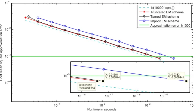
1/2Fig. 1. The root mean square approximation errors between the exact solutionx(T) of the SDE(3.28)and the numerical solutions:Y˜N∆by the implicit
EM scheme;Y˘N∆by the tamed Euler scheme;XN∆by the truncated EM scheme withε = 1/4, respectively, as functions of the runtime when∆ ∈ {2−7,2−8, . . . ,2−17}.
whereMdenotes the number of running independent trajectories.Fig. 1depicts the root mean square approximation errors between the exact solutionx(T) of the SDE(3.28)and the numerical solutions:Y
˜
N∆by the implicit EM scheme;Y˘
N∆by the tamed Euler scheme;XN∆by the truncated EM scheme withε
=
1/
4, respectively, as functions of the runtime when ∆∈ {
2−7,
2−8, . . . ,
2−17}
. When∆=
2−17, the runtime ofY˜
∆N,Y
˘
N∆andXN∆achieving the accuracy 0.000844 on our computer running at Intel Core i3-4170 CPU 3.70 GHz, is about 0.0383 s, 0.01901 s and 0.01812 s, respectively. In this case the runtime of the truncated EM method is the shortest.The Matlabcodes of simulating the implicit EM approximation and the tamed Euler approximation are from [21]. Our Matlabcodes for simulating the truncated EM approximationXN∆for SDE(3.28)are:
clear all
;
Y =2; Delta =2^( -17); N =2^17; v =9* Delta ^( -1/12);
for
n =1: N
if abs
(Y) >=v
Y=Y +( v*Y/
abs
(Y) -(v*Y/
abs
(Y ))^3)* Delta +...
(v*Y/
abs
(Y ))*
randn
*
sqrt
( Delta );
else
Y=Y +(Y -Y ^3)* Delta +Y*
randn
*
sqrt
( Delta );
end
end
4. Comparisons with known results
First of all, let us make a comparison between our newTheorem 3.4and one of the main results in [15], namely Theorem 3.3, in order to highlight the significant contribution of our new result. Although the assumptions imposed in both theorems are almost the same, we observe the following key differences:
•
The key feature ofTheorem 3.4is that it does not require the restrictive condition(3.5).•
The assertions ofTheorem 3.4hold for any∆∈
(0,
1]
while the assertions ofTheorem 3.3hold only for sufficiently small∆which satisfies condition(3.5).•
Theorem 3.4needs a slightly stronger condition on the parameters, namely 2p>
(2+
ρ
)q, which implies thatp>
qand 2p
>
qρ
imposed inTheorem 3.3.•
The assertions ofTheorem 3.4look slightly worse than those ofTheorem 3.3but could be the same whenpis large as demonstrated inTheorem 3.5.Example 4.1. Consider the scalar SDE
dx(t)
= −
10x3(t)dt+
x2(t)dB(t),
(4.1)whereB(t) is a scalar Brownian motion. Its coefficientsf(x)
= −
10x3andg(x)=
x2are clearly locally Lipschitz continuous forx∈
R. Forp=
21, we havexf(x)
+
p−
1 2|
g(x)|
2
=
0soAssumption 2.2is satisfied withp
=
21. Moreover, forq=
3, we have(x
−
y)(f(x)−
f(y))+
q−
12
|
g(x)−
g(y)|
2= −
10(x2+
xy+
y2)|
x−
y|
2+
(x+
y)2|
x−
y|
2= −
(9x2+
8xy+
9y2)|
x−
y|
2≤
0.
ThusAssumption 3.1holds withq
=
3. Furthermore, it is easy to show that|
f(x)−
f(y)|
2∨ |
g(x)−
g(y)|
2≤
800(1+
x4+
y4)|
x−
y|
2.
That is,Assumption 3.2is satisfied with
ρ
=
4.We first applyTheorem 3.3to see what we can get. Obviously, we havep
>
qand 2p>
qρ
and we chooseq¯
=
2. Noting|
f(x)| ∨ |
g(x)| ≤
10|
x|
3,
∀|
x| ≥
1,
we can then choose
µ
(u)=
10u3andh(∆)=
∆−1/4to define the truncated EM solutionx∆(t) to the SDE(4.1). It is easy to see that condition(3.5)becomes
∆−1/4
≥
10∆−3/38,
i.e., ∆≤
10−76/13=
1.
425103×
10−6.
For such a small step size,Theorem 3.3showsE
|
x(T)−
x∆(T)|
2∨
E|
x(T)− ¯
x∆(T)|
2≤
C∆0.5.
(4.2)The key issue here is that step size is required to be very small, namely less than 1
.
425103×
10−6, due to condition(3.5). Let us now apply our newTheorem 3.4to see if we can get a better result. Clearly, 2p>
(2+
ρ
)q. We letq¯
=
2,µ
(u)=
10u3 andh(∆)=
∆−1/4as before. Noting thatµ
−1(u)=
(u/
10)1/3and(
µ
−1(h(∆)))−(2p−(2+ρ)q¯)/2+
∆¯q/2(h(∆))q¯=
105∆5/4+
∆1/2=
O(∆0.5),
we conclude byTheorem 3.4that for any∆
∈
(0,
1]
,E
|
x(T)−
x∆(T)|
2∨
E|
x(T)− ¯
x∆(T)|
2≤
C∆0.5.
(4.3)This is the same as(4.2)but the step size∆can now be any number in (0
,
1]
rather than∆≤
1.
425103×
10−6.The advantage of our newTheorem 3.4is even more clear if we chooseh(∆)
=
∆−1/8while still useµ
(u)=
10u3to define the truncated EM solutionx∆(t). Letq¯
=
2 as before. In this case, condition(3.5)becomes∆−1/8
≥
10∆−9/76,
namely∆≤
1.
425103×
10−154.
This is almost impossible soTheorem 3.3is inapplicable. However, our newTheorem 3.4can still be applied. In fact, noting
(
µ
−1(h(∆)))−(2p−(2+ρ)q¯)/2+
∆¯q/2(h(∆))q¯=
105∆5/8+
∆6/8=
O(∆5/8),
we can then conclude, byTheorem 3.4, that for any∆
∈
(0,
1]
,E
|
x(T)−
x∆(T)|
2∨
E|
x(T)− ¯
x∆(T)|
2≤
C∆5/8,
(4.4)where
µ
(u)=
10u3andh(∆)=
∆−1/8are used to define the truncated EM solutionx∆(t) to the SDE(4.1). In other words, our newTheorem 3.4is not only applicable in this situation but also shows that the truncated EM solutionx∆(t) defined by using
µ
(u)=
10u3andh(∆)=
∆−1/8has a better strong convergence rate to the true solution of the SDE(4.1)than that usingµ
(u)=
10u3andh(∆)=
∆−1/4.Let us now compare the truncated EM method with the modified tamed Euler scheme (see, e.g., [11]) numerically. Consider the SDE(4.1)withx(0)
=
1 andT=
1. Since there is no explicit solution, we use the modified tamed Euler solution (see, e.g., [11]) with∆=
2−17as a good approximation of the exact solution.Fig. 2depicts the root mean square approximation error (E|
x(T)− ¯
YN∆|
2
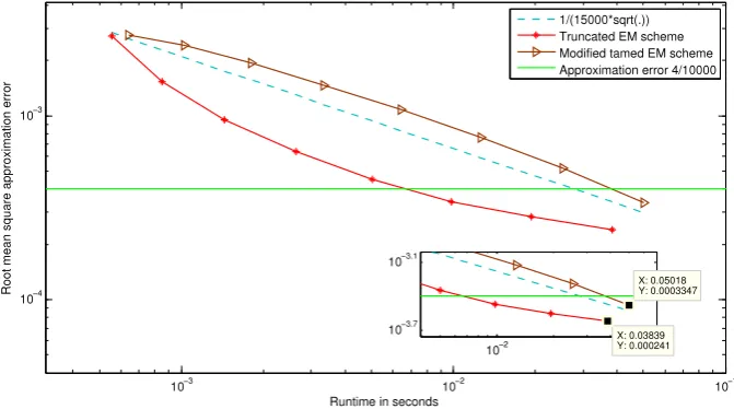
Fig. 2. The root mean square approximation errors between the exact solutionx(T) of the SDE(3.28)and the numerical solutions:Y¯∆
N by the modified
tamed Euler scheme;XN∆by the truncated EM scheme, respectively, as functions of runtime for∆∈ {2−7,2−8, . . . ,2−14}.
Fig. 3. The root mean square approximation errors between the exact solutionx(T) of the SDE(3.28)and the numerical solutions:Y¯∆
N by the modified
tamed Euler scheme,XN∆by the truncated EM scheme, respectively, as functions of runtime forT∈ {1,2, . . . ,10}with the same step size∆=2
−14.
ofY
¯
N∆achieving the accuracy 0.0003347 on our computer with Intel Core i3-4170 CPU 3.70 GHz, is about 0.05018 s while the runtime ofXN∆achieving the accuracy 0.000241 is about 0.03839 s (see the enlargement inFig. 2). Thus, the speed of the truncated Euler scheme for the SDE(4.1)is 1.3 times faster than that of the modified tamed Euler scheme, while the accuracy achieved by the truncated Euler scheme is almost 1.4 times better than that of the modified tamed Euler scheme. Moreover, for step size∆=
2−14, we go further to simulate the root mean square approximation error for different values of timeT. Fig. 3depicts the root mean square approximation error(
E
⏐
⏐
x(T)− ¯
Y2−14 N
⏐
⏐
2
)
1/2between the exact solution of the SDE(3.28)
and the numerical solution by the modified tamed Euler scheme, and the error
(
E⏐
⏐
x(T)−
X2−14 N
⏐
⏐
2
)
1/2between the exact solution and that of the truncated EM scheme with
ε
=
1/
4,M=
1000, as functions of running time, forT∈ {
1,
2, . . . ,
10}
.The Matlabcodes for simulating the modified tamed Euler approximationY
¯
k∆are:clear all
;
Y =1; Delta =2^( -14); N =2^14; alpha =0.5; l =2;
for
n =1: N
Y=Y +1/(1+ n^( - alpha )*
abs
(Y )^ l )*( -10* Y ^3)* Delta +...
1/(1+ n^( - alpha )*
abs
(Y )^ l )* Y ^2*
randn
*
sqrt
( Delta );
[image:11.544.105.440.282.473.2]5. Asymptotic stability
In this section we will discuss if the truncated EM method can preserve the asymptotic stability of the underlying SDE (2.1). We will let the assumptions imposed in the previous sections as the standing hypotheses so we will not mention them explicitly in the theorem in this section. Moreover, for the stability purpose (see, e.g., [18]), we also assume in this section that
f(0)
=
0,
g(0)=
0.
(5.1)We need an additional assumption to guarantee the asymptotic stability of the underlying SDE(2.1). We need one more notation. LetKdenote the family of continuous non-decreasing functions
κ
:
R+→
R+such thatκ
(0)=
0 andκ
(u)>
0for allu
>
0.Assumption 5.1. Assume that there is a function
κ
∈
Ksuch that2xTf(x)
+ |
g(x)|
2≤ −
κ
(|
x|
) (5.2)for allx
∈
Rd.Let us state a theorem which follows easily from [22].
Theorem 5.2. LetAssumption5.1hold. Then for any initial value x0
∈
Rd, the solution of the SDE(2.1)satisfieslim
t→∞x(t)
=
0 a.
s.
(5.3)The following theorem shows that the truncated EM method can preserve this almost surely asymptotical stability with an additional condition(5.4). We will see from the example below that this additional condition is not restrictive.
Theorem 5.3. LetAssumption5.1hold. Assume also that
lim sup
|x|↓0
|
f(x)|
2κ
(|
x|
)<
∞
.
(5.4)Set
H
=
sup0<|x|≤µ−1(h(1))
|
f(x)|
2κ
(|
x|
) (5.5)and
ˆ
∆=
min(
1
,
0.
5/
H,
0.
25(κ
(µ
−1(h(1)))/
hˆ
)2)
.
(5.6)Then for every∆
∈
(0,
∆ˆ
]
and any initial value x0∈
Rd, the solution of the truncated EM method(2.9)satisfieslim k→∞X∆(tk)
=
0 a.
s.
(5.7)Proof. We first observe thatH
<
∞
from condition(5.4)and the continuity off(·
) as well as the property ofκ
(·
) and hence we have∆ˆ
∈
(0,
1]
.We next show that the truncated functionsf∆andg∆preserve property(5.2)perfectly in the sense that, for any∆
∈
(0,
1]
,2xTf∆(x)
+ |
g∆(x)|
2≤ −
κ
(|
π
∆(x)|
),
x∈
Rd.
(5.8)In fact, this holds obviously forx
∈
Rdwith|
x| ≤
µ
−1(h(∆)). Forx∈
Rdwith
|
x|
> µ
−1(h(∆)), we derive, byAssumption 5.1,2xTf∆(x)
+ |
g∆(x)|
2=
2(x−
π
∆(x))Tf(π
∆(x))+
2(π
∆(x))Tf(π
∆(x))+ |
g(π
∆(x))|
2≤
2(x−
π
∆(x))Tf(π
∆(x))−
κ
(|
π
∆(x)|
).
(5.9)But, byAssumption 5.1again,
2(x
−
π
∆(x))Tf(π
∆(x))=
2[|
x|
/µ
−1(h(∆))−
1]
(π
∆(x))Tf(π
∆(x))≤
0.
Let us now fix any∆
∈
(0,
∆ˆ
]
andx0∈
Rd. It is easy to derive from(2.9)and(5.8)that|
X∆(tk+1)|
2=
|
X∆(tk)|
2+
2X∆(tk)Tf∆(X∆(tk))∆+ |
g∆(X∆(tk))|
2∆+ |
f∆(X∆(tk))|
2∆2+
∆Mk≤
|
X∆(tk)|
2−
κ
(|
π
∆(X∆(tk))|
)∆+ |
f∆(X∆(tk))|
2∆2+
∆Mk (5.10)fork
=
0,
1, . . .
, where∆Mk
=
2(X∆(tk)+
f∆(X∆(tk))∆)Tg∆(X∆(tk))∆Bk+ |
g∆(X∆(tk))∆Bk|
2− |
g∆(X∆(tk))|
2∆.
(5.11)Note
E
(
|
g∆(X∆(tk))∆Bk|
2⏐
⏐F
tk)
=
E(
trace[
g∆(X∆(tk))∆Bk∆BTkg∆(X∆(tk))T]⏐
⏐F
tk)
=
trace[
g∆(X∆(tk))E(
∆Bk∆BTk⏐
⏐F
tk)
g∆(X∆(tk))T]
=
trace[
g∆(X∆(tk))∆Img∆(X∆(tk))T]
=
∆|
g∆(X∆(tk))|
2,
whereImdenotes them
×
midentity matrix. It is then easy to show thatE(∆Mk
|F
tk)=
0.
This implies immediately that
Mk
:=
k∑
i=0
∆Mi
,
k=
0,
1,
2, . . . ,
(5.12)is a martingale. Using(5.5)and recalling that
µ
−1(h(∆))≥
µ
−1(h(1)), we hence have|
f∆(x)|
2= |
f(x)|
2≤
Hκ
(|
x|
)=
Hκ
(|
π
∆(x)|
) if 0≤ |
x| ≤
µ
−1(h(1)).
On the other hand, if
|
x|
> µ
−1(h(1)), we have|
f∆(x)|
2≤
(h(∆))2≤
(h(∆)) 2κ
(µ
−1(h(1)))κ
(|
π
∆(x)|
).
Consequently, for allx∈
Rd,|
f∆(x)|
2∆≤
κ
(|
π
∆(x)|
) max{
H∆
,
(h(∆))2∆
κ
(µ
−1(h(1)))}
≤
κ
(|
π
∆(x)|
) max{
H∆
,
ˆ
h2√
∆κ
(µ
−1(h(1)))}
≤
0.
5κ
(|
π
∆(x)|
),
where(2.6)and(5.6)have been used. Substituting this into(5.10), we get
|
X∆(tk+1)|
2≤ |
X∆(tk)|
2−
0.
5κ
(|
π
∆(X∆(tk))|
)∆+
∆Mk,
k≥
0.
(5.13)This implies
|
X∆(tk+1)|
2≤ |
x0|
2−
0.
5∆ k∑
i=0
κ
(|
π
∆(X∆(ti))|
)+
Mk,
k≥
0.
(5.14)Applying the nonnegative semi-martingale convergence theorem (see, e.g., [23, Theorem 7 on page 139] or [9, Theorem 1.10 on page 18]), we get
∞
∑
i=0
κ
(|
π
∆(X∆(ti))|
)<
∞
a.
s.
This implies
lim i→∞
κ
(|
π
∆(X∆(ti))|
)=
0 a.
s.
Consequently, we must have
lim
i→∞
![Fig. 4. (a) Sample paths of the classical EM solution ln|Y(t)|; (b) Sample paths of the truncated EM solution x∆(t) with the same initial value x0 = 10 fordifferent values of step size ∆ and t ∈ [0, 90].](https://thumb-us.123doks.com/thumbv2/123dok_us/1386391.91815/14.544.103.440.55.192/sample-classical-solution-sample-truncated-solution-initial-fordifferent.webp)
